This is a repository copy of
Dealing with Massive Data with a Distributed Expectation
Propagation Particle Filter for Object Tracking
.
White Rose Research Online URL for this paper:
http://eprints.whiterose.ac.uk/100348/
Version: Accepted Version
Proceedings Paper:
De Freitas, A. and Mihaylova, L.S. orcid.org/0000-0001-5856-2223 (2016) Dealing with
Massive Data with a Distributed Expectation Propagation Particle Filter for Object
Tracking. In: Information Fusion (FUSION), 2016 19th International Conference on. 19th
International Conference on Information Fusion, 04-08 Jul 2016, Heidelberg, Germany.
IEEE . ISBN 978-0-9964-5274-8
© 2016 IEEE. Personal use of this material is permitted. Permission from IEEE must be
obtained for all other users, including reprinting/ republishing this material for advertising or
promotional purposes, creating new collective works for resale or redistribution to servers
or lists, or reuse of any copyrighted components of this work in other works.
[email protected] https://eprints.whiterose.ac.uk/
Reuse
Unless indicated otherwise, fulltext items are protected by copyright with all rights reserved. The copyright exception in section 29 of the Copyright, Designs and Patents Act 1988 allows the making of a single copy solely for the purpose of non-commercial research or private study within the limits of fair dealing. The publisher or other rights-holder may allow further reproduction and re-use of this version - refer to the White Rose Research Online record for this item. Where records identify the publisher as the copyright holder, users can verify any specific terms of use on the publisher’s website.
Takedown
If you consider content in White Rose Research Online to be in breach of UK law, please notify us by
Dealing with Massive Data with a Distributed
Expectation Propagation Particle Filter for Object
Tracking
Allan De Freitas, Lyudmila Mihaylova
Department of Automatic Control and Systems Engineering, University of Sheffield, United Kingdom Emails:[email protected], [email protected]
Abstract—Target tracking in distributed networks faces the challenge in coping with large volumes of distributed data which requires efficient methods for real time applications with minimal communication overhead. The complexity considered in this paper is when each sensor in a distributed network observes a large number of measurements which are all required to be processed at each time step. The particle filter has been widely used for localisation and tracking in distributed networks with a small number of measurements [1]. This paper goes beyond the current state-of-the-art and presents a novel particle filter ap-proach, combined with the expectation propagation framework, that is capable of dealing with the challenges presented by a large volume of measurements in a distributed network. In the proposed algorithm, the measurements are processed in parallel at each sensor node in the network and the communication overhead is minimised substantially. We show results with large improvements in communication overhead, with a negligible loss in tracking performance, compared with the standard centralised particle filter.
I. INTRODUCTION
In large scale surveillance systems, varying numbers and different types of electronic sensors are typically used to track objects. Examples of such systems include freeway traffic monitoring systems [2] and wireless sensor networks [3]. However, recent technological advances have lead to the availability of cheap, high resolution sensors. This can result in a massive amount of measurements being collected by each sensor. In a tracking application it is required to process the data online to obtain estimates of the objects. In a Bayesian framework, this involves the sequential inference of the filtering distribution associated with a state space model. This can be a challenging task when dealing with a large number of measurements.
An additional challenge is when the state space model is characterised by non-linearities and/or non-Gaussian noises. In such scenarios, a closed form solution for the filtering distribu-tion is typically not available. Sequential Monte Carlo (SMC) methods [4], or particle filters (PFs), are a popular set of techniques which are used to obtain a discrete approximation for the filtering distribution. The PF has been successfully ap-plied to a wide variety of areas. However, PFs are susceptible to weight degeneracy and sample impoverishment [5] under certain conditions, as well as potentially high computational times.
In this paper we consider an interconnected network of sensor nodes. The measurements observed by a single sensor may be insufficient to accurately estimate the states which describe objects in the surrounding environment, due to model complexities. Thus, the sensor nodes are required to cooper-atively estimate the states. The measurements can either be processed locally at each sensor node, or globally, by first communicating all of the measurements to a central processing node. In the latter case, a single PF can be utilised to obtain an estimate. In [6] the measurements were quantised prior to transmission to a central processing node. However, in the context of a large amount of measurements, this can still incur an intolerable communication cost.
In static Markov chain Monte Carlo (MCMC) simulation, there have been several different approaches proposed for dealing with large amounts of data [16]. Techniques based on divide and conquer focus on subdividing the measurements and running separate MCMC samplers in parallel on each subdivided set of measurements. The samples from the sepa-rate MCMC samplers, referred to as local samples, are then combined to obtain samples from the complete posterior distri-bution, referred to as global samples. The divide and conquer techniques differ in how the local samples are combined to obtain the global samples. In [17], global samples are obtained as a weighted average of the local samples. This approach is only theoretically valid under a Gaussian assumption. In [18], the local posterior from the separate MCMC samplers is approximated as Gaussian or with a Gaussian kernel density estimation. Global samples can then be obtained through the product of the local densities. This idea is also further developed in [19] by representing the discrete kernel density estimation as a continuous Weierstrass transform. In [20], the combination is based on the geometric median of the local pos-teriors which are approximated with Weiszfeld’s algorithm by embedding the local posteriors in a reproducing kernel Hilbert space. Divide and conquer techniques typically face difficulties in applications where the local posteriors substantially differ, and if they do not satisfy Gaussian assumptions. In [21], [22] a divide and conquer strategy was proposed which attempts to overcome the challenge of differing local posteriors, and relaxing the Gaussian assumption to a more general assump-tion of a posterior distribuassump-tion from the exponential family. The approach is based on the expectation propagation (EP) algorithm.
The two challenges associated with distributed target track-ing with large volumes of data are: computational complexity due to the processing of the data and significant communi-cation costs when required to transmit large volumes of data across a network. In this paper we propose a novel method, based on the combination of the PF and the EP framework, which overcomes these challenges for object tracking in an interconnected network of sensor nodes. The method is well suited to handling a large number of measurements from each sensor node. This includes a large number of measurements which are not generated by the object being tracked, referred to as clutter measurements.
The remainder of this paper is organised in the following manner: Section II gives details of the proposed estimation method. This includes the introduction of the centralised PF in Section II-A, and the EP-PF in Section II-B. Section III describes the experiments performed and the performance met-rics used. Section IV illustrates the performance improvements of the EP-PF in comparison with the centralised PF. Finally, conclusions are summarised in Section V.
II. PROBLEMFORMULATION
We consider a sensor network consisting of D sensor nodes. Each sensor node d generates a set of measurements at each time tk, with k = 1, ..., T ∈N, represented by a set
zd,k ={z1d,k, ...,z Md,k
d,k }, where Md,k is the total number of
measurements from sensor node d, and zid,k ∈ R nz
. Object tracking in a sensor network can be considered as a sequen-tial state estimation problem within a Bayesian framework. The aim is to sequentially compute the filtering posterior distribution p(xk|z1:k), where xk ∈ Rnx
is the state vector representing the hidden states of the objects at time tk, and
z1:k ={z1, ...,zk}, represents all the measurements received
up till timetk, where zj=S D
d=1zj,d. The filtering posterior
distribution can be recursively updated through a two step process when the the filtering posterior distribution at the previous time step, p(xk−1|z1:k−1), is available. The first
step is referred to as the prediction step via the Chapman-Kolmogorov equation, resulting in the predictive posterior distribution [4].
p(xk|z1:k−1) = Z
p(xk|xk−1)p(xk−1|z1:k−1)dxk−1, (1)
where p(xk|xk−1) represents the state transition probability
density function (pdf), which relates the hidden state at the previous time step to the hidden state at the current time step. The new measurements are utilised to update the predictive posterior distribution via Bayes’ rule
p(xk|z1:k) =
p(xk|z1:k−1)p(zk|xk)
R
p(xk|z1:k−1)p(zk|xk)dxk
, (2)
where p(zk|xk) is referred to as the likelihood probability
density function, which relates the measurements to the hidden states at the current time step. An analytical solution to equa-tions (1) and (2) is typically intractable when the state space model is characterised by non-linearities and/or non-Gaussian noise. The PF is an SMC technique capable of computing an approximation of the filtering posterior distribution under such conditions [23], [24].
A. Centralised Particle Filter
We introduce the theory of the generic PF by describing the centralised PF (CPF) which forms the primary basis of comparison with the novel technique presented in Section II-B. In the CPF, the measurements from all D sensor nodes are transmitted to a central processing node at each time step. The PF consists of a discrete set ofN samples, commonly referred to as particles, with corresponding weights {x(kj), wk(j), j =
1, . . . , N}. The weighted particles approximate the filtering posterior distribution
b
p(xk|z1:k), N
X
j=1
w(kj)δ
xk−x
(j)
k
, (3)
whereδ(·)denotes the Dirac delta function, and the weights are normalised such that Pjw
(j)
k = 1. The particles and
each time step every particle is updated by sampling from an appropriate proposal distribution:
x(kj)∼q(xk|x( j)
k−1,zk). (4)
The particles weight corrects for the mismatch between the filtering posterior distribution and the proposal distribution. The unnormalised weight is updated according to:
wk(j)∝w
(j)
k−1
p(x(kj)|x
(j)
k−1)p(zk|x( j)
k )
q(x(kj)|xk(j−)1,zk)
. (5)
However, this procedure is equivalent to sampling from a state space whose dimension size is linked to the time step,k, due to sampling the entire path history of the state variables up to the current time step. This leads to weight degeneracy. In order to reduce this, the PF resamples the particles according to the weights. This allows for the favouring of highly weighted par-ticles while discarding less favourable parpar-ticles. Unfortunately this can lead to sample impoverishment, which is when there are a high number of duplicated particles. The lack of diversity in the particle set can result in filter degeneracy. To prevent sample impoverishment, it has been proposed to only perform sampling when weight degeneracy occurs. A commonly used measure for weight degeneracy is the effective sample size [24].
A detailed description of the generic CPF is described in Algorithm 1.
Algorithm 1 Centralised Particle Filter
1: Initialise particle set:{x(0j)}N
j=1 according to prior
distri-bution.
2: fork= 1,. . . ,T do
3: Transfer the measurements from each of the D sensor nodes to the central processing node.
4: forj = 1,. . . ,N do
5: Sample a particle:x(kj)∼q(xk|x( j)
k−1,zk).
6: Update the particle weight:
wk(j)=w
(j)
k−1
p(x(kj)|xk(j−)1)p(zk|x(kj)) q(x(kj)|xk(j−)1,zk)
7: end for
8: Normalise the weights:wk(j)= w(kj)
P iw
(i) k
j= 1, . . . , N. 9: ifResampling then
10: SelectN particle indices ji∈ {1, . . . , N} according
to weights{wk(j)} N j=1.
11: Setx(ki)=x(ji)
k , andw
(i)
k = 1/N i= 1, . . . , N.
12: end if 13: pb(xk|z1:k) =
PN
j=1w (j)
k δ
xk−x
(j)
k
14: end for
B. Expectation Propagation and the Particle Filter
When the measurements from the sensor nodes are consid-ered independent, it is possible to further reduce the global
filtering posterior distribution in (2) to the following represen-tation:
p(xk|z1:k)∝p(xk|z1:k−1)
D
Y
d=1
p(zk,d|xk). (6)
This results in the definition of a local likelihood for each sensor node d,p(zk,d|xk). The challenge lies in the fact that
each sensor node only has access to its own measurements. EP is a deterministic approximate inference scheme, based on the minimisation of the Kullback-Leibler (KL) divergence [25]. Typically the EP approach is used to approximate posterior distributions with a simpler distribution, which is close in the sense of the KL divergence. EP is a flexible scheme which naturally extends to distributed processing. In this paper, the EP framework is utilised to approximate the likelihood terms for each processing node with a member of the exponential family. This is done not due to the complexity of the likelihood terms, but rather to be able to represent them with a consistently small number of real numbers, thus minimising communications.
The local filtering posterior distribution at each processing nodedis given by:
pd(xk|z1:k)∝p(zk,d|xk)p(xk|z1:k−1) Y
i6=d
π(xk|ηi), (7)
with
π(xk|η) =h(x)g(η) exp
ηTu(x) , (8) where η represents the natural parameters (NPs), and h(x), g(η) and u(x) are functions which vary depending on the member of the exponential family. Clearly, the local filtering posterior distribution takes information about the measure-ments from the other processing nodes into account, thus being an approximation of the global posterior distribution, pd(xk|z1:k)≈p(xk|z1:k). The degree to which the
approxi-mation is true is dependent on how accurately the likelihood terms are approximated.
Given the natural parameters for the likelihood terms of all the neighbouring processing nodes, it is possible to obtain an approximation of the local filtering posterior distribution in (7). Due to the non-linearities and/or non-Gaussian noises in the state space model, a PF is utilised to obtain a discrete weighted approximation of the filtering posterior distribution,
b
pd(xk|z1:k), in the same form as in equation (3).
It is required to compute the natural parameters. Then the likelihood term for node d in (7) is replaced by the approximated likelihood term:
e
pd(xk|z1:k)∝π(xk|ηd)p(xk|z1:k−1) Y
i6=d
π(xk|ηi). (9)
The natural parameters can then be found through the minimi-sation of the KL divergence, KL(bpd(xk|z1:k)||ped(xk|z1:k)).
It has been shown [25] that this is equivalent to matching the moments,
E b
whereE[·]represents the mathematical expectation operation. By approximating the PF’s discrete approximation for the fil-tering posterior distribution with the same exponential family, π(xk|ηa,d) ≈ pbd(xk|z1:k), and similarly for the predictive
posterior distribution, π(xk|ηb,d) ≈ p(xk|z1:k−1), then the
natural parameter update is given by
ηd=ηa,d−ηb,d−
X
i6=d
ηi, (11)
whereηa,d andηb,d represent the respective natural
parame-ters. The processing nodes then share the natural parameters characterising the local likelihood with the other nodes in the network.
This procedure is generally iterated until reaching conver-gence. However, convergence is not always guaranteed. In this paper we treat the number of iterations as a fixed parameter, L.
A detailed description of the EP-PF is described in Algo-rithm 2.
Algorithm 2 Expectation Propagation Particle Filter: Algo-rithm for sensor noded.
1: Initialise particle set:{x(0j)}N
j=1 according to prior
distri-bution.
2: fork= 1,. . . ,T do
3: forℓ= 1,. . . ,Ldo
4: ifℓ == 1then
5: initialise the NPs from the set D\ d of sensor nodes:{ηi}i6=d.
6: end if
7: forj = 1,. . . ,N do
8: Sample a particle:x(kj)∼q(xk|x
(j)
k−1,zk).
9: Update the particle weight:
wk(j)=w
(j)
k−1
p(x(kj)|xk(j−)1)p(zk,d|xk)Qi6=dπ(xk|ηi)
q(x(kj)|xk(j−)1,zk)
.
10: end for
11: Normalise the weights:w(kj)= w(kj)
P iw
(i) k
j= 1, . . . , N. 12: ifResampling then
13: SelectN particle indicesji∈ {1, . . . , N}
accord-ing to weights{w(kj)} N j=1.
14: Setx(ki)=x(ji)
k , andw
(i)
k = 1/N i= 1, . . . , N.
15: end if
16: Estimate the following NPs: ηa,d and ηb,d, using
standard techniques (See Section III-B). 17: Compute the NPs for sensor noded:
ηd=ηa,d−ηb,d−
P
i6=dηi
18: Transmit the NPs for sensor nodedto the setD\d of sensor nodes.
19: Receive the NPs for the setD\dof sensor nodes . 20: end for
21: pbd(xk|z1:k) =P N j=1w
(j)
k δ
xk−x
(j)
k
22: end for
C. Particle Filter Proposal Distributions
Selecting the proposal distribution is an important step dur-ing the design of a PF. Utilisdur-ing a good proposal distribution results in the particles being moved to regions in the state space with higher likelihood values, which helps avoid weight degeneracy. It has been shown [26] that the optimal proposal distribution is the distribution which minimises the variance of the importance weights,
q(xk|x( j)
k−1,zk) =p(xk|x( j)
k−1,zk). (12)
However, sampling from this proposal distribution is generally not tractable. There are a variety of techniques which have been proposed to approximate the optimal proposal distribu-tion [4]. A common approach is to simply utilise the transidistribu-tion density,
q(xk|x( j)
k−1,zk) =p(xk|x( j)
k−1), (13)
due to its direct availability. This approach also simplifies the weight update to be proportional to the evaluation of the likelihood. However, the transition density does not include any information from the measurements and thus moves the particles blindly.
The EP-PF framework allows for an intuitive inclusion of information from the measurements at the neighbouring nodes in the proposal distribution. This can be done when the prior distribution is the same, or approximated as a member of the exponential family used to approximate the likelihood terms. The resulting proposal distribution is given by
q(xk|x
(j)
k−1,zk) =π(xk|ηp), (14)
where ηp = ηc +
P
i6=dηi, and ηc represents the natural
parameters of the transition density.
III. APPLICATION TO OBJECT TRACKING IN A COMPLEX SYSTEM
A. Target and Sensor Modelling
In this application the state vector consists of the posi-tion and velocity of a target in a two dimensional space, xk = [xk, yk,x˙k,y˙k]T. The target motion prediction is
performed according to the near constant velocity model [27]. This results in the state transition density having the form
p(xk|xk−1) =N(xk|Akxk−1,Qk), (15)
where N(·) represents the normal distribution, and matri-ces Ak and Qk are defined as Ak =
I2 TsI2
02 I2
and
Qk = σ2x
(T3
s/3)I2 (Ts2/2)I2
(T2
s/2)I2 TsI2
, whereTs=tk−tk−1.
In this application, the total number of measurements re-ceived at node d is given by Md,k = Md,kx +M
c
d,k, where
Mx
d,k represents the number of target measurements, andM c d,k
mean λX and λC respectively. The local likelihood density
thus takes the form [28]:
p(zd,k|xk)∝ MYd,k
i=1
λXpX(zid,k|xk) +λCpC(zid,k), (16)
where pX(·) and pC(·) represent the likelihood of the
tar-get and clutter measurements respectively. In the case of a measurement from the target, the likelihood is modelled as pX(zid,k|xk) = N(zd,ki ;h(xk),Σ), where h(xk) =
q
(xk−Sd,x)2+ (yk−Sd,y)2, and (Sd,x, Sd,y) T
represent the position coordinates of sensor node d. The clutter mea-surements are independent of the state of the target and are uniformly distributed in the visible region of the sen-sor, resulting in the clutter likelihood taking the form of pC(zid,k) =UR(zid,k).
B. Discussion
In this paper the multivariate Gaussian distribution is the member of the exponential family which is utilised to model the likelihood terms. In this case the NPs are given by
η= (Σ−1µ,Σ−1)T, (17)
where µ and Σ−1 represent the mean and precision of the
multivariate Gaussian distribution respectively. The sample mean and precision of the PF’s discrete approximations of pd(xk|z1:k)andp(xk|z1:k−1)are used to obtain the NPsηa,d
andηb,d, respectively.
It is important to note that the difference between two positive definite matrices in equation (11), may not be itself positive definite. Techniques, such as Sof tAbs [29], can be used to ensure that the result remains positive definite.
An important consideration is the communication cost of the different network topologies. Due to the many different variables associated with the speed of a communication link, we only consider the number of doubles which are required to be transmitted between nodes by each algorithm in order to infer the filtering posterior distribution. In the CPF, it is required to transmit all the measurements from each sensor node at each time step, to a centralised processing node. Assuming that each sensor node is capable of communicating with the processing node in parallel, then the number of doubles required to be transmitted is given by
CCPF= max
1≤d≤DMd,k. (18)
For an interconnected network, the communication cost of broadcasting the natural parameters of each sensor node in the EP-PF is related to the number of EP iterations,
CEP-PF= (L−1)NNP, (19) where NNP is the number of doubles used to represent the NPs.
IV. RESULTS
Consider the scenario of a target moving through a highly cluttered environment. A distributed sensor network, consist-ing of several sensor nodes, is utilised to monitor the target which returns multiple target and clutter measurements at each time step and each sensor node. Both the standard CPF, described in Algorithm 1, and the EP-PF, described in Algorithm 2, are utilised for the inference of the latent states of the target over several experiments with different parameters. Three different metrics are used to compare the performance of the filters. The first metric is the root mean square error (RMSE) of the position [27]. The RMSE for each time step is calculated over a number of independent simulation runs according to
RM SE=
v u u
t 1
NI NI
X
i=1
( ˆXi−Xi)2, (20)
whereX represents a specific component of the state vector xk, with Xi the ground truth, Xˆi represents the algorithm
estimate, which corresponds to the mean of the N MCMC samples in this application, and NI represents the number of
independent runs. The RMSE of the states corresponding to the position are averaged to obtain a single result. The RMSE of the position illustrates the tracking accuracy of the two algorithms.
The second metric is the effective sample size (ESS) [24], given by:
Nef f =
1
PN
j=1
wk(j)2
. (21)
The ESS illustrates the extent of weight degeneracy by giving an estimate of the number of informative particles in the PF.
Finally, we consider the communication cost for both tech-niques according to equation (18) and (19).
A. Parameters
The following parameters were utilised across all simu-lations, unless otherwise specified. The number of particles for the CPF and EP-PF are N = 10000, and N = 5000, respectively. The number of independent simulation runs is NI = 50. The number of time simulation steps is T = 70.
The motion model parameters areTs= 1, and σx= 0.5. The
number of sensor nodes isD= 4, respectivelyD= 8in the second experiment. The target observation model parameters areλX = 200andλX= 100 for the second experiment, and
Σ=I. The clutter parameters are: λC = 100 andλC = 50
for the second experiment, andAc= 4×10⁴. The number of
EP iterations is L= 2. B. Performance Evaluation
The target trajectory and sensor node positions relative to the target for the experiments are illustrated in Figure 1.
0 10 20 30 40 50 60 70 80 90 100
0 20 40 60 80 100
x (m)
y
(m
)
[image:7.612.59.295.51.253.2]Target Trajectory Starting Point End Point Sensor Node
Fig. 1: Object trajectory and sensor node placement for the experiments.
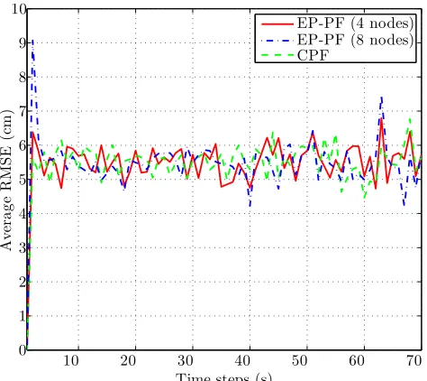
determines how many times the particle set is required to be re-evaluated. Results are illustrated for the minimum number of EP iterations. For the case of 4 sensor nodes, only the sensor nodes located in the corners in Figure 1 are considered. The overall number of measurements on average is the same for both 4 and 8 sensor nodes. The average RMSE for the position is illustrated in Figure 2. When considering more nodes in the
0 1 2 3 4 5 6 7 8 9 10
10 20 30 40 50 60 70
Time steps (s)
Av
er
a
g
e
R
M
S
E
(c
m
)
EP-PF (4 nodes) EP-PF (8 nodes) CPF
Fig. 2: Average RMSE for the position of the target.
EP-PF, the degree of approximation in equation (7) is greater, which results in a larger spike in the initial error. Overall, there is a negligible loss in tracking accuracy when using the EP-PF with only 2 EP iterations when compared to the CPF.
[image:7.612.359.517.82.128.2]For the given experimental setup, the communication cost
TABLE I: Average number of communicated doubles for one time cycle (fromk tok+ 1) for each approach.
Approach Average number of communicated doubles per
sensor node
CPF 300
[image:7.612.357.516.190.248.2]EP-PF 20
TABLE II: Normalised ESS averaged over all simulation runs. The value for the EP-PF is additionally averaged across allD sensor nodes.
Algorithm Normalised ESS
CPF 0.03
EP-PF (L= 1, D= 4) 0.24
EP-PF (L= 2, D= 4) 0.26
EP-PF (L= 1, D= 8) 0.32
EP-PF (L= 2, D= 8) 0.31
is given in Table I. It is clear from this result that a significant advantage of the EP-PF algorithm is the massive reduction in communication cost. This is due to the ability of the EP-PF to transmit the information found within the measurements at each sensor node in a fixed small number of NPs.
Finally the ESS, normalised by the number of particles, and averaged over all simulation runs is illustrated in Table II. During the first EP iteration the high ESS for the EP-PF can be explained by the fact that only a subset of the total measurements are evaluated at each node, resulting in a broad likelihood. In the second EP iteration the high ESS in the EP-PF is attributed to the improved proposal distribution which is described in Section II-C. This highlights the greater amount of information represented by the particles in the EP-PF.
V. CONCLUSIONS
In this paper we propose a novel method for object track-ing in a distributed network, referred to as the expectation propagation particle filter. The EP-PF has several advantages including: i) the EP-PF does not rely on a synchronous random number generator; ii) the EP-PF is scalable to any sized interconnected network of sensor nodes; iii) the EP-PF is capable of intuitively integrating measurement information in the proposal distribution; iv) the EP-PF framework allows for an approximation of the filtering distribution at every sensor node in the network; and v) the EP-PF is well suited to handle large volumes of measurements due to significantly reducing communication costs.
We present results illustrating that the EP-PF has up to a 93% reduction in the communication costs compared with a centralised PF framework.
ACKNOWLEDGMENTS
[image:7.612.58.295.412.623.2]2013-2017] TRAcking in compleX sensor systems (TRAX) Grant agreement no.: 607400.
REFERENCES
[1] O. Hlinka, F. Hlawatsch, and P. Djuric, “Distributed particle filtering in agent networks: A survey, classification, and comparison,”IEEE Signal Process. Mag., vol. 30, no. 1, pp. 61–81, Jan. 2013.
[2] L. Mihaylova, A. Hegyi, A. Gning, and R. Boel, “Parallelized Particle and Gaussian Sum Particle Filters for Large-Scale Freeway Traffic Systems,”IEEE Trans. on Intell. Transp. Syst., vol. 13, no. 1, pp. 36–48, March 2012.
[3] F. Zhao and L. J. Guibas,Wireless Sensor Networks: An Information Processing Approach. Amsterdam, The Netherlands: Morgan Kauf-mann, 2004.
[4] O. Cappe, S. Godsill, and E. Moulines, “An Overview of Existing Methods and Recent Advances in Sequential Monte Carlo,”Proc. IEEE, vol. 95, no. 5, pp. 899 –924, May 2007.
[5] T. Bengtsson, P. Bickel, and B. Li, Curse-of-dimensionality revisited: Collapse of the particle filter in very large scale systems, ser. Collections. Beachwood, Ohio, USA: Institute of Mathematical Statistics, 2008, vol. 2, pp. 316–334.
[6] Y. Ruan, P. Willett, A. Marrs, F. Palmieri, and S. Marano, “Practical fusion of quantized measurements via particle filtering,”IEEE Trans. Aerosp. Electron. Syst., vol. 44, pp. 15–29, Jan. 2008.
[7] X. Sheng and Y.-H. Hu, “Distributed particle filters for wireless sensor network target tracking,” inProc. IEEE Int. Conf. Acoustics, Speech, and Signal Processing., vol. 4, March 2005, pp. 845–848.
[8] Q. Cheng and P. Varshney, “Joint State Monitoring and Fault Detection using Distributed Particle Filtering,” inProc. Asilomar Conf. on Signals, Systems and Computers., Nov. 2007, pp. 715–719.
[9] D. Ustebay, M. Coates, and M. Rabbat, “Distributed auxiliary particle filters using selective gossip,” inProc. IEEE Int. Conf. Acoustics, Speech and Signal Processing., May 2011, pp. 3296–3299.
[10] C. Bordin and M. Bruno, “Consensus-based distributed particle filtering algorithms for cooperative blind equalization in receiver networks,” in Proc. IEEE Int. Conf. Acoustics, Speech and Signal Processing, May 2011, pp. 3968–3971.
[11] B. Oreshkin and M. Coates, “Asynchronous distributed particle filter via decentralized evaluation of Gaussian products,” inProc. 13th Int. Conf. on Information Fusion, July 2010, pp. 1–8.
[12] D. Gu, “Distributed EM Algorithm for Gaussian Mixtures in Sensor Networks,”IEEE Trans. Neural Netw., vol. 19, no. 7, pp. 1154–1166, July 2008.
[13] O. Hlinka, F. Hlawatsch, and P. Djuric, “Consensus-based Distributed Particle Filtering With Distributed Proposal Adaptation,”IEEE Trans. Signal Process., vol. 62, no. 12, pp. 3029–3041, June 2014.
[14] M. Coates, “Distributed particle filters for sensor networks,” inProc. IPSN, Berkeley, CA, April 2004, pp. 99–107.
[15] S. Dias and M. Bruno, “Cooperative Particle Filtering for Emitter Tracking with Unknown Noise Variance,” in Proc. IEEE Int. Conf. Acoustics, Speech and Signal Processing, March 2012, pp. 2629–2632. [16] R. Bardenet, A. Doucet, and C. Holmes, “Markov chain Monte Carlo
and tall data,”preprint, http://arxiv.org/abs/1505.02827, May 2015. [17] S. L. Scott, A. W. Blocker, F. V. Bonassi, H. A. Chipman, E. I. George,
and R. E. McCulloch, “Bayes and big data: The consensus Monte Carlo algorithm,” inEFaB Bayes 250 Conf., vol. 16, 2013.
[18] W. Neiswanger, C. Wang, and E. Xing, “Asymptotically Exact, Embar-rassingly Parallel MCMC,”preprint, http://arxiv.org/abs/1311.4780v2, 2013.
[19] X. Wang and D. Dunson, “Parallel MCMC via Weierstrass sampler,” preprint, http://arxiv.org/abs/1312.4605, 2014.
[20] S. Minsker, S. Srivastava, L. Lin, and D. Dunson, “Robust and Scal-able Bayes via a Median of Subset Posterior Measures,” preprint, http://arxiv.org/abs/1403.2660v2, 2014.
[21] M. Xu, Y. W. Teh, J. Zhu, and B. Zhang, “Distributed Context-Aware Bayesian Posterior Sampling via Expectation Propagation,” in Proc. Advances in Neural Information Processing Systems, 2014.
[22] A. Gelman, A. Vehtari, P. Jylnki, C. Robert, N. Chopin, and J. P. Cunningham, “Expectation propagation as a way of life,” preprint, http://arxiv.org/abs/1412.4869, 2014.
[23] A. Doucet, N. de Freitas, and N. Gordon, Eds.,Sequential Monte Carlo Methods in Practice. Spring-Verlag, 2001.
[24] M. Arulampalam, S. Maskell, N. Gordon, and T. Clapp, “A tutorial on particle filters for online nonlinear/non-Gaussian Bayesian tracking,” IEEE Trans. Signal Proc., vol. 50, no. 2, pp. 174 –188, Feb. 2002. [25] C. M. Bishop,Pattern Recognition and Machine Learning.
Springer-Verlag New York, 2006.
[26] A. Doucet, S. Godsill, and C. Andrieu, “On sequential Monte Carlo sampling methods for Bayesian filtering,” Statistics & Computing, vol. 10, no. 3, pp. 197–208, July 2000.
[27] Y. Bar-Shalom, X. R. Li, and T. Kirubarajan, Estimation with Appli-cations to Tracking and Navigation, 1st ed. Wiley-Interscience, June 2001.
[28] K. Gilholm and D. Salmond, “Spatial distribution model for tracking extended objects,”IEE Proc. Radar, Sonar and Navigation, vol. 152, no. 5, pp. 364–371, Oct. 2005.