Determination of a source in the heat equation from integral observations

promoting access to White Rose research papers

White Rose Research Online

Universities of Leeds, Sheffield and York

http://eprints.whiterose.ac.uk/

This is the Author's Accepted version of an article published in the Journal of Computational and Applied Mathematics

White Rose Research Online URL for this paper:

http://eprints.whiterose.ac.uk/id/eprint/78512

Published article:

Hào, DN, Thanh, PX, Lesnic, D and Ivanchov, M (2014) Determination of a source in the heat equation from integral observations. Journal of Computational and Applied Mathematics, 264. 82 - 98. ISSN 0377-0427

Determination of a source in the heat equation from integral

observations

Dinh Nho H`ao1,2, Phan Xuan Thanh3, D. Lesnic2, and M. Ivanchov4

1 _{Hanoi Institute of Mathematics, 18 Hoang Quoc Viet Road, Hanoi, Vietnam}

e-mail: [email protected]

2 _{Department of Applied Mathematics, University of Leeds, Leeds LS2 9JT, UK}

e-mail: [email protected]

3_{School of Applied Mathematics and Informatics,}

Hanoi University of Science and Technology, 1 Dai Co Viet Road, Hanoi, Vietnam

e-mail: [email protected]

4 _{Faculty of Mechanics and Mathematics, Ivan Franko National University of Lviv,}

1 Universytetska Str., Lviv, 79000 Ukraine

e-mail: [email protected]

November 5, 2013

Abstract

A novel inverse problem which consists of the simultaneous determination of a source together with the temperature in the heat equation from integral observations is investigated. These integral observations are weighted averages of the temperature over the space domain and over the time interval. The heat source is sought in the form of a sum of two space- and time-dependent unknown components in order to ensure uniqueness of solution. The local existence

and uniqueness of the solution in classical H¨older spaces are proved. The inverse problem is

linear, but it is ill-posed because small errors in the input integral observations cause large errors in the output source. For a stable reconstruction a variational least-squares method with or without penalization is employed. The gradient of the functional which is minimized is calculated explicitly and the conjugate gradient method is applied. Numerical results obtained for several benchmark test examples show accurate and stable numerical reconstructions of the heat source.

Keywords: Heat equation, heat source, conjugate gradient method, inverse problem.

1

Introduction

lack of uniqueness of solution in the general case when the source depends on both space and time, [10]. That is why inverse problems for finding sources depending on various/several variables are of great interest. For example, it is possible to restore uniqueness if we seek the source as a linear combination of point sources, [1], or as an additive, [11], or multiplicative, [20], expression of separate time and space-dependent continuous components.

The objective of this paper is to determine heat source functions depending on both space and time, but which are the sum of two unknown components depending separately on space and time, with known weights depending on time and space, respectively. The additional measure-ments/overspecified conditions are given by integral observations of the temperature over space and time. This is particular advantageous in practical applications where local point or instant temperature measurements contain too large errors and then the use of non-local average measure-ments appears more realistic and reliable.

The inverse problem is linear, but ill-posed. The local existence and uniqueness of a classical

solution in H¨older spaces are established in section 2, but more importantly this novel inverse

formulation based on non-local average integral observations rather than local space or time point measurement enables the development of a weak solution theory for which variational methods are at hand, as developed in section 3. The discretization of the direct and adjoint problems is based on the finite element method (FEM) which is briefly discussed in section 4. The iterative conjugate gradient method (CGM) employed for minimizing the least-squares gap between the measured and computed data is also presented in section 4. As expected, since the solution of the inverse problem does not depend continuously on the input data, regularization needs to be enforced in order to obtain a stable solution. This is performed by either stopping the CGM iteration at a threshold given by the discrepancy principle, or by penalizing the least-squares functional with extra regularization terms. Numerical results obtained for several benchmark test examples are presented and discussed in section 5. Finally, section 6 gives the conclusions of the paper.

2

Mathematical Formulation

In this paper, we consider the particular practical application of the inverse analysis in the search of the heat source distribution in a multi-dimensional conductor. The determination of this heat source distribution across the space and time solution domain has a significant importance on finding the characteristics and performances of the thermal field. Further, it also assists in the designing of new heat conducting devices with an improved performance.

Let Ω be a bounded domain in Rn with boundary ∂Ω, and T a given positive number. Denote

Q:= Ω×(0, T], andS :=∂Ω×(0, T]. In [11], the problem of determining the right hand coefficients

f1(x) andf2(t) in the Dirichlet problem

ut= ∆u+g0(x, t) +f1(x)g1(t) +f2(t)g2(x), (x, t)∈Q, (2.1)

u|t=0 =u0(x), x∈Ω, (2.2)

from the two additional conditions

u(x0, t) =h(t), t∈[0, T], (2.4)

∫ T

0

u(x, t)dt=g(x), x∈Ω,¯ (2.5)

where x0 is a fixed point in Ω, has been considered. Based on the trivial identity (f1(x) +

cg2(x))g1(t) + (f2(t) −cg1(t))g2(x) = f1(x)g1(t) +f2(t)g2(x), where c is an arbitrary constant,

one can see that problem (2.1)–(2.5) does not have a unique solution. However, if one imposes the

additional condition that f1(x0) is known then, under some conditions on the smoothness of the

data and their compatibility, it can be established, see [11], that if T is small, then there exists a

unique solution to the inverse problem. The aim of our paper is to solve this inverse source problem by a variational method. Since the pointwise measurement (2.4) cannot be defined in the usual weak form framework, we replace it by the integral measurement

l1u:=

∫

Ω

ω1(x)u(x, t)dx=h(t), t∈(0, T), (2.6)

whereω1 is a given function.

We also assume that we have available as prescribed the quantity ∫

Ω

ω1(x)f1(x)dx=C0. (2.7)

Then we have the following local uniqueness solvability theorem.

Theorem 2.1. Suppose that the following conditions are satisfied:

(A1) Equation (2.2) holds for x ∈ Ω, equation (2.3) holds on S and equation (2.6) holds for

t∈[0, T];

(A2) u0 ∈ H2+γ(Ω), g ∈ H2+γ(Ω), us ∈ H2+γ,1+γ/2(Ω), g0 ∈ Hγ(Ω), h ∈ H1+γ/2[0, T], ω1 ∈

H2+γ(Ω), ∂Ω∈H2+γ, where γ∈(0,1);

(A3) u0|∂Ω = us(·,0)|∂Ω, g|∂Ω =

∫T

0 us(·, t)|∂Ωdt, h(0) =

∫

Ωω1(x)u0(x)dx,

∫

Ωω1(x)g(x)dx =

∫T

0 h(t)dt;

(A4) ∫₀Tg1(t)dt̸= 0,

∫

Ωω1(x)g2(x)dx̸= 0, g1(t)/

∫T

0 g1(τ)dτ ≥0, t∈[0, T].

Then for sufficiently small T >0 there exists a unique solution (f1, f2, u)∈Hγ(Ω)×Hγ/2[0, T]×

H2+γ,1+γ/2(Q) of the inverse problem given by equations (2.1)–(2.3)and (2.5)–(2.7).

For the definition of the above H¨older spaces involved, see [14, p. 7].

Proof. Differentiating (2.6) yields

h′(t) =

∫

Ω

ω1(x)ut(x, t)dx=

∫

Ω

ω1(x)

(

∆u(x, t) +g0(x, t) +f1(x)g1(t) +f2(t)g2(x)

) dx

= ∫

Ω

(

u(x, t)∆ω1(x) +ω1(x)(g0(x, t) +f1(x)g1(t))

)

dx+f2(t)

∫

Ω

ω1(x)g2(x)dx

+ ∫

∂Ω

( ω1(x)

∂u

∂ν(x, t)−us(x, t)

∂ω1

∂ν (x, t)

Rearranging we obtain

f2(t) =

1 ∫

Ωω1(x)g2(x)dx

[ h′(t)−

∫

Ω

(ω1(x)g0(x, t) +u(x, t)∆ω1(x))dx−C0g1(t)

+ ∫

∂Ω

(us(x, t)

∂ω1

∂ν (x, t)−ω1(x)

∂u

∂ν(x, t))dS

]

, t∈[0, T]. (2.8)

Integrating (2.8) and using (2.5) we obtain ∫ T

0

f2(t)dt=

1 ∫

Ωω1(x)g2(x)dx

[

h(T)−h(0)−

∫ T

0

∫

Ω

ω1(x)g0(x, t)dxdt−

∫

Ω

g(x)∆ω1(x)dx

−C0

∫ T

0

g1(t)dt+

∫

∂Ω

(g(x)∂ω1

∂ν (x)−ω1(x)

∂g

∂ν(x))dS

]

= ∫ 1

Ωω1(x)g2(x)dx

[

h(T)−h(0)−

∫

Q

ω1(x)g0(x, t)dxdt

−

∫

Ω

ω1(x)∆g(x)dx−C0

∫ T

0

g1(t)dt

]

:=F1. (2.9)

We remark that F1 is known from the data of the problem.

Taking the Laplacian of (2.5) yields

∆g(x) = ∫ T

0

∆u(x, t)dt=

∫ T

0

(ut(x, t)−g0(x, t)−f1(x)g1(t)−f2(t)g2(x))dt

=u(x, T)−u0(x)−

∫ T

0

g0(x, t)dx−f1(x)

∫ T

0

g1(t)dt−g2(x)

∫ T

0

f2(t)dt.

Using (2.9) and rearranging we obtain

f1(x) =

1 ∫T

0 g1(t)dt

[

u(x, T)−u0(x)−

∫ T

0

g0(x, t)dx−∆g(x)−g2(x)F1

]

, x∈Ω. (2.10)

Let U0 ∈C2,1(Q)∩C1,0(Q) be the solution of the direct problem (2.1) with f1 = f2 = 0 subject

to (2.2) and (2.3). Then, ifGis the Green function of the Dirichlet problem for the heat equation

(2.1) withf1 =f2 =g0 = 0, the solutionu(x, t) possesses the representation

u(x, t) =U0(x, t) +

∫ t

0

∫

Ω

G(x, t;ξ, τ)

(

f1(ξ)g1(τ) +f2(τ)g2(ξ)

)

dξdτ, (x, t)∈Q. (2.11)

Applying (2.11) fort=T and substituting into (2.10) we obtain

f1(x) =f01(x) +

1 ∫T

0 g1(t)dt

∫ T

0

∫

Ω

G(x, T;ξ, τ) (

f1(ξ)g1(τ) +f2(τ)g2(ξ)

)

dξdτ, x∈Ω, (2.12)

where

f01(x) =

1 ∫T

0 g1(t)dt

[

U0(x, T)−u0(x)−

∫ T

0

g0(x, t)dx−∆g(x)−F1g2(x)

]

= ∫_T 1

0 g1(t)dt

[ ∫ T

0

∆U0(x, t)dt−∆g(x)−F1g2(x)

]

is a known function from the data of the problem. Also, taking the gradient of (2.11) multiplied

with the outward unit normalν and substituting into (2.8) we obtain

f2(t) =

1 ∫

Ωω1(x)g2(x)dx

{

h′(t)−C0g1(t)−

∫

Ω

ω1(x)g0(x, t)dx+

∫

∂Ω

us(x, t)

∂ω1

∂ν (x)dS

−

∫

∂Ω

ω1(x)

[_∂U

0

∂ν (x, t) +

∫ t 0 ∫ Ω ∂G ∂νx

(x, t;ξ, τ)(f1(ξ)g1(τ) +f2(τ)g2(ξ)

) dξdτ ] dSx − ∫ Ω

∆ω1(x)

[

U0(x, t) +

∫ t

0

∫

Ω

G(x, t;ξ, τ)(f1(ξ)g1(τ) +f2(τ)g2(ξ))dξdτ

] dx

} ,

or

f2(t) =f02(t)−

1 ∫

Ωω1(x)g2(x)dx

∫ t 0 ∫ Ω ( ∫ Ω

ω1(x)∆xG(x, t;ξ, τ)dx

)

×(f1(ξ)g1(τ) +f2(τ)g2(ξ))dξdτ, t∈[0, T], (2.14)

where

f02(t) =

1 ∫

Ωω1(x)g2(x)dx

[

h′(t)−C0g1(t)−

∫

Ω

ω1(x)g0(x, t)dx+

∫

∂Ω

us(x, t)

∂ω1

∂ν (x)dS

−

∫

∂Ω

ω1(x)

∂U0

∂ν (x, t)dS−

∫

Ω

∆ω1(x)U0(x, t)dx

]

= ∫ 1

Ωω1(x)g2(x)dx

[

h′(t)−C0g1(t)−

∫

Ω

ω1(x)

∂U0

∂t (x, t)dx

]

, t∈[0, T] (2.15)

is a known function from the data of the problem. Now the problem is equivalent to the coupled system of equations formed with the Fredholm integral equation (2.12) and the Volterra integral

equation (2.14), and the functionsf01(x) andf02(t) are known from the data of the problem. It is

shown in [11] that the equation

f1(x) =f01(x) +

1 ∫T

0 g1(t)dt

∫ T

0

∫

Ω

G(x, T;ξ, τ)f1(ξ)g1(τ)dξdτ, x∈Ω,

has a unique solution which may be represented in terms of the resolvent Γ(x, ξ). So, the function

f1(x) can be expressed via the functionf2(t) in the following way:

f1(x) =

∫

Ω

Γ(x, y) (

f01(y) +

1 ∫T

0 g1(t)dt

∫ T

0

∫

Ω

G(y, T;ξ, τ)f2(τ)g2(ξ)dξdτ

)

dy, x∈Ω. (2.16)

Introducing (2.16) into (2.14) gives the following integral equation with respect to f2(t):

f1(t) =ff02(t)−

1 ∫

Ωω1(x)g2(x)dx

∫ 1 0 ∫ Ω ( ∫ Ω

ω1(x)∆xG(x, t;ξ, τ)dx

)

×f2(τ)g2(ξ)dξdτ −

1 ∫

Ωω1(x)g2(x)dx

∫T

0 g1(t)dt

∫ t 0 ∫ Ω ( ∫ Ω

ω1(x)∆xG(x, t;ξ, τ)dx

)

×g1(τ)dτ

[ ∫

Ω

Γ(ξ, y) ( ∫ T

0

∫

Ω

G(y, T;η, σ)g2(η)f2(σ)dηdσ

) dy

]

dξ, t∈[0, T], (2.17)

where

f

f02(t) =f02(t)−

1 ∫

Ωω1(x)g2(x)dx

∫ 1 0 ∫ Ω ( ∫ Ω

ω1(x)∆xG(x, t;ξ, τ)dx

)

×g1(τ)dτ

( ∫

Ω

Γ(ξ, y)f01(y)dy

)

It is easy to see that the right-hand side of (2.17) is composed of two integral operators; one of them being a Volterra operator and another one a Fredholm operator. In summary, the equation (2.17) is of Fredholm type and, therefore, existence and uniqueness of solution for this equation are provided by the condition that the norm of its kernel is less than 1. From this condition, one

may find the value ofT0 such that the equation (2.17), and the system (2.12), (2.14), in the whole,

possesses a unique solution for x∈Ω, t∈[0, T0].

In the above, we have already replaced the pointwise measurement (2.4) by the integral measure-ment (2.6). We also generalize (2.5) by replacing it with

l2u:=

∫ T

0

ω2(t)u(x, t)dt=g(x), x∈Ω, (2.18)

whereω2 is a known function. Then we can formulate the inverse problem (2.1)–(2.3), (2.6), (2.7)

and (2.18) in the weak sense as follows.

First, we suppose that the given data g0 ∈ L2(Q), g1 ∈ L2(0, T), g2 ∈ L2(Ω), u0 ∈ L2(Ω), uS ≡

0, h ∈ L2(0, T), g ∈ L2(Ω), ω1 ∈ L2(Ω), ω2 ∈ L2(0, T) are non-negative almost everywhere and

∫

Ωω1(x)dx >0,

∫T

0 ω2(t)dt >0. The sought functions f1 and f2 are supposed to be in L

2_{(Ω) and}

L2(0, T), respectively.

Note that if we formally take ω1 and ω2 as Dirac δ-like functions then this leads to approximate

point-wise observations ofu.

The solution of (2.1)–(2.3) withuS≡0 (this condition is for convenience only) is understood in the

weak sense. DenoteF(x, t) :=g0(x, t) +f1(x)g1(t) +f2(t)g2(x). A function u∈W(0, T) :={u ∈

L2(0, T;H₀1(Ω)), ut ∈L2(0, T;H−1(Ω))} is said to be a weak solution to (2.1)–(2.3), if it satisfies

(2.2) and the identity ∫ T

0

⟨ut, η⟩(H−1_(Ω),H1

0(Ω))dt=−

∫

Q

∇u· ∇ηdxdt+

∫

Q

F ηdxdt, ∀η∈L2(0, T;H₀1(Ω)). (2.19)

Here H1(Ω) and H₀1(Ω) are standard Sobolev spaces. It can be proved [2, Theorems 2, 3, pp.

354–357] (or [21]) that there exists a unique weak solution of (2.1)–(2.3), and furthermore, there

exists a constant cindependent of F and u0 such that

∥u∥W(0,T)≤c(∥F∥L2_(Q)+∥u₀∥_L2_(Ω)). (2.20)

Since W(0, T) is compactly embedded into L2_{(Q), the mapping (f}

1, f2) ∈ L2(Ω)×L2(0, T) →

(l1u, l2u) ∈ L2(0, T)×L2(Ω) is compact. Therefore, the inverse problem (2.1)–(2.3), (2.6), (2.7)

and (2.18) is ill-posed.

Consider the adjoint problem

−ψt= ∆ψ+G(x, t), (x, t)∈Q, (2.21)

ψ(x, T) =ψT(x), x∈Ω, (2.22)

ψ|S = 0, (2.23)

with G∈ L2(Q) and ψT ∈ L2(Ω). The solution of this adjoint problem is also understood in the

weak sense as above and it is known, [2, Theorems 2, 3, pp. 354–357], that there exists a unique

solution ψ∈W(0, T), and there exists also a constantc′ such that

Furthermore, the following Green formula is valid [21]: ∫

Ω

u0(x)η(x,0)dx+

∫

Q

F ψdxdt=

∫

Ω

u(x, T)ψT(x)dx+

∫

Q

Gudxdt. (2.25)

We are now ready to introduce the least-squares method for solving the inverse problem (2.1)–(2.3), (2.6), (2.7) and (2.18).

3

Variational Method

Denote the solution of (2.1)–(2.3) by u(x, t;f) = u(x, t;f1, f2) = u(f), where f = (f1, f2). The

variational method for solving the inverse problem of determiningf1 andf2 from (2.1)–(2.3), (2.6),

(2.7) and (2.18) minimizes the functional

Jα(f) =

1

2∥l1u(f)−h∥

2

L2_(0,T)+

1

2∥l2u(f)−g∥

2 L2_(Ω)+

1 2

( ∫

Ω

ω1(x)f1(x)dx−C0

)2

+α1

2 ∥f1∥

2 L2_(Ω)+

α2

2 ∥f2∥

2

L2_(0,T), (3.1)

withα1, α2 ≥0 being the regularization parameters,α= (α1, α2), over L2(Ω)×L2(0, T). We take

the convention that ifα1 =α2, then we simply denote them byα.

Now we prove that Jα is Fr´echet differentiable and derive its gradient formula.

Let δf := (δf1, δf2) ∈L2(Ω)×L2(0, T) be a variation off. Denoting by δu=u(f +δf)−u(f),

we see that it satisfies the system

δut= ∆δu+δf1(x)g1(t) +δf2(t)g2(x), (x, t)∈Q, (3.2)

δu|t=0 = 0, x∈Ω, (3.3)

δu|S = 0. (3.4)

It is clear that there exists a unique solution in W(0, T) of this problem and, see [2, Theorems 2,

3, pp. 354–357],

∥δu∥W(0,T)≤c

(

∥δf1(·)g1(·)∥L2_(Q)+∥δf₂(·)g₂(·)∥_L2_(Q)

)

. (3.5)

We have

J0(f+δf)−J0(f) =⟨l1δu, l1u(f)−h⟩L2_(0,T)+⟨l₂δu, l₂u(f)−g⟩_L2_(Ω)

+< ω1, δf1 >L2_(Ω) (< ω₁, f₁ >_L2_(Ω) −C₀)

+1

2∥l1δu∥

2

L2_(0,T)+

1

2∥l2δu∥

2 L2_(Ω)+

1

2 < ω1, δf1 >

2 L2_(Ω)

= ∫

Q

ω1(x)

(

l1u(f)−h(t)

)

δudxdt+

∫

Q

ω2(t)

(

l2u(f)−g(x)

)

δudxdt

+ ( ∫

Ω

ω1(x)δf1(x)dx

)( ∫

Ω

ω1(x)f1(x)dx−C0

)

+1

2∥l1δu∥

2

L2_(0,T)+

1

2∥l2δu∥

2 L2_(Ω)+

1

2 < ω1, δf1 >

Consider the adjoint problem

−ψt= ∆ψ+ω1(x)

(

l1u(f)−h(t)

)

+ω2(t)

(

l2u(f)−g(x)

)

, (x, t)∈Q, (3.6)

ψ(x, T) = 0, x∈Ω, (3.7)

ψ|S= 0, (3.8)

The function ψ∈W(0, T) and from the Green formula (2.25) we obtain

∫

Q

(

δf1(x)g1(t) +δf2(t)g2(x)

)

ψ(x, t)dxdt

= ∫

Q

( ω1(x)

(

l1u(f)−h(t)

)

+ω2(t)

(

l2u(f)−g(x)

))

δudxdt.

Hence

J0(f+δf)−J0(f) =

∫

Q

(

δf1(x)g1(t) +δf2(t)g2(x)

)

ψ(x, t)dxdt

+ ( ∫

Ω

ω1(x)δf1(x)dx

)( ∫

Ω

ω1(x)f1(x)dx−C0

)

+1

2∥l1δu∥

2

L2_(0,T)+

1

2∥l2δu∥

2 L2_(Ω)+

1

2 < ω1, δf1 >

2 L2_(Ω) .

Due to the a priori estimate (2.20)

∥l1δu∥2L2_(0,T)+∥l2δu∥2L2_(Ω)=o(∥δf1∥L2_(Ω)+∥δf₂∥_L2_(0,T)).

It follows that J0 is Fr´echet differentiable and its gradient has the form

J₀′(f) = { ∫ T

0

g1(t)ψ(x, t)dt+

( ∫

Ω

ω1(x)f1(x)dx−C0

) ω1(x),

∫

Ω

g2(x)ψ(x, t)dx

}

. (3.9)

Thus,Jα is also Fr´echet differentiable and its gradient has the form

J_α′(f) = { ∫ T

0

g1(t)ψ(x, t)dt+

( ∫

Ω

ω1(x)f1(x)dx−C0

)

ω1(x) +α1f1(x),

∫

Ω

g2(x)ψ(x, t)dx+α2f2(t)

}

. (3.10)

Since we minimize Jα in the whole space L2(Ω)×L2(0, T), the optimal solution satisfies

∫ T

0

g1(t)ψ(x, t)dt+

( ∫

Ω

ω1(x)f1(x)dx−C0

)

ω1(x) +α1f1(x) = 0, (3.11)

∫

Ω

g2(x)ψ(x, t)dx+α2f2(t) = 0. (3.12)

4

The Conjugate Gradient Method

First, we shall discretize the variational problem of the previous section by the FEM and prove some convergence results. We do not use the boundary element method (BEM) because we want

to allow, if necessary, for a spacewise-dependent thermal conductivity k(x) > 0 material, i.e. we

To this end, we suppose that Ω is a polyhedral domain and u0 ∈ H01(Ω). We note that when

u0 ∈H01(Ω), the solutionu∈W(0, T) to (2.1)–(2.3) belongs toL2(0, T;H2(Ω))∩H1(0, T;L2(Ω)),→

C(0, T;H1(Ω)), see [2, Theorem 5, pp. 360–361].

We triangulate Ω into a shape regular quasi-uniform meshTh of simplicial elements and then define

the piecewise linear finite element space Vh ⊂H01(Ω) by

Vh ={vh:vh ∈C(Ω), vh|K ∈P1(K),∀K ∈ Th}, (4.1)

where P1(K) is the space of linear polynomials on the element K. To fully discretize (2.1)–(2.3)

we introduce a uniform partition of the interval [0, T] : 0 = t0 < t1 < · · · < tN = T, where

τ = T /N is the temporal step size and tk = kτ for k = 0,1, . . . , N, are the partition points.

For a sequence {wk}, k = 0,1, . . . , N, denote by ¯wh,τ its piecewise constant interpolant, i.e., for

t∈(tk−1, tk), k= 1, . . . , N, ¯w=wk. We denote this space byWτ.

Now we discretize problem (2.1)–(2.3) by the Crank-Nicolson-FEM as follows: Find uk_h ∈ Vh for

k= 1,2, ..., N such that

⟨

uk_h−uk_h−1

τ , v

⟩

L2_(Ω)

+ ⟨

∇ukh+u

k−1 h

2 ,∇v

⟩

L2_(Ω)

= ⟨

F(·, tk) +F(·, tk−1)

2 , v

⟩

L2_(Ω)

,

∀v∈Vh, k= 1, ..., N, (4.2)

< u0_h, v >L2_(Ω)=< u₀, v >_L2_(Ω), ∀v∈V_h. (4.3)

Denote by ¯uh,τ the piecewise constant interpolant of {uk_h}. It is standard that (see e.g., [13])

∥u¯h,τ −u∥L2_(Q)≤c(τ + h2).

Suppose that h andg are approximately given by hδ1 ∈L

2_{(0, T) andg}

δ2 ∈L

2_{(Ω), respectively:}

∥h−hδ1∥L2(0,T)≤δ1, ∥g−gδ2∥L2(Ω)≤δ2. (4.4)

Ifδ1=δ2, we simply denote them by δ.

The discretized version of (3.1) has the form

Jh,τ,α(fh,τ) =

1

2∥l1u¯h,τ(fh,τ)−hδ1∥

2

L2_(0,T)+

1

2∥l2u¯h,τ(fh,τ)−gδ2∥

2 L2_(Ω)

+1

2 ( ∫

Ω

ω1(x)f1h(x)dx−C0

)2

+α1

2 ∥f1h∥

2 L2_(Ω)+

α2

2 ∥f¯2τ∥

2

L2_(0,T). (4.5)

We shall minimize this functional over Vh×Wτ. It is easily seen that this optimization problem

has a unique solution (f_1h∗ , f₂∗_τ) ifα1, α2 >0. Furthermore, ifα1 =α2 :=α >0,δ1=δ2 :=δ ≥0,

denoting the solution of the minimizing the functional (3.1) by (f₁∗, f₂∗), we have

∥f₁∗−f₁∗_h∥_L2_(Ω)+∥f₂∗−f₂∗_τ∥_L2_(0,T) ≤c

1

α(τ + h +δ) (4.6)

for some positive constantc. The proof of this inequality directly follows from [9] or [6], therefore,

we do not present it here.

At this stage, it is useful and timely to give the algorithmic implementation of the iterative CGM, [5], which runs as follows.

1.1 Choose an initial guess f0= (f0,1, f0,2)∈L2(Ω)×L2(0, T).

1.2 Calculate the residual

˜

r0 =

   ˜ r0,1(t)

˜ r0,2(x)

˜ r0,3

  =   

l1u−hδ1

l2u−gδ2

l3f−C0

  =        ∫ Ω

ω1(x)u0(x, t)dx−hδ1(t)

T

∫

0

ω2(t)u0(x, t)dt−gδ2(x)

∫

Ω

ω1(x)f1(x)dx−C0

       by solving       

u0_t = ∆u0+g0(x, t) +f0,1(x)g1(t) +f0,2(t)g2(x), (x, t)∈Q,

u0|t=0 =u0(x), x∈Ω,

u0|S=uS.

1.3 Calculate Jα(f0) = 1₂∥r˜0∥2+α₂1∥f0,1∥2+α₂2∥f0,2∥2,

where

∥r˜0∥2 =∥r˜0,1∥2L2_(0,T)+∥r˜0,2∥L22_(Ω)+ ˜r₀2_,3.

1.4 Calculate the gradientr0

r0 =

( r0,1(x)

r0,2(t)

) =     T ∫ 0

g1(t)ψ0(x, t)dt+α1f0,1(x) +

(∫

Ω

ω1(ξ)f0,1(ξ)dξ−C0

) ω1(x)

∫

Ω

g2(x)ψ0(x, t)dx+α2f0,2(t)

    by solving       

−ψ_t0= ∆ψ0+ω1(x)˜r0,1(t) +ω2(t)˜r0,2(x), (x, t)∈Q,

ψ0(x, T) = 0, x∈Ω,

ψ0|S= 0.

1.5 Define d0 =−r0 =

( d0,1(x)

d0,2(t)

) .

2. Forn= 0,1,2, ...

2.1 Solve       

un_t = ∆un+dn,1(x)g1(t) +dn,2(t)g2(x), (x, t)∈Q,

un|t=0= 0, x∈Ω,

un_| S = 0

and calculateA0dn=

       ∫ Ω

ω1(x)un(x, t)dx

T

∫

0

ω2(t)un(x, t)dt

∫

Ω

ω1(x)f1(x)dx

       :=   

A0,1dn

A0,2dn

A0,3dn

 

. Then calculate

βn=−

(A0,3dn)˜rn,3+⟨dn,1, rn,1⟩L2_(Ω)+⟨d_n,2, r_n,2⟩_L2_(0,T)

∥A0dn∥2+α1∥dn,1∥_L22_(Ω)+α2∥dn,2∥2_L2_(0,T)

where

∥A0dn∥2 =∥A0,1dn∥2_L2_(0,T)+∥A0,2dn∥2_L2_(Ω)+|A0,3dn|2.

2.2 Updatefn+1=fn+βndn.

2.3 Calculate the residual ˜rn+1= ˜rn+βnA0dn.

2.4 Calculate the gradientrn+1

rn+1 =

(

rn+1,1(x)

rn+1,2(t)

) =

   

T

∫

0

g1(t)ψn+1(x, t)dt+α1fn+1,1(x) +

(∫

Ω

ω1(ξ)fn+1,1(ξ)dξ−C0

) ω1(x)

∫

Ω

g2(x)ψn+1(x, t)dx+α2fn+1,2(t)

   

by solving       

−ψ_tn+1 = ∆ψn+1+ω1(x)˜rn+1,1(t) +ω2(t)˜rn+1,2(x), (x, t)∈Q,

ψn+1(x, T) = 0, x∈Ω,

ψn+1|S = 0.

2.5 Calculate Jα(fn+1) = 1₂∥r˜n+1∥2+α₂1∥fn+1,1∥2_L2_(0,T)+ α₂2∥fn+1,2∥2_L2_(Ω), where

∥r˜n∥2 =∥r˜n,1∥2L2_(0,T)+∥r˜n,2∥L22_(Ω)+ ˜r2_n,3.

2.6 Calculate γn= ∥rn+1∥

2

∥rn∥2 .

2.7 Updatedn+1 =−rn+1+γndn.

For α = 0, we stop the iteration procedure if∥r˜n∥ ≤σ

√ δ2

1+δ22, where σ = 1.1. It is well-known

that such a stopping criterion has a regularization effect, [15, 16].

5

Numerical Examples and Discussion

An important feature of our analysis is that is valid in any dimension. Consequently, we illustrate typical numerical results for two-dimensional time-dependent solution domains. For the following

three numerical examples, we chooseT = 1,Ω = (0,1)×(0,1),

u(x, t) = 1−ex21+x2_{cos(2t), ω}

1(x) = 1, ω2(t) = 1,

ut−∆u= 2ex

2

1+x2sin(2t) + (3 + 4x2

1)ex

2

1+x2cos(2t) =g₀(x, t) +f₁(x)g₁(t) +f₂(t)g₂(x),

g1(t) = 2 + sin(2t), g2(x) = (3 + 4x21)ex

2 1+x2_,

wherex= (x1, x2). This generates the input data (2.2), (2.3), (2.6), and (2.18) given by

u0(x) = 1−ex

2

1+x2_{, x}∈_Ω,

uS(x, t) = 1−ex

2

1+x2_{cos(2t), (x, t)}∈_S,

h(t) = 1 + √

π

2 (1−e) cos(2t)erfi(1), t∈(0,1),

δ1 =δ2 n∗ ∥f1−f1n∗∥L2_(Ω) ∥f₂−f_2n∗∥_L2_(0,T) J₀(f_n∗)

5×10−4 101 0.0390 0.0122 3.01E-7

10−3 56 0.0432 0.0160 1.14E-6

10−2 9 0.4887 0.0415 1.18E-4

Table 1: The results for Example 1 with noise.

where erfi is the imaginary error function. One can easily check that the conditions of Theorem 2.1 are satisfied such the the local existence and uniqueness of a classical solution are ensured.

The FEM is applied, as described in section 4, using the time step size τ = T /N = 1/N with

N = 32 and the space mesh composed of M = 4096 finite elements. The initial guess for the

initialization of the CGM was taken as f0 = (f01(x), f02(t)) = (0,0). In the case of no noise, we

select some values for the regularization parametersα1 andα2and run the CGM until convergence

is achieved. In fact, for no noise, in order to illustrate typical results we present them as those obtained after 500 iterations which was found sufficiently large to capture all the essential features of the numerical solution and do not increase the computational time beyond purpose. In the case

of noisy data we take α1 =α2 = 0 and stop the CGM at the first iteration number n∗ for which

the stopping criterion

∥r˜n∗∥ ≤1.1

√

δ₁2+δ₂2 (5.1)

is satisfied. We test the stability of the numerical solution for various amounts of noise δ1 =δ2 ∈

{5×10−4_,10−3_,10−2_}.

Example 1. The exact solution is

f1(x) = sin(2πx1) sin(3πx2), f2(t) = sin(2πt). (5.2)

Then C0 = 0. In this example, both functions f1 and f2 are smooth.

100

101

102

103

10−8

10−7 10−6

10−5 10−4

10−3

number of iterations

objective functions

α1 = α2 = 0

α1 = α2 = 10 −4

α₁ = 0, α₂ = 10−4

0 20 40 60 80 100 120

10−7

10−6

10−5

10−4 10−3

number of iterations

objective functions

δ1 = δ2 = 10 −2

δ1 = δ2 = 10 −3

δ1 = δ2 = 5 x 10 −4

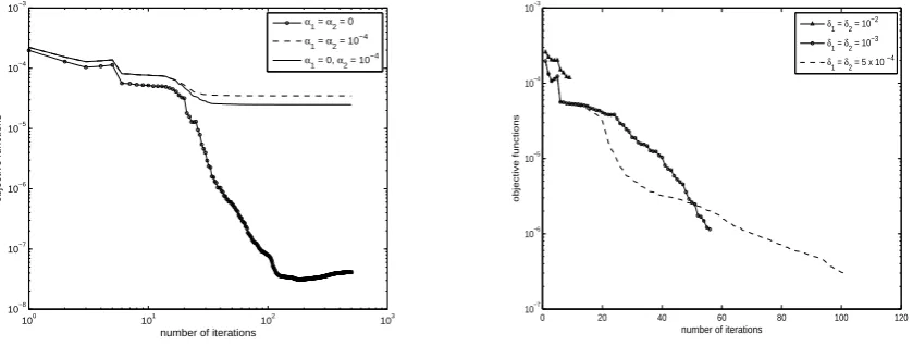
Figure 1: The objective functions without noise (left) and with noise (right) for Example 1.

Example 2. The exact solution is

f1(x) = sin(2πx1) sin(3πx2), f2(t) =

{

1 ift∈[1/3,2/3],

100 101 102 103 10−2

10−1

100

number of iterations

||f

1

−f

1h

|| L

2(Ω

)

α1 = α2 = 0

α1 = α2 = 10 −4

α1 = 0, α2 = 10 −4

100 101 102 103

10−3

10−2

10−1

number of iterations

||f

2

− f

2

τ

|| L

2(0,T)

α1 = α2 = 0

α1 = α2 = 10 −4

α1 = 0, α2 = 10 −4

Figure 2: The errors∥f1−f1h∥L2_(Ω) (left) and∥f₂−f_2τ∥_L2_(0,T) (right) without noise for Example

1. 0 0.2 0.4 0.6 0.8 1 0 0.2 0.4 0.6 0.8 1 −1 −0.5 0 0.5 1 x 1 x 2 f1 (x) 0 0.2 0.4 0.6 0.8 1 0 0.2 0.4 0.6 0.8 1 −1 −0.5 0 0.5 1 x 1 x 2 f1h (x) 0 0.2 0.4 0.6 0.8 1 0 0.2 0.4 0.6 0.8 1 −1.5 −1 −0.5 0 0.5 1 x₁ x₂ f1h (x) 0 0.2 0.4 0.6 0.8 1 0 0.2 0.4 0.6 0.8 1 −1 −0.5 0 0.5 1 x 1 x 2 f1h (x)

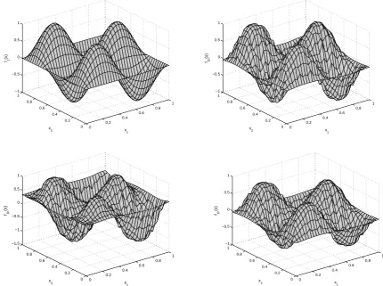
Figure 3: The exact solution f1(x) (top left) and the approximate solutions f1h(x) without noise

obtained with α1 = α2 = 0 (top right), α1 = α2 = 10−4 (bottom left), and α1 = 0, α2 = 10−4

0 0.2

0.4 0.6

0.8 1

0 0.2 0.4 0.6 0.8 1 −1 −0.5 0 0.5 1

x

1

x

2

f1h

(x)

0 0.2

0.4 0.6

0.8 1

0 0.2 0.4 0.6 0.8 1 −1 −0.5 0 0.5 1 1.5

x

1

x

2

f1h

(x)

Figure 4: The approximate solutionsf1h(x) with noiseδ1=δ2 = 5×10−4(left) andδ1 =δ2 = 10−3

(right) for Example 1.

0 0.1 0.2 0.3 0.4 0.5 0.6 0.7 0.8 0.9 1 −1.5

−1 −0.5 0 0.5 1

x₁

f1h

(x

1

,0.5)

Exact

α1 = α2 = 0

α1 = α2 = 10 −4

α1 = 0, α2 = 10 −4

0 0.1 0.2 0.3 0.4 0.5 0.6 0.7 0.8 0.9 1 −1

−0.5 0 0.5 1 1.5

x₁

f1h

(x

1

,0.5)

Exact

δ1 = δ2 = 10 −2

δ1 = δ2 = 10 −3

δ1 = δ2 = 5 x 10 −4

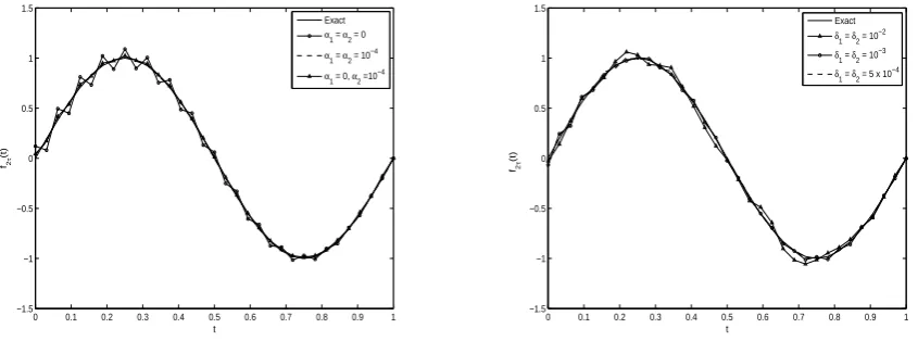
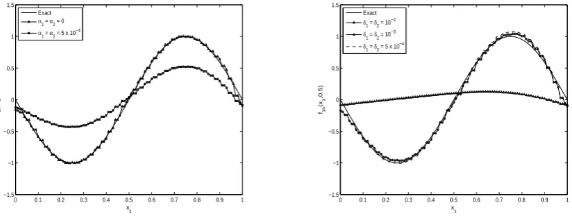
Figure 5: The approximate solutions f1h(x1,0.5) without noise (left) and with noise (right) for

Example 1.

0 0.1 0.2 0.3 0.4 0.5 0.6 0.7 0.8 0.9 1 −1.5

−1 −0.5 0 0.5 1 1.5

t

f2τ

(t)

Exact

α1 = α2 = 0

α1 = α2 = 10 −4

α₁ = 0, α₂ =10−4

0 0.1 0.2 0.3 0.4 0.5 0.6 0.7 0.8 0.9 1 −1.5

−1 −0.5 0 0.5 1 1.5

t

f2τ

(t)

Exact

δ1 = δ2 = 10 −2

δ1 = δ2 = 10 −3

δ1 = δ2 = 5 x 10 −4

Figure 6: The approximate solutionsf2τ(t) without noise (left) and with noise (right) for Example

100

101

102

103

10−8 10−7

10−6 10−5 10−4

10−3 10−2

number of iterations

objective functions

α1 = α2 = 0

α₁ = α₂ = 5x10−4

0 10 20 30 40 50 60 70 80 90 100 10−7

10−6

10−5 10−4

10−3 10−2

number of iterations

objective functions

δ1 = δ2 = 10 −2

δ1 = δ2 = 10 −3

δ₁ = δ₂ = 5 x 10−4

Figure 7: The objective functions without noise (left) and with noise (right) for Example 2.

100 101 102 103

10−1 100

number of iterations

||f1

− f

1h

|| L

2(Ω

)

α1 = α2 = 0

α1 = α2 = 5 x 10 −4

100 101 102 103

10−1 100

number of iterations

||f

2

− f

2

τ

|| L

2(0,T)

α1 = α2 = 0

α1 = α2 = 5 x 10 −4

Figure 8: The errors∥f1−f1h∥L2_(Ω) (left) and∥f₂−f_2τ∥_L2_(0,T) (right) without noise for Example

2.

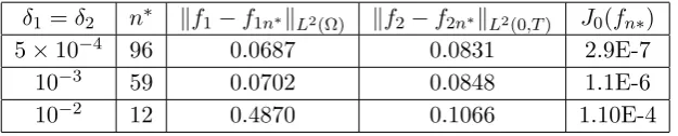
δ1 =δ2 n∗ ∥f1−f1n∗∥L2_(Ω) ∥f₂−f_2n∗∥_L2_(0,T) J₀(f_n∗)

5×10−4 96 0.0687 0.0831 2.9E-7

10−3 59 0.0702 0.0848 1.1E-6

10−2 12 0.4870 0.1066 1.10E-4

0 0.2 0.4 0.6 0.8 1 0 0.2 0.4 0.6 0.8 1 −1 −0.5 0 0.5 1 x 1 x 2 f1h (x) 0 0.2 0.4 0.6 0.8 1 0 0.2 0.4 0.6 0.8 1 −0.8 −0.6 −0.4 −0.2 0 0.2 0.4 0.6 x 1 x 2 f1h (x)

Figure 9: The approximate solutions f1h(x) without noise obtained with α1 = α2 = 0 (left) and

α1 =α2 = 5×10−4 (right) for Example 2.

0 0.2 0.4 0.6 0.8 1 0 0.2 0.4 0.6 0.8 1 −1 −0.5 0 0.5 1 1.5 x 1 x 2 f1h (x) 0 0.2 0.4 0.6 0.8 1 0 0.2 0.4 0.6 0.8 1 −1 −0.5 0 0.5 1 1.5 x 1 x 2 f1h (x)

Figure 10: The approximate solutions f1h(x) with noise: δ1 =δ2 = 5×10−4 (left) and δ1 =δ2 =

10−3 (right) for Example 2.

0 0.1 0.2 0.3 0.4 0.5 0.6 0.7 0.8 0.9 1 −1.5 −1 −0.5 0 0.5 1 1.5 x₁ f1h (x 1 ,0.5) Exact

α1 = α2 = 0

α1 = α2 = 5 x 10 −4

0 0.1 0.2 0.3 0.4 0.5 0.6 0.7 0.8 0.9 1 −1.5 −1 −0.5 0 0.5 1 1.5 x₁ f1h (x 1 ,0.5) Exact

δ₁ = δ₂ = 10−2

δ1 = δ2 = 10 −3

δ1 = δ2 = 5 x 10 −4

Figure 11: The approximate solutionsf1h(x1,0.5) without noise (left) and with noise α1 =α2 = 0

0 0.1 0.2 0.3 0.4 0.5 0.6 0.7 0.8 0.9 1 −0.2

0 0.2 0.4 0.6 0.8 1 1.2

t

f2τ

(t)

Exact

α1 = α2 = 0

α1 = α2 = 5 x 10 −4

0 0.1 0.2 0.3 0.4 0.5 0.6 0.7 0.8 0.9 1 −0.2

0 0.2 0.4 0.6 0.8 1 1.2

t

f2τ

(t)

Exact

δ1 = δ2 = 10 −2

δ₁ = δ₂ = 10−3

δ₁ = δ₂ = 5 x 10−4

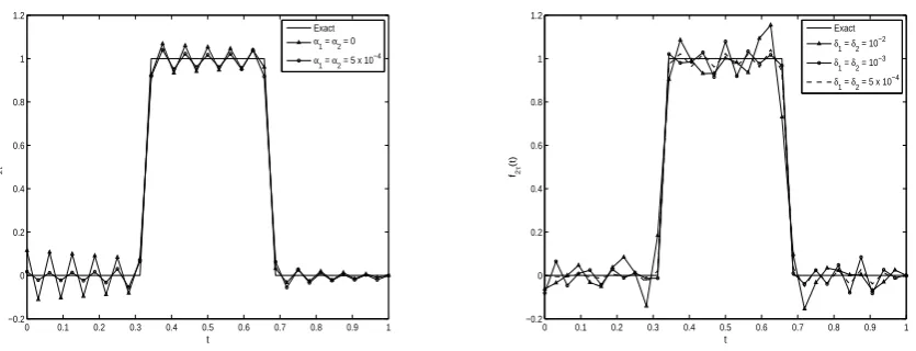
Figure 12: The approximate solutionsf2τ(t) without noise (left) and with noise (right) for Example

2.

Then C0 = 0. In this example, the function f1 is smooth, but f2 is discontinuous.

Example 3. The exact solution is

f1(x) =

{

1 ifx∈[0.3,0.7]2,

0 otherwise, f2(t) =

{

1 ift∈[1/3,2/3],

0 otherwise. (5.4)

Then C0 = 0.16. In this example, both functionsf1 and f2 are discontinuous.

5.1 Input Data Without Noise

We consider first the case of exact data, i.e. the input data (2.6) and (2.18) is without noise

δ1 =δ2 = 0.

The objective function (3.1) is plotted, as a function of the number of iterations, in the left hand

sides of Figures 1, 7 and 13 for Examples 1–3, respectively. Both cases of with, i.e. α ̸= 0, and

without, i.e. α= 0, regularization terms in (3.1) are illustrated. First, from these figures it can be

seen that for α ̸= 0, the objective function Jα rapidly decreases and settles at a stationary value

in about 20 iterations, showing that convergence has been achieved. Secondly, especially from the

left hand side of Figure 1 it can be seen that for α= 0 the objective functionJ0 rapidly decreases

for the first 100 iterations after which it starts increasing showing a semi-convergence phenomenon. This is expected since although we have no noisy random errors in the input data (2.6) and (2.18),

because we input the analytical values for g(x) and h(t), there will still exist a numerical ”noise”

generated by the use of a numerical discretization method with a fixed finite mesh size.

The behaviour of the errors ∥f1 −f1h∥L2_(Ω) and ∥f₂ −f_2τ∥_L2_(0,T), as functions of the number

of iterations, are shown in Figures 2, 8 and the right-hand side of Figures 13 for Examples 1–3,

respectively. From these figures it can be seen that for α = 0, after about 100 iterations the

errors∥f1−f1h∥L2_(Ω) decrease, whilst the errors∥f₂−f_2τ∥_L2_(0,T) increase. On the other hand, we

can reverse this behaviour by including some regularization. This reveals an interesting balancing

phenomenon happening in the sum of the sources in (2.1), namely, increasing the accuracy inf1(x)

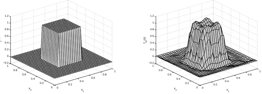
The numerical solutions f1h(x1, x2) are shown in comparison with the exact solutions f(x1, x2) in

Figures 3, 9 and 14 for Examples 1–3, respectively. From these figures it can be seen that there

is good agreement between the exact solutions and the numerical solutions obtained with α = 0.

Regularization withα ̸= 0 does not seem to improve further the accuracy of the numerical solutions

f1h(x1, x2). The above conclusion is more clearly illustrated by taking a slice through the plane

x2 = 0.5 and comparing in the left-hand sides of Figures 5, 11 and 16 the numerical solutions

f1h(x1,0.5) with the exact solutions f1(x1,0.5) for Examples 1–3, respectively. Finally, the

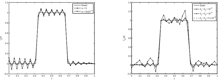
left-hand sides of Figures 6, 12 and 17 show the numerical solutionsf2τ in comparison with the exact

solutionsf2(t) for Examples 1–3, respectively. From these figures it can be seen that the numerical

solutionf2τ(t) obtained with no regularization, i.e.α= 0, is slightly oscillatory, but this instability

can be alleviated by the inclusion of some small regularization with α ̸= 0. Finally, we wish to

mention that in the case of input data without noise the choice ofα̸= 0 is irrelevant since most of

the results are stable and accurate as obtained using α = 0, and in any case, the stability of the

numerical solutions should be tested for noisy data, as described in the next subsection.

5.2 Input Data With Noise

We next consider the case of noise data, i.e. the input data (2.6) and (2.18) is contaminated by some

random noiseδ1 =δ2 ∈ {5×10−4,10−3,10−2} which is introduced in order to test the stability of

the numerical solution, as well as to model the errors which are inherently present in any practical

measurement. In this case, we can take α = 0, but then we will stop the CGM according to the

stopping rule (5.1).

The stopping iteration numbersn∗, the errors∥f1−f1n∗∥L2_(Ω)and ∥f₂−f_n∗∥_L2_(0,T) and the values

of the objective function J0(fn∗) are given in Tables 1–3 for Examples 1–3, respectively. The

decreasing monotonic behaviour of J0(fn), as a function of the number of iterations n, is also

illustrated in the right-hand sides of Figures 1 and 7 for Examples 1 and 2, respectively. From

these tables and figures it can be seen, as expected, that the stopping iteration number n∗(δ) is a

decreasing function of the amount of noise δ. Also, the numerical results become more accurate

and the objective function J0 decreases as the amount of noise δ decreases. Finally, we observe

that the values of n∗ are relatively small which show that the CGM is a much faster regularizing

algorithm compared to other much slower iterative algorithms such as the Landweber method for example.

For δ1 =δ2∈ {5×10−4,10−3}noise, the numerical solutions f1h(x1, x2) are shown in comparison

with the exact solutions f(x1, x2) in Figures 4, 10 and 15 for Examples 1–3, respectively. From

these figures it can be seen that the numerical solutions are stable and reasonably accurate. The

numerical results for a larger amount of noise such as δ1 =δ2 = 10−2 are not illustrated in these

figures because the numerical solutions obtained in this case were oversmoothed by the discrepancy principle (5.1). All these conclusions are further clearly illustrated in the right-hand side of Figures 5, 11 and 16 for Examples 1–3, respectively.

Finally, the results presented in the right-hand sides of Figures 6, 12 and 17 for Examples 1–3,

respectively, show that the numerical solutionsf2τ(t) are stable and reasonably accurate predictions

of the exact solutionsf2(t) for all the amounts of noise considered. We also observe that there is no

significant dependence (ont) of the numerical results astincreases, vis-a-vis of the local uniqueness

δ1 =δ2 n∗ ∥f1−f1n∗∥L2_(Ω) ∥f₂−f_2n∗∥_L2_(0,T) J₀(f_n∗)

5×10−4 123 0.1586 0.0829 2.98E-7

10−3 60 0.1760 0.0848 1.18E-6

10−2 13 0.2966 0.1133 1.06E-4

Table 3: The results for Example 3 with noise.

100

101

102

103

10−8 10−7 10−6

10−5 10−4

10−3

10−2 10−1

number of iterations

objective functions

α1 = α2 =0

α1 = α2 = 5x10 −4

100

101

102

103

10−1 100

number of iterations

Errors

||f₁ − f_1h|| _L2_(Ω), α1 = α2 = 0

||f₁ − f_1h|| _L2_(Ω), α1 = α2 = 5 x 10 −4

||f₂ − f_2τ|| _L2_(0,T), α1 = α2 = 0

||f₂ − f_2τ|| _L2

(0,T), α1 = α2 = 5 x 10

−4

Figure 13: The objective functions (left) and the L2-errors (right) for Example 3 without noise.

0 0.2

0.4 0.6

0.8 1

0 0.2 0.4 0.6 0.8 1 −0.2 0 0.2 0.4 0.6 0.8 1 1.2

x₁ x₂

f1

(x)

0 0.2

0.4 0.6

0.8 1

0 0.2 0.4 0.6 0.8 1 −0.2 0 0.2 0.4 0.6 0.8 1 1.2

x

1

x

2

f1h

(x)

Figure 14: The exact solution f1(x) (left) and the approximate solution f1h(x) without noise

0 0.2 0.4 0.6 0.8 1 0 0.2 0.4 0.6 0.8 1 −0.2 0 0.2 0.4 0.6 0.8 1 1.2 1.4 x 1 x 2 f1h (x) 0 0.2 0.4 0.6 0.8 1 0 0.2 0.4 0.6 0.8 1 −0.2 0 0.2 0.4 0.6 0.8 1 1.2 x 1 x 2 f1h (x)

Figure 15: The approximate solutionsf1h(x) with noiseδ1=δ2 = 5×10−4 (left) andδ1 =δ2 = 10−3

(right) for Example 3.

0 0.1 0.2 0.3 0.4 0.5 0.6 0.7 0.8 0.9 1 −0.2 0 0.2 0.4 0.6 0.8 1 1.2 x₂ f1h (0.5,x 2 ) Exact

α1 = α2 = 0

α1 = α2 = 5 x 10 −4

0 0.1 0.2 0.3 0.4 0.5 0.6 0.7 0.8 0.9 1 −0.2 0 0.2 0.4 0.6 0.8 1 1.2 1.4 x₂ f1h (0.5,x 2 ) Exact

δ1 = δ2 = 10 −2

δ1 = δ2 = 10 −3

δ1 = δ2 = 5 x 10 −4

Figure 16: The approximate solutions f1h(x1,0.5) without noise (left) and with noise (right) for

Example 3.

0 0.1 0.2 0.3 0.4 0.5 0.6 0.7 0.8 0.9 1 −0.2 0 0.2 0.4 0.6 0.8 1 1.2 t f2 (t) Exact

α = 0

α = 5x10−4

0 0.1 0.2 0.3 0.4 0.5 0.6 0.7 0.8 0.9 1 −0.2 0 0.2 0.4 0.6 0.8 1 1.2 1.4 t

f2τ

(t)

Exact

δ1 = δ2 = 10 −2

δ1 = δ2 = 10 −3

δ1 = δ2 = 5 x 10 −4

Figure 17: The approximate solutionsf2τ(t) without noise (left) and with noise (right) for Example

6

Conclusions

A novel inverse heat source problem with integral observations has been investigated. The local existence and uniqueness of a classical solution have been established and furthermore, a variational formulation has been proposed. The numerical method for obtaining a stable solution was based on the FEM combined with the CGM. The numerical results demonstrate that accurate and stable numerical solutions can be obtained. There seems to be a balance between predicting simultane-ously the space and time-dependent components of the additive source. Moreover, as expected, the reconstruction of the multi-dimensional space component is more difficult than the single-dimension time component of the source. Future work may consist into developing the analysis of this study for recovering a heat source which separates as the product, rather than sum, of two unknown functions; one which depends on space and one which depends on time. However, in this situation the inverse problem becomes nonlinear and the details appear more complicated. All the above programme builds upon ultimately attacking the challenging inverse problem of retrieving a heat source which depends on both space and time variables in a general way.

Acknowledgements

This research was supported by a Marie Curie International Incoming Fellowship within the 7th European Community Framework Programme, the London Mathematical Society, and by Vietnam National Foundation for Science and Technology Development (NAFOSTED) under grant number 101.02-2011.50.

References

[1] El Badia A. and Ha-Duong T., On an inverse source problem for the heat equation. Application

to a pollution detection problem.J. Inverse Ill-Posed Probl.10(2002), 585–599.

[2] Evans L.C.,Partial Differential Equations, Amer. Math. Soc., Providence, Rhode Island, 2002.

[3] Farcas A. and Lesnic D., The boundary-element method for the determination of a heat source

dependent on one variable.J. Engrg. Math.54(2006), 375–388.

[4] Gol’dman N.L., Properties of solutions of parabolic equations with an unknown right-hand

side and of their conjugate problems.Dokl. Math.77(2008), 350–355.

[5] Hanke M., Conjugate Gradient Type Methods for Ill-Posed Problems. Longman Scientific &

Technical, Harlow, 1995.

[6] Dinh Nho H`ao, Phan Xuan Thanh, Lesnic D., and Johansson B.T., A boundary element

method for a multi-dimensional inverse heat conduction problem. Int. J. Comput. Math.

89(2012), 1540–1554.

[7] Hasanov A. and Pektas B., Identification of an unknown time-dependent heat source term

from overspecified Dirichlet boundary data by conjugate gradient method. Comput. Math.

[8] Hasanov A. and Slodicka M., An analysis of inverse source problems with final time

mea-sured output data for the heat conduction equation: a semigroup approach.Appl. Math. Lett.

26(2013), 207–214.

[9] Hinze M. A variational discretization concept in control constrained optimization: The

linear-quadratic case,Computat. Optimiz. Appl., 30(2005), 45–61.

[10] Isakov V., Inverse Problems for Partial Differential Equations.Second edition. Springer, New

York, 2006.

[11] Ivanchov M.I., Inverse problem for a multidimensional heat equation with an unknown source

function.Mat. Stud. 16(2001), 93–98.

[12] Johansson B.T. and Lesnic D., A variational method for identifying a spacewise-dependent

heat source.IMA J. Appl. Math.72(2007), 748–760.

[13] Johnson C., Numerical Solution of Partial Differential Equations by the Finite Element

Method.Cambridge University Press, Cambridge, 1987.

[14] Ladyzhenskaya O.A., Solonnikov V.A., and Ural’ceva N.N.,Linear and Quasilinear Equations

of Parabolic Type, AMS, Providence, 1967.

[15] Nemirovskii A.S., The regularizing properties of the adjoint gradient method in ill-posed

prob-lems.Zh. vychisl. Mat. mat. Fiz.26(1986), 332–347. Engl. Transl. inU.S.S.R. Comput. Maths.

Math. Phys., 26(2)(1986), 7–16.

[16] Plato R., The conjugate gradient method for linear ill-posed problems with operator

pertur-bations. Numer. Algorithms20(1999), 1–22.

[17] Prilepko A.I. and Solov’ev V.V., Solvability theorems and the Rothe method in inverse

prob-lems for an equation of parabolic type. I.Differential Equations23(1987), 1230–1237.

[18] Prilepko A.I. and Tkachenko D.S., Inverse problem for a parabolic equation with integral

overdetermination.J. Inverse Ill-Posed Probl.11(2003), 191–218.

[19] Rundell W., Determination of an unknown nonhomogeneous term in a linear partial differential

equation from overspecified boundary data.Applicable Anal.10(1980), 231–242.

[20] Savateev E.G., On problems of determining the source function in a parabolic equation. J.

Inverse Ill-Posed Probl.3(1995), 83–102.

[21] Tr¨oltzsch F.,Optimale Steuerung partieller Differentialgleichungen, Vieweg + Teubner,