City, University of London Institutional Repository
Citation
:
Hunt, A. and Blake, D. (2017). Identifiability, cointegration and the gravity model. Insurance: Mathematics and Economics, doi: 10.1016/j.insmatheco.2017.09.014This is the accepted version of the paper.
This version of the publication may differ from the final published
version.
Permanent repository link:
http://openaccess.city.ac.uk/18374/Link to published version
:
http://dx.doi.org/10.1016/j.insmatheco.2017.09.014Copyright and reuse:
City Research Online aims to make research
outputs of City, University of London available to a wider audience.
Copyright and Moral Rights remain with the author(s) and/or copyright
holders. URLs from City Research Online may be freely distributed and
linked to.
City Research Online: http://openaccess.city.ac.uk/ [email protected]
Identifiability, Cointegration and the Gravity
Model
Andrew Hunt
∗Cass Business School, City University London
Corresponding author: [email protected]
David Blake
Pensions Institute, Cass Business School, City University London
July 2017
Abstract
The gravity model of Dowd et al. (2011) was introduced in or-der to achieve coherent projections of mortality between two related populations. However, this model as originally formulated is not well-identified since it gives projections which depend on the arbitrary identifiability constraints imposed on the underlying mortality model when fitting it to data. In this paper, we discuss how the gravity model can be modified to give well-identified projections of mortality rates and how this result can be generalised to more complicated mor-tality models.
JEL Classification: C32
Keywords: Mortality modelling, age/period/cohort models,
multi-population modelling, coherent mortality projection
∗We are grateful to Bent Nielsen and Michele Bergamelli for discussions regarding
1
Introduction
Hunt and Blake (2015b) and Hunt and Blake (2015c) discussed the issue of identifiability in single population age/period/cohort (APC) mortality mod-els, and in particular how to obtain projections of mortality rates which do not depend upon the arbitrary identifiability constraints imposed.
Issues with identifiability in projections also exist if we project mortal-ity for multiple populations rather than just one. Such multi-population projections are vital in order to allow for the correlations and dependencies between related populations that are influenced by similar biological and socio-economic drivers of changing mortality. It is essential that, in such a model, our projections do not depend on the arbitrary identifiability con-straints imposed when fitting the model, but only on the underlying drivers of mortality evolution.
Many multi-population mortality models go beyond merely allowing for covariation between the stochastic evolution of mortality in different popula-tions, and instead impose the stronger assumption of “coherence”, i.e., that mortality rates in different populations should not diverge with time. Such an imposition is popular and intuitively appealing; however, we find that it usually cannot be imposed on a model in a fashion which does not depend on the arbitrary identifiability constraints. In addition, it can often lead to overriding the evidence from the historical data in order to impose our pre-conceptions on projected mortality rates in a manner which we consider to be unscientific.
im-posed by the user.
In this study, we discuss the issue of identifiability in cointegration models and apply this to the specific context of the gravity model in order to obtain a well-identified model. Section 2 discusses the classic APC model which was used in Dowd et al. (2011) to fit mortality rates in both populations. Section 3 outlines the gravity model introduced in Dowd et al. (2011) and places it in the context of more general cointegration models. Section 4 discusses why the gravity model is not well-identified and how it can be modified to give well-identified projections. Section 5 discusses the model of Zhou et al. (2014), how it differs from the gravity model of Dowd et al. (2011) and the issues with identifiability which are still present. Finally, Section 6 generalises these results to a broader class of mortality models and Section 7 concludes.
2
Identifiability in the classic APC model
The simplest APC model (referred to here as the “classic APC model”) has a long history and is widely used in the fields of medicine, epidemiology and sociology as well as in demography and actuarial science. It has the form in Equation 11
ln(µx,t) =αx+κt+γt−x (1)
The parameters in the classic APC model cannot be estimated uniquely by reference to the data alone. A model is fully identified when all the pa-rameters in it can be uniquely determined by reference to the available data. In contrast, the classic APC model is not fully identified because there exist different sets of parameters which will give the same fitted mortality rates and consequently the same goodness of fit for any data set.
We can see that this model is not fully identified, since if we use the transformations in Equations 2, 3 and 4 to obtain new sets of parameters, we do not change our fit to the data (we call such transformations “invariant”
1In this paper, we assume that ages, x, are in the range [1, X] and periods, t, are in
for this reason)
{αˆx,κˆt,ˆγy}={αx−a, κt+a, γy} (2) {αˆx,κˆt,ˆγy}={αx−b, κt, γy+b} (3) {αx,ˆ κt,ˆ ˆγy}={αx+cx, κt−ct, γy +cy} (4)
Because different sets of parameters give the same fit to the data, we cannot use the data to choose between them. Typically, we impose iden-tifiability constraints on the parameters in order to specify them uniquely. For instance, a commonly used set of identifiability constraints is P
tκt = 0,
P
ynyγy = 0 and
P
ynyγy(y −y¯) = 0.
2 We refer to these identifiability
constraints as “natural”, since they allow us to impose our interpretation of the demographic significance3 of the parameters onto the model. For exam-ple, the first two of these constraints mean that αx can be interpreted as an
“average” level of mortality at age x over the period, with κt and γy
repre-senting deviations from this average level. The third constraint requires that there are no deterministic linear trends within the fitted cohort parameters, since any linear trend has been arbitrarily assigned to the age and period effects. This is in line with the demographic significance we assign to the cohort parameters in Hunt and Blake (2015e), namely that the cohort pa-rameters should be centred around zero and should not show any long term trends. This means that cohort effects are interpreted as deviations in the mortality experienced by one cohort relative to that of adjacent years of birth.
However, it is important to note that these additional identifiability con-straints, although having a natural interpretation, are arbitrary and ad hoc. While they might allow us to interpret the parameters in terms of their de-mographic significance, this interpretation nevertheless depends entirely on the user’s judgement rather than on the underlying data. Of specific impor-tance in the context of this study, Dowd et al. (2011) used the constraints
P
tκt= 0,
P
ynyγy = 0 and a third constraint described in terms of
minimis-ing a tiltminimis-ing parameter δ, which can be written as P
x,t(x−x¯)γt−x = 0. The
2Here n
y is the number of observations of cohort y in the data and so Pynyγy = P
x,tγt−x, and a bar denotes the arithmetic mean of the variable over the relevant data
range, e.g., ¯y=X+1T−1P
yy= 0.5(X+T) .
3Demographic significance is defined in Hunt and Blake (2015e) as the interpretation of
impact of using either the “natural” or the Dowd et al. (2011) identifiability constraints when making projections is assessed in Section 4.3.
Since the identifiability constraint we choose to impose are arbitrary and do not affect the historical fitted mortality rates, they should also not affect the future projected mortality rates either. In consequence, we should obtain the same projected mortality rates for any set of identifiability constraints, including but not limited to the two discussed above. We say that models with this property are “well-identified”.
3
The gravity model
The “gravity” model was introduced in Dowd et al. (2011) in order to ob-tain mortality projections for two different populations which do not diverge with time.4 This model might be appropriate for a small population, such
as the lives in an annuity book or pension scheme, which is a subpopulation of a much larger population, such as a national population. The analogy the authors use is of the smaller population being like a planet in orbit around a star (the larger population).
The gravity model requires that the classic APC model of Equation 1 is fitted to two populations5 and the period functions projected using
κt(I) =ν(I)+κt(I−)1+(tI)
κ(tII) =ν(II)+κ(tII−1)+φ(κ(t−I)1 −κ(t−II1)) +(tII) (5)
The parameterφ∈[0,1) is designed to ensure that the difference,κt(I)−κ(tII), is stationary and, therefore, the period functions in the different populations
4This model is functionally equivalent to the model in Cairns et al. (2011), which differs
only in the presentation of the model and the techniques used to fit it to data. Therefore, the comments made in this note for the gravity model are also applicable to the model of Cairns et al. (2011).
5In Dowd et al. (2011), these were referred to as populations 1 and 2, with the period
and cohort functions numbered accordingly. To avoid confusion with the different period functionsκ(ti)for models with more than one age/period term fitted to a single population, we shall refer to the populations asIandII and label the period functionsκ(tI)andκ
(II)
t
do not diverge.
We can rewrite Equation 5 as
∆ κ
(I)
t κ(tII)
!
=
ν(I)
ν(II)
+ 0 φ
1 −1 κ
(I)
t−1
κ(t−II1)
!
+
(I)
t (tII)
!
(6)
This model is just a special case of a more general cointegration model, although this interpretation was not commented upon in Dowd et al. (2011). A number of papers have suggested or implemented cointegration as a means of projecting the period parameters of mortality models for different popu-lations. Cointegration was first suggested in the work of Carter and Lee (1992), but was more recently used in the modelling of Li and Hardy (2011) and Yang and Wang (2013).
Cointegration between the period functions requires that we model the vector of time series processes as
∆κt =νXt+ p−1
X
i=1
Γi∆κt−i+ Πκt−p+t (7)
The rank of the matrix Π is then tested in order to identify the number of cointegrating relationships between the period functions in the model. If it is of rank r < N (the number of period functions in κt), then Π can be
decomposed as Π = αβ>, where α and β are N ×r matrices to give the interpretation that the rows of β>κt−p represent r stationary cointegrating
relationships between the different period functions. In order to use cointe-gration robustly, we need to ensure that any statements we make about the rank of Π are independent of our choice of identifiability constraints.
We can therefore see that the gravity model in Equation 6 has the same form as Equation 7, with p = 1, Xt = 1
, r = 1, α = 0, φ>
and
β = 1, −1>. The prescribed form for β imposes that there is a station-ary cointegrating relationship of the form κ(tI) −κ(tII) = Zt, and so ensures
that relative mortality rates will not diverge between the two populations, whilst the prescribed form for α allows the interpretation that population I
A related process was used in Dowd et al. (2011) to project the cohort parameters from the model. This can be written as
∆ γ
(I)
y γy(II)
!
=
µ(I)
µ(II)
+
α(I) 0
0 α(II)
∆ γ
(I)
y−1
γy(II−1)
! + 0 φ
1 −1 γ
(I)
y−1
γy(II−1)
!
+ ε
(I)
y ε(yII)
!
(8)
We can therefore see that this is also similar to the cointegration relationship in Equation 7.6
4
Identifiability in the gravity model
4.1
Period functions
The values of κ(tI) and κ(tII) are not uniquely identifiable by the classic APC model, but instead depend upon our choice of identifiability constraints. Equations 2 and 4 give us the freedom to add linear trends in time to ei-ther or both time series independently, i.e.
ˆ
κ(tII)
ˆ
κ(tII)
!
= κ
(I)
t κ(tII)
!
+
a(I)
a(II)
+
c(I)
c(II)
t
ˆ
κt=κt+a+ct (9)
However, this transformation, despite leaving the fitted mortality rates un-changed if we make the appropriate offsets to the static age functions and co-hort parameters, fundamentally alters the cointegration relationship in
Equa-6 There is a slight difference between Equation 8 and the standard form of the
coin-tegration relationship in Equation 7, in that Equation 8 involves a stationary term in
γy−1=γy(I−)1, γy(II−1)
>
tion 6 since
∆ˆκt= ∆κt+c
=ν +αβ>κt−1 +t+c
=ν +c−αβ>(a+ct) +αβ>κˆt−1+t
=νˆ−αβ>ct+αβ>κˆt−1+t
The transformed time series has a deterministic linear term, αβ>ct, which was not present in the original parameterisation. This means that the time series structure in Equation 6 is not well-identified. In practice, this has the consequence that the gravity model can be difficult to fit to historical time series and may give implausible values.
We might conjecture that a solution to this problem would be to allow for deterministic trends up to linear order in the cointegrating relationship, i.e., using ν0+ν1t in place ofν in Equation 6 to give
∆ κ
(I)
t κ(tII)
!
= ν
(I) 0
ν0(II)
!
+ ν
(I) 1
ν1(II)
!
t+
0
φ
1 −1 κ
(I)
t−1
κ(tII−1)
!
+
(I)
t (tII)
!
∆κt =ν0+ν1t+αβ>κt−1+t (10)
Such a model is well-identified as it does not change form under the transformation in Equation 9
∆ˆκt=ν0+ν1t+c−αβ>(a+ct) +αβ>κˆt−1+t
= ˆν0+ ˆν1t+αβ>κˆt−1+t
ˆ
ν0 =ν0+c−αβ>a
ˆ
ν1 =ν1−αβ>c
10 conflicts with our desire for biologically reasonable7 projections.
There is, however, a way to obtain both biological reasonableness and identifiability under the transformations in Equation 4. This is to restrict the linear deterministic trend in Equation 10 by imposing ν1 = αβ1 where
β1 is an arbitrary constant. This will ensure that the relevant deterministic
trend is present in κt, but is constrained within the stationary cointegrating
relationships and is not present in the non-stationary part of the relationship.
This means that we need to include constrained deterministic linear trends in the cointegrating relationship, but leave an unconstrained constant term, i.e.
∆κt=ν0+αβ1t+αβ>κt−1+t
=ν0+α(β>κt−1+β1t) +t (11)
To see that this structure is well-identified under the transformations in Equation 4, let us transform the parameters using Equation 9 to obtain
∆ˆκt=ν0+c−αβ>a+α β>κˆt−1+ (β1−β>c)t
+t
=νˆ0+α
β>κˆt−1+ ˆβ1t
+t
where νˆ0 = ν0 +c−αβ>a, as previously, and ˆβ1 =β1 −β>c. This model
also gives biologically reasonable values for φwhich do not depend upon the identifiability constraints imposed when fitting the models, as demonstrated in Section 4.3.
4.2
Cohort parameters
As with the period parameters, the values of γy(I) and γy(II) are not uniquely
identifiable in the classic APC model, but instead depend upon our choice of identifiability constraints. Equations 3 and 4 give us the freedom to add
7Introduced in Cairns et al. (2006) and defined as “a method of reasoning used to
linear trends in time to either or both time series independently, i.e.
ˆ
γy(II)
ˆ
γy(II)
!
= γ
(I)
y γy(II)
!
+
b(I)
b(II)
+
c(I)
c(II)
y
ˆ
γy =γy +b+cy (12)
Rewriting Equation 8 in the form
∆γy =µ+A∆γy−1+αβ>γy−1+εy
we see that this is also not well-identified as it changes form under the trans-formation in Equation 12
∆ˆγy =µ+c−Ac−αβ>(b+cy) +A∆ˆγy−1+αβ>γˆy−1+εy
as the transformed drift term, µˆ=µ+c−Ac−αβ>(b+cy), is now a linear function in year of birth, y.
However, in the same manner as used for the period parameters above, we can introduce a constrained linear trend into the cointegrating relationship in order to give well-identified projections which are biologically reasonable
∆γy =µ+A∆γy−1+α
β>γy−1+ ˜β1y
+εy (13)
This can be shown to be well-identified by transforming the cohort parame-ters in a similar fashion.
4.3
Application to England & Wales and CMI Assured
Lives data
for ages 50 to 90 and years 1947 to 2006.8
We start by fitting the classic APC model to the data.9 In doing so, we have a choice over the identifiability constraints imposed on the models for England & Wales and the CMI Assured Lives. We investigate four different sets of identifiability constraints, which were used for the classic APC model in Hunt and Blake (2015c), i.e.,
Case 1: P
tκt = 0,
P
ynyγy =
P
x,tγt−x = 0 and
P
ynyγy(y − y¯) =
P
x,tγt−x((t−t¯)−(x−x¯)) = 0.
Case 2: P
tκt = 0,
P
yγy = 0 and
P
yγy(y−y¯) = 0.
Case 3: P
tκt = 0,
P
x,tγt−x = 0 and
P
x,tγt−x(x−x¯) = 0.
Case 4: P
tκt = 0,
P
x,tγt−x = 0 and
P
x,tγt−x(t−¯t) = 0.
We investigate the constraints shown in Case 1 and Case 3 as they are the “natural” constraints and the constraints used in Dowd et al. (2011), respec-tively, as discussed in Section 2. The constraints in Case 2 are similar to those in Case 1, except that the summations are taken over each year of birth rather than over all ages and years in the dataset. This has the effect of moving from a weighted average of the cohort parameters being equal to zero (with the weights determined by the number of observations for each cohort) in Case 1 to a simple arithmetical average in Case 2, and similarly for the linear trend. Although not used for the classic APC model, similar constraints were imposed on the cohort term in Model M6 in Cairns et al. (2009) and so have been included for comparison. As discussed in Section 2, the logic underpinning the selection of the Case 3 constraints in Dowd
8Data for England & Wales is taken from Human Mortality Database (2014) and we
are indebted to the Continuous Mortality Investigation for providing providing the CMI Assured Lives dataset.
9To do this, we use a two-step procedure to fit the model for simplicity, i.e., we fit
et al. (2011) was that the static age function in the model should explain all the observed linearity across ages. We can apply similar logic to the period function in the classic APC model, i.e., that the period function, κt should explain all of the observed linearity across time, to give the constraints in Case 4.
It is important to note that all four sets of constraints were developed to give the same demographic significance to the cohort parameters, i.e., that they should be centred around zero and the other functions in the model should capture any linear trends. Because of this, these four sets of con-straints give very similar sets of fitted parameters when these are plotted. These sets of parameters also give identical fitted mortality rates, since they can be transformed into each other using Equations 2, 3 and 4. However, the different sets of parameters are not identical. We therefore see that demo-graphic significance, whilst helpful in selecting an appropriate set of identifi-ability constraints, does not specify a single, unique set of constraints to use. Model users with the same interpretation of the parameters can reasonably choose to impose different constraints and obtain different fitted parameters when using the same model with the same data. Furthermore, the fact that demographic significance is subjective and, in practice, different model users adopt a range of interpretations for the different parameters highlights the fact that we must take care to ensure that the projected mortality rates are independent of the arbitrary choice of constraints made when fitting the model, and underscores the extent to which the identifiability constraints we choose is arbitrary.
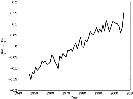
In each case, we apply the same identifiability constraints to both pop-ulations. Figure 1 shows the fitted values of κ(tI)−κ(tII) using the Case 1 constraints. Dowd et al. (2011) assumed that these differences are station-ary, however, Figure 1 shows that they have a clear linear trend which would bias the estimation of φ in the original specification of the model. Since the magnitude and direction of this trend is dependent upon the identifiability constraints imposed, the degree of this bias is dependent upon our choice of identifiability constraints. However, the modified gravity model allows for the potential presence of a linear trend in the cointegrating relationship and therefore any estimates for φ will not be biased by such a trend.
1940 1950 1960 1970 1980 1990 2000 2010 −0.2
−0.15 −0.1 −0.05 0 0.05 0.1 0.15 0.2
Year
κ
(EW) t
−
κ
[image:14.612.161.429.138.338.2](AL) t
Figure 1: Difference between the period functions
we then first fit the original gravity model in Equation 6 and then the mod-ified model in Equation 11. We pay particular attention to the estimated value ofφ found, as this will determine the rate at which divergence between the two populations mean reverts.
Original gravity model Modified gravity model
Case 1 0.0706 0.3234
Case 2 0.0702 0.3234
Case 3 0.0701 0.3234
Case 4 0.0700 0.3234
Table 1: Values of φ for different identifiability constraints
[image:14.612.149.461.471.547.2]same demographic significance for the parameters and therefore the fitted pa-rameters were broadly comparable. This will not necessarily always be the case, as demographic significance is subjective and different model users may have very different understandings as to the interpretation of the parameters.
The most important point is not how small the differences are but that they are different at all. The identifiability constraints made no difference to the the fitted mortality rates for the different cases - they were identical. However, the distribution of the projected mortality rates depends upon φ, which varies between the four cases in the original specification of the model. Therefore, the projected mortality rates would depend upon the choice of identifiability constraints. This is inconsistent with the fitting stage, where the choice of identifiability constraints made no difference to the fitted mor-tality rates. By contrast, the modified gravity model avoids this, as shown by the fitted value of φ being identical in all four cases in Table 1.
In particular, we note that it is possible that some sets of identifiability constraints for the classic APC model would give values of φ in the original gravity model which were greater than unity or less than zero. Therefore, the arbitrary choice of identifiability constraint may lead to diverging projections of mortality in the original gravity model, despite having the same historical fitted mortality rates as the cases shown. This is clearly something which should be avoided by use of the modified gravity model.
It is also interesting to note that the modified gravity model gives values for φ which are considerably larger than in the original model. This is be-cause the parameter now captures the genuine reversion between the period functions (i.e., the saw-tooth pattern in Figure 1) without additionally trying to capture the linear trend.
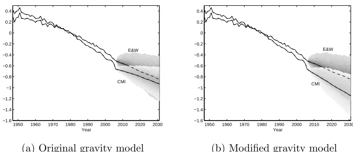
These modifications make a significant difference to the projected param-eters when using the gravity model, as shown in Figure 2 using the Case 1 identifiability constraints.
1950 1960 1970 1980 1990 2000 2010 2020 2030 −1.6
−1.4 −1.2 −1 −0.8 −0.6 −0.4 −0.2 0 0.2 0.4
Year
CMI E&W
(a) Original gravity model
1950 1960 1970 1980 1990 2000 2010 2020 2030 −1.6
−1.4 −1.2 −1 −0.8 −0.6 −0.4 −0.2 0 0.2 0.4
Year
E&W
CMI
[image:16.612.123.486.131.288.2](b) Modified gravity model
Figure 2: Projected period parameters
population to continue in future.
The change in trend exhibited by the period parameters in the original gravity model is explained by the transition between the past, where the linear trends are diverging in the period parameters fitted to the histori-cal data, and the future, where the gravity model is forcing them together. Since the linear trends in the fitted period parameters were unidentifiable and, hence, entirely dependent upon the identifiability constraints imposed upon the model, the magnitude of the trend change also depends solely upon the arbitrary identifiability constraints. Therefore, the existence of such a trend change is not well-identified and leads to projected mortality rates which depend upon the identifiability constraints chosen, unlike the fitted mortality rates.
believe that such an assumption is tenable.
In contrast, the modified gravity model does not predict a change in trend at the transition between past and future. As discussed in Hunt and Blake (2015c), the linear trends in the classic APC model are unidentifiable and depend entirely upon the identifiability constraints, whereas the variation around those trends is identifiable. Therefore, the modified gravity model leaves the linear trend in both populations unchanged, but allows the vari-ation around these trends to be cointegrated. This means that decreases in mortality which are faster than expected in England & Wales are correlated with faster than expected declines in mortality rates in the CMI Assured Lives population. Capturing this correlation is vital in the measuring of ba-sis risk between populations, as in Li and Hardy (2011) and Coughlan et al. (2011), and when modelling liabilities and securities which depend upon mor-tality in multiple populations, as discussed in Hunt and Blake (2015d).
Not only is the modified gravity model well-identified, we also believe that it gives projections which give greater consistency between the past and the future. The behaviour of the fitted parameters has been analysed and projected into the future, without assuming a priori that this behaviour will change. Such an approach is far more consistent with the extrapolative ap-proach to projecting mortality rates discussed in Section 2 of Hunt and Blake (2015a) than the assumption of a trend change present in the original gravity model.
Furthermore, we believe that an assumption whereby projections main-tain the same trends in each population but allow for correlated variation around these trends is more justified in terms of biological reasonableness than assuming that the period parameters converge in future. The fac-tors impacting deviations in mortality rates from trend in one population are likely to be common across populations, leading to correlated variation around the trend in the two populations. In contrast, the differing trend rates of mortality improvement are likely to be generated by more fundamen-tal socio-economic causes, which will remain unchanged for the foreseeable future.
popula-tions which are well-identified and have variation which is correlated in a biologically reasonable fashion. However, the modified gravity model does not induce the trends present in either population to change sharply at the transition point between past and future, which is a feature of the original gravity model and which was imposed to ensure that mortality rates in the two populations are “coherent”.
4.4
Coherence
The term “coherence” was introduced in Li and Lee (2005), and was defined formally in Hyndman et al. (2013) in terms of the relative mortality rates between populations, i.e.,
E
"
µ(p1)
x,t µ(p2)
x,t
#
→ Rx (14)
a function of age only. This means that relative mortality rates are stationary, and so the mortality rates projected in the two populations do not diverge with time. Coherence is a stronger requirement for a multi-population mor-tality model than simply allowing the covariation observed in the past to continue into the future, as discussed in Section 4.3 above.10
The original gravity model was introduced in part to ensure that mor-tality rates in the England & Wales and CMI Assured Lives populations are coherent. The original gravity model has coherence built into it, since
ln
"
µ(x,tI)
µ(x,tII)
#
= α(xI)−α(xII)+
κ(tI)−κ(tII)
+
γt(−I)x−γ
(II)
t−x
= α(xI)−αx(II)+β> κt+γt−x
which is stationary in time by construction.11
10Coherence is a potential feature of the projected mortality rates and can result from
a number of different techniques for projecting mortality, rather than it being a technique in itself. For instance, the original and modified gravity models both involve the technique of cointegration, but one gives coherent projected mortality rates, whilst the other does not. Conversely, the original gravity model and the SAINT model of Jarner and Kryger (2011) both give coherent mortality rates, but use different techniques to achieve this.
11However, the long-run distribution of µ(x,tI)
µ(x,tII), and specifically Rx, will depend upon the
However, when the gravity model is modified to ensure projections are well-identified, coherence no longer necessarily holds, since we can have differ-ent linear trends in both populations (i.e., β>κt+β1t+γt−x+ ˜β1(t−x)
is stationary, whilstβ> κt+γt−x
is not). The level of divergence will be set by the observed divergence between the populations in the historical dataset, i.e., we will project mortality rates that will continue to diverge if they have been observed to do so in the past. Such an approach gives greater consis-tency between the historical data and projected mortality rates.
Therefore, we see that there is the potential for conflict between the de-sire for coherent projections and the need for projections of the model to be well-identified. In general, we believe that obtaining projected mortality rates that do not depend on arbitrary choices made when fitting the model to data is more important than a desire to prevent divergence between popula-tions, for the reasons discussed below. However, we note that identifiability issues in mortality models are features of the parameters in mortality mod-els, whereas coherence is a property of the projected mortality rates, which should be independent of these issues. If coherence is desired, we therefore believe that methods of imposing it should focus on constraining the pro-jected mortality rates themselves, rather than specific features of the model parameters, which will depend on the identifiability constraints imposed.
However, we would often go further and question the desire to impose coherence a priori on projected mortality rates. Much of the work discussing coherent projections of mortality rates has been based on the idea that mor-tality rates should not diverge indefinitely in future between related popu-lations. For instance, Li and Lee (2005) stated that “Obviously, mortality differences between [closely related] populations should not increase over time indefinitely if the similar socio-economic conditions and close connections
were to continue.” We believe that there are two problems with this
conjec-ture.
arbitrarily close to zero at all ages if projected far enough into the future. However, such a phenomenon is more the fault of a modeller misusing the model to make inappropriate forecasts than it is the fault of the model it-self. A general rule of thumb is that a model should not be projected for a longer period than the data used to estimate it. Given this, the question becomes why we should believe that mortality differences cannot diverge for another 50 years (say) if we have observed mortality differences diverging for the previous 50 years. Assuming that the evolution of mortality rates in the future will be qualitatively different from the past is inconsistent with the extrapolative approach.
Second, we believe that it is simply untrue that differences in mortality rates cannot persist for prolonged periods between ostensibly related popu-lations. For example, life expectancy at age 65 varies considerably between areas in the same city12 in a pattern which has been stable for decades, let alone between different socio-economic groups within the same country (see Harper et al. (2007) and Villegas and Haberman (2014)) or between coun-tries. Whilst coherence does not impose the requirement that these long-established differences decrease, it does assume that they are not expected to grow beyond their current level, which we do not believe is supported by the evidence. It also raises the question as to what is so special about the currently observed differences in mortality that they should act as a barrier beyond which further divergence is not possible.
Therefore, we do not believe that coherence is a desirable property to im-pose upon an extrapolative multi-population mortality model. As scientific investigators, we should allow the data to speak for itself rather than impose any prior views onto the models that we use. This is consistent with the extrapolative approach discussed in Section 2 of Hunt and Blake (2015a), where analysis of historical data, rather than subjective opinions and biases, is used to project mortality rates. If the data supports our beliefs, that is encouraging. If the data does not, then we need to examine either our pre-conceptions to determine whether they need to be revised or re-examine the model we are using to analyse and project the data.
Ultimately, many of the preconceptions which lead to a desire for
herence between different populations have a basis in our knowledge of the specific populations under consideration and the specific factors causing the divergence in these populations. For example, the observed divergence be-tween mortality rates in the England & Wales and CMI Assured Lives popu-lations could be attributed to the selective nature of the CMI Assured Lives dataset, which consists of individuals who are likely to be wealthier than the average citizen of England & Wales. In addition, this selective population may adopt different lifestyles, with less smoking and a better diet than the wider population, for example, leading to a differing pattern of mortality. We might reasonably feel that such differences will get less important with time and the wider population adopts the same lifestyle as the sub-population, and therefore that mortality rates in the two population should stop diverg-ing in future.
However, this kind of argument for imposing coherence on a model makes use of additional information regarding the causes of any divergence, infor-mation that was not used when fitting the model. We therefore believe that, rather than imposing coherence on a model to obtain the results we want, it would be better to incorporate into our model the additional information that justifies our desire for coherence in the first place. Such information may include economic and lifestyle variables, for instance, as in Reichmuth and Sarferaz (2008), Wang and Preston (2009) and French (2014). This may help explain any observed divergence in the past and potentially allow for coherent projections which are still well founded in a rigorous analysis and extrapolation of the data.
5
Identifiability in the cointegrated Lee-Carter
model
Zhou et al. (2014) applied a similar cointegration framework as developed for the gravity model to the period parameters of the Lee-Carter model
ln(µx,t) =αx+βxκt (15)
series process of the form
∆κt=ν + Γ∆κt−1+αβ>κt−1+t (16)
which is a cointegrated relationship of the form in Equation 7.13 As in Dowd
et al. (2011), β was constrained so that β = 1, −1> in order that rel-ative mortality rates do not diverge in the two populations. However, no assumption is made regarding the dominance of one population over the other, and therefore no constraint is made on α, unlike the gravity model where α = 0, φ> was used to impose the condition that population I
dominates population II.
As discussed in Lee and Carter (1992) and Hunt and Blake (2015b), the Lee-Carter model is also not well-identified and possesses the invariant transformations
{αx,ˆ βx,ˆ κt}ˆ ={αx,1
aβx, aκt} (17) {αˆx,βˆx,κˆt}={αx−bβx, βx, κt+b} (18)
which are used to impose identifiability constraints in a similar fashion to the classic APC model. These invariant transformations can be applied indepen-dently to the two populations without affecting the fitted mortality rates, and so we can write
ˆ
κt=A(κt+b) (19)
with A=
a(I) 0 0 a(II)
.
If we apply this transformation to the time series process in Equation 16 we obtain
∆ˆκt =Aν−Aαβ>b+AΓA−1∆ˆκt−1+Aαβ>A−1κˆt−1+At
= ˆν + ˆΓ∆ˆκt−1+ ˆαβˆ>κˆt−1+ ˆt
13Again, the form of Equation 16 differs from the form of Equation 7 due to the
sta-tionary cointegrating term, αβ>κt−1, as opposed to αβ>κt−2 required by Equation 7.
which is of the same form as Equation 16 if we redefine the terms appropri-ately. In particular, this involves setting
ˆ
β=A−1β
=
1
a(I) 0
0 a(1II)
1
−1
= a(1I), −
1
a(II)
>
i.e., if the time series process is well-identified,β cannot be restricted to have any particular form, since these restrictions will only apply for one set of identifiability constraints. We also see that we are free to set ˆα =Aα, since
α is not constrained to any particular form initially. Therefore, in order for the model of Zhou et al. (2014) to be well-identified, the restriction on β as well as the restriction on αmust also be relaxed. This was commented upon in Nielsen and Nielsen (2014).
The reason for the difference between the models of Zhou et al. (2014) and Dowd et al. (2011) arises because of the differences in the underlying APC mortality models used in either study. In the Lee-Carter model used in Zhou et al. (2014), the “scale” of the period functions is defined by an identifiability constraint on βx. This scale is arbitrary, and we can change it without affecting the fitted mortality rates from the model. Therefore the projected mortality rates from the model of Zhou et al. (2014) also need to also be invariant to changes in this scale. In contrast, the scale of the pe-riod functions is defined by the parametric age function in the classic APC function, and not by an identifiability constraint. Therefore, it cannot be changed in the model, and so we do not have to ensure that the projected mortality rates are invariant to changes in its scale.
Conversely, the Lee-Carter model does not have unidentifiable linear trends, unlike the classic APC model. Therefore the model of Zhou et al. (2014) does not require a linear drift term, i.e., β1t, in the cointegrating
by the presence of the linear drift term,β1t, in the cointegrating relationships.
We see, therefore, that the form the gravity model needs to take in order to be well-identified depends on the underlying APC mortality model being used and the identifiability issues within that particular model. It is therefore essential that these identifiability issues are fully analysed and understood, as discussed in Hunt and Blake (2015b,c). In general, we see that it is best to avoid making any impositions on the structure of α and β, and so use the most general form of cointegrating relationship, in order to avoid any potential identifiability issues and avoid constraining the form of the model unnecessarily and, potentially, inappropriately.
6
Extending the cointegration model
For the general cointegration model in Equation 7, our approach generalises naturally to models where there are unidentifiable higher-order polynomial deterministic trends in the parameters. If the period functions of a model have unidentified deterministic trends which are polynomial of orderM, then in order to be well-identified under the corresponding invariant transforma-tions, we will need to allow for unconstrained deterministic trends up to polynomial order M −1 and constrained deterministic trends of orderM.
For instance, the model of Plat (2009)
ln(µ(x,tp)) =αx(p)+κt(1,p)+ (x−x¯)κt(2,p)+ (x−x¯)+κt(3,p)+γt(−p)x (20)
has unidentifiable quadratic trends, as discussed in Hunt and Blake (2015c). If the Plat (2009) model were fitted to two populations, we would have six pe-riod functions in total - κ(1t ,I) and κ(1t ,II) with unidentified quadratic trends,
κ(2t ,I) and κ(2t ,II) with unidentified linear trends and κ(3t ,I) and κ(3t ,II) with unidentified constants.
between all six time series would therefore mean allowing for constrained quadratic trends and unconstrained linear trends in all six period functions, which may lead to projections which are not biologically reasonable for each population.
It is more biologically reasonable to consider each pair of period func-tions separately based on their shared demographic significance. This would mean looking for cointegrating relationships with constrained quadratic (and unconstrained constant and linear) trends for the two κ(1t ,p) functions, rela-tionships with constrained linear trends for the κ(2t ,p) functions, and so on. That is, we use
∆κ(1)t =ν(1)0 +ν(1)1 t+α(1)
β(1)>κ(1)t−1+β2(1)t2
+(1)t (21)
∆κ(2)t =ν(2)0 +α(2)β(2)>κ(2)t−1+β1(2)t+(2)t (22)
∆κ(3)t =α(3)β(3)>κt(3)−1+β0(3)+(3)t (23)
to project the period functions. This approach is used in Hunt and Blake (2015d), albeit in a model with unidentified cubic (as opposed to merely quadratic) trends.
7
Conclusions
Cointegration can be a powerful tool for projecting mortality rates in related populations. However, it is a tool which must be used with care to ensure that we have identifiability under any invariant transformations which allo-cate unidentifiable polynomial trends between the parameters. In the case of the gravity model of Dowd et al. (2011) and the model of Zhou et al. (2014), we have shown how to adapt the process used to project the period functions so that it gives well-identified projections that do not depend on the arbitrary identifiability constraints imposed. We have also shown how this can be generalised to more complicated APC mortality models.
an extrapolative approach to modelling mortality. An extrapolative approach must, first and foremost, take its lead from the evidence of the historical data. While, in many circumstances, a belief in coherence is quite natural, we believe we should test for its existence in the historical data statistically using well-identified models, rather than assume its existence beforehand as an article of faith. If we do not find any evidence for coherence in the historical data, this should be considered a puzzle to explain using more data and better models, and not just an error to be corrected by an ad hoc fix which overrides the evidence of the data to obtain the results we anticipated in advance. Such an approach is not only more rigorous and more scientific, but can also give new insights into the factors which govern the evolution of mortality rates and enhance our understanding of longevity risk.
References
Cairns, A. J., Blake, D., Dowd, K., 2006. Pricing death: Frameworks for the valuation and securitization of mortality risk. ASTIN Bulletin 36 (1), 79–120.
Cairns, A. J., Blake, D., Dowd, K., Coughlan, G. D., Epstein, D., Ong, A., Balevich, I., 2009. A quantitative comparison of stochastic mortality models using data from England and Wales and the United States. North American Actuarial Journal 13 (1), 1–35.
Cairns, A. J., Blake, D., Dowd, K., Coughlan, G. D., Khalaf-Allah, M., 2011. Bayesian stochastic mortality modelling for two populations. ASTIN Bulletin 41 (1), 29–59.
Carter, R., Lee, D., 1992. Modeling and forecasting US sex differentials. International Journal of Forecasting 8, 393–411.
Coughlan, G. D., Khalaf-Allah, M., Ye, Y., Kumar, S., Cairns, A. J., Blake, D., Dowd, K., 2011. Longevity hedging 101: A framework for longevity ba-sis risk analyba-sis and hedge effectiveness. North American Actuarial Journal 15 (2), 150–176.
French, D., 2014. International mortality modelling - An economic perspec-tive. Economics Letters 122 (2), 182–186.
Harper, S., Lynch, J., Burris, S., Davey Smith, G., 2007. Trends in the black-white life expectancy gap in the United States, 1983-2003. The Journal of the American Medical Association 297 (11), 1224–32.
Human Mortality Database, 2014. Human Mortality Database. Tech. rep., University of California, Berkeley and Max Planck Institute for Demo-graphic Research.
URL www.mortality.org
Hunt, A., Blake, D., 2015a. Identifiability in age/period mortality models. Tech. rep., Pensions Institute PI 15-08, Cass Business School, City Uni-versity of London.
Hunt, A., Blake, D., 2015b. Identifiability in age/period/cohort mortality models. Tech. rep., Pensions Institute PI 15-09, Cass Business School, City University of London.
Hunt, A., Blake, D., 2015c. Modelling longevity bonds: Analysing the Swiss Re Kortis Bond. Insurance: Mathematics and Economics 63, 12–29.
Hunt, A., Blake, D., 2015d. On the structure and classification of mortality models. Tech. rep., Pensions Institute PI 15-06, Cass Business School, City University of London.
Hunt, A., Blake, D., 2016. Consistent mortality projections allowing for trend changes. Work in Progress.
Hyndman, R. J., Booth, H., Yasmeen, F., 2013. Coherent mortality fore-casting: The product-ratio method with functional time series models. Demography 50, 261–283.
Jarner, S. F., Kryger, E. M., 2011. Modelling mortality in small populations: The SAINT model. ASTIN Bulletin 41 (2), 377–418.
Lee, R. D., Carter, L. R., 1992. Modeling and forecasting U.S. mortality. Journal of the American Statistical Association 87 (419), 659– 671.
Li, N., Lee, R. D., 2005. Coherent mortality forecasts for a group of pop-ulations: An extension of the Lee-Carter method. Demography 42 (3), 575–594.
Nielsen, B., Nielsen, J. P., 2014. Identification and forecasting in mortality models. The Scientific World Journal, Article ID 347043.
Plat, R., 2009. On stochastic mortality modeling. Insurance: Mathematics and Economics 45 (3), 393–404.
Reichmuth, W., Sarferaz, S., 2008. Bayesian demographic modeling and fore-casting: An application to U.S. mortality. Tech. rep., Humbolt University, Berlin.
Villegas, A. M., Haberman, S., 2014. On the modeling and forecasting of socioeconomic mortality differentials: An application to deprivation and mortality in England. North American Actuarial Journal 18 (1), 168–193.
Wang, H., Preston, S. H., 2009. Forecasting United States mortality using cohort smoking histories. Proceedings of the National Academy of Sciences of the United States of America 106 (2), 393–8.
Yang, S. S., Wang, C.-W., 2013. Pricing and securitization of multi-country longevity risk with mortality dependence. Insurance: Mathematics and Economics 52 (2), 157–169.