A novel semi-supervised learning method based on fast search and density peaks

Research Article

A Novel Semi-Supervised Learning Method Based on

Fast Search and Density Peaks

Fei Gao ,

Teng Huang ,

Jinping Sun ,

Amir Hussain,

Erfu Yang,

and Huiyu Zhou

1_{School of Electronic and Information Engineering, Beihang University, Beijing 101191, China}

2_{Cognitive Big Data and Cyber-Informatics (CogBID) Laboratory, School of Computing, Edinburgh Napier University,} Edinburgh EH10 5DT, Scotland, UK

3_{Department of Design, Manufacture and Engineering Management, University of Strathclyde, Glasgow G1 1XJ, UK} 4_{Department of Informatics, University of Leicester, Leicester LE1 7RH, UK}

Correspondence should be addressed to Teng Huang; [email protected] and Jinping Sun; [email protected]

Received 5 October 2018; Revised 7 December 2018; Accepted 23 December 2018; Published 3 February 2019 Guest Editor: David Tom´as

Copyright © 2019 Fei Gao et al. This is an open access article distributed under the Creative Commons Attribution License, which permits unrestricted use, distribution, and reproduction in any medium, provided the original work is properly cited.

Radar image recognition is a hotspot in the field of remote sensing. Under the condition of sufficiently labeled samples, recognition algorithms can achieve good classification results. However, labeled samples are scarce and costly to obtain. Our major interest in this paper is how to use these unlabeled samples to improve the performance of a recognition algorithm in the case of limited labeled samples. This is a semi-supervised learning problem. However, unlike the existing semi-supervised learning methods, we do not use unlabeled samples directly and, instead, look for safe and reliable unlabeled samples before using them. In this paper, two new semi-supervised learning methods are proposed: a semi-supervised learning method based on fast search and density peaks (S2DP) and an iterative S2DP method (IS2DP). When the labeled samples satisfy a certain requirement, S2DP uses fast search and a density peak clustering method to detect reliable unlabeled samples based on the weighted kernel Fisher discriminant analysis (WKFDA). Then, a labeling method based on clustering information (LCI) is designed to label the unlabeled samples. When the labeled samples are insufficient, IS2DP is used to iteratively search for reliable unlabeled samples for semi-supervision. Then, these samples are added to the labeled samples to improve the recognition performance of S2DP. In the experiments, real radar images are used to verify the performance of our proposed algorithm in dealing with the scarcity of the labeled samples. In addition, our algorithm is compared against several semi-supervised deep learning methods with similar structures. Experimental results demonstrate that the proposed algorithm has better stability than these methods.

1. Introduction

Radar image recognition is a popular research area in the field of remote sensing [1–3]. With the development of imaging technologies and the expansion of radar image data, the requirement of real-time and accuracy of data processing becomes higher and higher. Under the condition where the number of the labeled samples is sufficient, a recognition algorithm can generally achieve satisfactory classification results with a strong sample representation ability [2, 4]. However, the labeled radar images are scarce compared to the case of optical images, and the cost of labeling is also very expensive. They can usually be interpreted by an experienced

expert [5, 6]. Therefore, it is unrealistic to obtain a large number of labeled samples by manual annotation.

This paper focuses on how to use these unlabeled samples to improve the performance of a recognition algorithm in the case of limited labeled samples. This is a semi-supervised learning problem. Currently, semi-supervised deep learning achieves promising recognition performance, such as Lad-der Network [7] and Temporal Ensembling [8]. However, unlike those existing semi-supervised learning methods, we do not use unlabeled samples directly and, instead, look for safe and reliable unlabeled samples and then use these unlabeled samples to enhance the performance of the recognition algorithm. This is because the unlabeled radar

images need to go through the detection stage in the process of acquisition [9, 10]. These samples may deteriorate the semi-supervised algorithms’ learning, especially when the number of the labeled samples and that of the unlabeled samples are somehow unbalanced. This will influence the performance of the semi-supervised algorithm. The negative effects of these unreliable and unlabeled samples on semi-supervised algorithms are analyzed comprehensively in [11, 12]. Therefore, it is very important for a semi-supervised algorithm to identify reliable unlabeled samples before we learn unlabeled samples’ features.

Effective use of unlabeled samples is a new and inter-esting topic for semi-supervised methods. These emerging semi-supervised methods are mainly divided into two cate-gories: semi-supervision based on integrated resources and safe semi-supervision based on weights. Semi-supervised methods, based on integration resources, usually combine multiple semi-supervised models, comprehensively analyse the predictions of unlabeled samples, and choose reliable unlabeled samples to improve the recognition performance

of the system. For example, Li et al. [13] proposed the S3

VM-us method, which consists of a semi-supervised support

vector machine (S3VM) [14] and a standard support vector

machine (SVM) [15]. The confidence of unlabeled samples is determined by both classifiers. If the evaluation results are consistent, the unlabeled samples are identified. Li et al. [16]

also proposed a safe S3VM method (S4VM). We understand

that the S3VM is based on the low-density hypothesis in

order to detect a significant interval along the low-density boundary from the feature space to identify unlabeled

sam-ples. Unlike S3VM, S4VM was based on the fact that there

may be more than one low-density boundary in the feature space. This approach considers all the possible situations,

equivalently, integrating multiple S3VMs to pinpoint reliable

unlabeled samples. Wang et al. [17] proposed a safety-aware semi-supervised method. It consists of a semi-supervised model and a supervised model, which minimized the square loss between the two models in order to detect reliable unlabeled samples. Similar to [17], Gan et al. [18] proposed a safe semi-supervised method which added a Laplace regularization term to the square loss function to enhance the reliability of unlabeled sample selection. Persello et al.

[19] proposed a progressive S3VM with diversity (PS3VM-D)

method. On the basis of multiple confidence measurements, reliable unlabeled samples were obtained by querying the samples nearby the margin band.

Weight-based semi-supervisory is based on the fact that the more unlabeled samples with similar weights to the label-ed samples, the more reliable the system becomes. Therefore, the influence of unreliable unlabeled samples on the algorith-mic performance is suppressed by reducing their weights. For example, [20] considered the unlabeled samples nearby the classification plane and suppressed their influence on the sys-tem performance by reducing their weights. In addition, [21– 23] controlled the weights by density estimation, weighted likelihood maximization, and graph modelling.

The above semi-supervised methods use unlabeled sam-ples to some extent, however, they also ignore the number of

the labeled samples. If the labeled samples are too few, the performance of these algorithms is difficult to be guaranteed, which will inevitably affect the evaluation of the reliability of unlabeled samples. In addition, they lack investigating variability and similarity between unlabeled and labeled samples, which makes it difficult to understand the dynamics and interaction of unlabeled samples. Therefore, in this paper, two new semi-supervised learning methods are proposed: a semi-supervised learning method based on fast search and

density peaks (S2DP) and an iterative S2DP method (IS2DP).

When the labeled samples satisfy a certain number, S2DP

is used directly to identify reliable unlabeled samples. For one thing, it works with a new sample weighted kernel Fisher discriminant analysis (WKFDA) supervision method. Using the difference between the samples, the WKFDA method extracts the features of the labeled samples to help formulate the distribution of the unlabeled samples’ features, solving the problem of mismatch between them. And for another, it is combined with a clustering method: fast search and determination of density peaks (DP) proposed by Rodriguez and Laio in 2014 [24]. Then, unlabeled sample features are further investigated so that the reliable unlabeled sample features are identified. Finally, an unlabeled sample labeling method based on clustering information (LCI) is designed to retrieve the labels of the unlabeled sample features.

When the labeled samples are insufficient, IS2DP is used

to iteratively render reliable unlabeled samples. Since the labeled and the unlabeled samples may be uneven in num-bers, the unreliable unlabeled samples tend to deteriorate

the semi-supervised algorithm. The IS2DP first divides the

unlabeled learning set into different subsets according to the size of the labeled sample set. This not only prevents the deterioration of the semi-supervised algorithm by a large number of unreliable samples but also speeds up the

processing of the semi-supervised algorithm. Then, the S3VM

is exploited to go through the semi-supervised samples which

may be away from the hyperplane of the S3VM as the reliable

semi-supervised samples are added to the labeled samples to improve the performance of the semi-supervised algorithm.

The rest of this paper is organized as follows. Section 2 gives a brief review of the approaches involved. Section 3 describes the proposed method in detail. Section 4 presents the experiments for the SAR images targets recognition. The conclusion is drawn in Section 5.

2. Preliminary

2.1. DP Algorithm. Clustering by fast search and detection of density peaks (DP)[24] can quickly realize accurate detection and clustering of various shapes. Moreover, it is used to evaluate each cluster membership so as to determine reliable cluster members. The DP algorithm is mainly divided into the following three steps.

(1) Determination of Cluster Centers. In the DP, it is assumed that the cluster centers are surrounded by the neighbors with the lower local density and they are at a relatively large distance from any points with a higher local density. Based

quantities are calculated: the local density𝜌_𝑖of the sample and

the distance𝜎_𝑖from a sample to the other with a high local

density. In the decision map with𝜌_𝑖and𝜎_𝑖as the horizontal

and vertical coordinates, respectively, their product is

𝛾_𝑖= 𝜌_𝑖𝜎_𝑖 (1)

where the sample point with the larger𝛾_𝑖is more likely to be

the cluster center. Therefore, only𝛾_𝑖is sorted in a descending

order, and several corresponding samples are selected as the clustering center from the largest value.

(2) Clustering of Samples. After the clustering center has been determined, all the samples are assigned to be the nearest cluster centers. Compared with the other clustering algorithms, DP clustering process is simple and does not require iterative optimization of the loss function.

(3) Automated Evaluation of Cluster Members. In the clus-tering results, it is important to quantitatively evaluate the credibility of each sample cluster. The DP algorithm has this capability, compared to other clustering algorithms. It firstly defines a neighbourhood for each cluster. Then, the

maximum value 𝜌_𝑏 of the local density of the samples is

found in each neighbourhood. Finally, in each cluster, all the

samples with local density greater than𝜌_𝑏are considered as

the cluster core candidates, otherwise, they are considered as the cluster halo of the cluster. The samples in the cluster core are very similar to the central samples and belong to reliable samples. The samples in the cluster halo have a certain distance from the central sample, which is very likely to be noise and belongs to unreliable samples. In addition, there are some cross-clustering and isolated samples that are also unreliable.

In summary, after having clustered by the DP, the samples located at the cluster core are considered to be reliable cluster samples, whilst the others are unreliable samples. Compared to the conventional clustering algorithms, such as Clara [25] or Fanny [26], the DP has lower computational complexity and less computational time. It also well characterizes the distribution of the samples and achieves more accurate clustering results. Besides, the reliability of the clustering results can be provided, which makes the DP easy to be interactive with other algorithms. However, only considering the distance between the sample points can insufficiently characterize the data because it cannot accurately describe the samples with small difference between two categories. When the sample dimension is high, the distance matrix is large, which can reduce the efficiency of the algorithm. Therefore, choosing the appropriate feature extraction method is a key in the DP.

2.2.𝑆3𝑉𝑀Method. The S3VM is the extension of the support vector machine (SVM). A standard SVM is based on the structural risk minimization to classify the learning set by extracting the support vectors from the training set to find the optimal hyperplane. In case of the binary SVM, given the

training setL and the testing setU, we have the following

constriction optimization problem:

min Φ (𝑤) = 1

2(𝑤𝑇𝑤) +

𝑛

∑

𝑖=1𝑐𝑖𝜉𝑖

𝑠.𝑡. y_𝑖[𝑤𝑇Φ (𝑥_𝑖) + 𝑏] ≥ 1 − 𝜉_𝑖,

𝜉𝑖≥ 0, i= 1, 2, ⋅ ⋅ ⋅ ,n

(2)

where𝑥_𝑖is the training sample and𝑦_𝑖is the corresponding

label, (𝑥_𝑖,𝑦_𝑖)∈ L;Φ(⋅) maps the data into the feature space;

𝑤is the orthogonal vector between𝑥_𝑖 and the hyperplane;

𝑏 is the bias to measure the distance between L and the

hyperplane;𝜉_𝑖is the slack variable to represent the offset of𝑥_𝑖;

𝑐_𝑖is the cost factor to measure the weight between the optimal

hyperplane and the minimum offset;𝑛is the number of the

training samples.

For the S3VM, the iterative process is operated and

the semi-labeled samples (selected fromUin the previous

step) are added toL. Their confidence is diverse in different

iterative steps and they are given different cost factors, leading to the following function:

min Φ (𝑤) = 1

2(𝑤𝑇𝑤) +

𝑛

∑

𝑖=1

𝑐_𝑖𝜉_𝑖+∑𝑚

𝑖=1

𝑐_𝑗𝜀_𝑗

𝑠.𝑡. y_𝑖[𝑤𝑇Φ (𝑥_𝑖) + 𝑏] ≥ 1 − 𝜉_𝑖,

𝜉𝑖≥ 0, i= 1, 2, ⋅ ⋅ ⋅ ,n ∧

𝑦_𝑗[𝑤𝑇Φ (𝑥∧_𝑗) + 𝑏] ≥ 1 − 𝜀_𝑗,

𝜀_𝑗≥ 0, j= 1, 2, ⋅ ⋅ ⋅ ,m (3)

where𝑥∧_𝑗is the semi-labeled sample selected fromU, with the

slack variable (𝜀_𝑗), cost factor (𝑐_𝑗) and semi-label (𝑦∧_𝑗) and𝑚

is the number of the semi-labeled samples.

The S3VM can deal with the nonlinear problem using

the kernel methods and its semi-supervised samples with

the bigger 𝑐_𝑗. But when the sample dimension is high, the

computation speed would decrease. Therefore, the dimension reduction and effective semi-supervised samples are the

critical aspects to the S3VM.

3. Proposed Methods

This paper presents two methods: S2DP and IS2DP. When

the labeled samples exceeds a certain number, S2DP directly

performs screening and classification of the reliable unlabeled

samples. When the labeled sample is insufficient, IS2DP is

used to continuously query reliable unlabeled samples and generate necessary samples to be added to the labeled samples

in order to improve the recognition performance of S2DP. The

S2DP and IS2DP are described below, respectively.

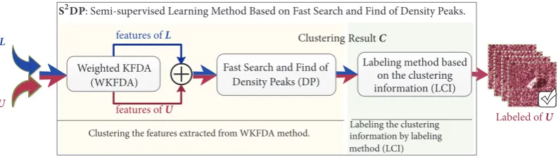
3.1. 𝑆2𝐷𝑃. Figure 1 shows the flowchart of the proposed

L

U

Clustering Result C

features of _U

features of L

SDP: Semi-supervised Learning Method Based on Fast Search and Find of Density Peaks.

Clustering the features extracted from WKFDA method.

Labeled of _U

Labeling the clustering information by labeling method (LCI)

Labeling method based on the clustering information (LCI) Fast Search and Find of

Density Peaks (DP) Weighted KFDA

(WKFDA)

Figure 1: Basic flowchart of the S2DP.

features to build a new space. New features are obtained by projecting unlabeled samples into this new space. In this space, the new feature distributions are as close as possible between the intraclass features with a certain weight, and the interclass features are as far apart as possible to enhance the separability between the features. Secondly, the DP is used to cluster the generated features. Finally, the unlabeled samples are identified by the labeling method based on the

DP clustering information (LCI). In Figure 1,L represents

a set of the labeled samples, andU represents a set of the

unlabeled samples, which respectively generate features with the labeled information (i.e., labeled features) and features without labeled information (i.e., unlabeled features) after

going through WKFDA;Crepresents the clustering results of

the DP. The WKFDA and LCI methods are described in the following section.

(1) WKFDA. Assume that𝑋represents all the samples of L

and the𝑖th category𝑋_𝑖 = [𝑥₁𝑖, 𝑥₂𝑖, . . . , 𝑥_𝑁𝑖𝑖]is the subset of𝑋,

where𝑁_𝑖is the samples’ number of𝑋_𝑖.𝑣_𝑖 = [V₁𝑖,V₂𝑖, . . . ,V_𝑁𝑖𝑖]

is the sample weight vector of 𝑋_𝑖. It is used to control

intraclass samples as close as possible with certain weights. In case of the binary classification, it cannot simply multiply the weight by the corresponding sample. Firstly, the

weight matrices𝑉_𝑖and𝐻_𝑖are generated:

𝑉_𝑖=diag(V₁𝑖,V₂𝑖, . . . ,V_𝑁

𝑖

𝑖₎

𝑁𝑖∗𝑁𝑖

𝐻_𝑖= [𝑣_𝑖,𝑣_𝑖, . . . ,𝑣_𝑖]_{𝑁𝑖∗𝑁𝑖} (4)

Secondly, the weight vector and the weight matrix are normalized using

𝑣_𝑖= 𝑣𝑖

𝑠𝑢𝑚 (𝑣_𝑖)

𝑉_𝑖= 𝑁𝑖𝑉𝑖

𝑠𝑢𝑚 (𝑉_𝑖)

𝐻_𝑖= 𝐻𝑖

𝑠𝑢𝑚 (𝐻_𝑖)

(5)

where𝑠𝑢𝑚(⋅)represents the summation. The above weight

matrix can be used to measure the information of the sample

itself. Although𝑉_𝑖and𝐻_𝑖are made up of𝑣_𝑖, their elements

are different. The sum of each column’s elements of𝐻_𝑖is equal

to 1, and the trace of𝑉_𝑖is equal to𝑁_𝑖. Thirdly, the projection

direction𝑤is calculated by Equation (6):

𝑤=∑𝑁

𝑗=1

𝑎_𝑗Φ (𝑥_𝑗)V_𝑗=∑𝑁

𝑗=1

𝑎_𝑗V_𝑗Φ (𝑥_𝑗) =∑𝑁

𝑗=1

𝛽_𝑗Φ (𝑥_𝑗)

= Φ (𝑋)𝛽

(6)

where𝛽_𝑗 = 𝑎_𝑗V_𝑗.Φ(⋅)is nonlinear mapping that maps the

samples to a new feature space. In this new space, the sample’s mean, before and after the projection has been made, can be calculated by

𝑚_𝑖𝜙= _𝑁1

𝑖

𝑁𝑖

∑

𝑗=1

Φ (𝑥𝑖_𝑗)V𝑖_𝑗= _𝑁1

𝑖Φ (𝑋𝑖)𝑣𝑖

𝑤𝑇𝑚_𝑖𝜙= _𝑁1

𝑖 𝑁

∑

𝑗=1

𝑁𝑖

∑

𝑘=1

𝛽_𝑗Φ (𝑥_𝑗) Φ (𝑥𝑖_𝑘)V𝑖_𝑘=_𝑁1

𝑖𝛽

𝑇_𝐾

𝑖𝑣𝑖

(7)

The interclass scatter matrix𝑤𝑇𝑆𝜙_𝑏𝑤and intraclass scatter

matrix𝑤𝑇𝑆𝜙_𝑤𝑤, after the projection has been achieved, are

calculated by

𝑤𝑇𝑆𝜙_𝑏𝑤=𝑤𝑇(𝑚𝜙₁−𝑚₂𝜙) (𝑚𝜙₁−𝑚₂𝜙)𝑇𝑤

=𝛽𝑇𝑀𝛽

𝑤𝑇𝑆𝜙_𝑤𝑤

=∑2

𝑖=1

𝑁𝑖

∑

𝑗=1

𝑤𝑇[Φ (𝑥𝑖_𝑗)V𝑖_𝑗−𝑚_𝑖𝜙] [Φ (𝑥𝑖_𝑗)V𝑖_𝑗−𝑚_𝑖𝜙]𝑇𝑤

=𝛽𝑇𝐺𝛽

(8)

where 𝑀 = (𝐾₁𝑣₁/𝑁₁ − 𝐾₂𝑣₂/𝑁₂)(𝐾₁𝑣₁/𝑁₁ −

𝐾₂𝑣₂/𝑁₂)Tand 𝐺 = ∑2_𝑖=1𝐾₁(𝑉_𝑖 − 𝐻_𝑖)(𝑉_𝑖 − 𝐻_𝑖)T𝐾_𝑖𝑇. In order to satisfy the requirements of the maximum interclass interval and the minimum intraclass interval, this goal can be expressed as follows:

max𝐽 (𝑤) = 𝛽

𝑇_𝑀𝛽

which is called the generalized Rayleigh quotient. Then 𝛽 can be calculated according to the flowchart of the KFDA by solving the following optimization problem:

max 𝛽𝑇𝑀𝛽

𝑠.𝑡. 𝛽𝑇𝐺𝛽= 𝑐 ̸= 0 (10)

where𝑐 is the constant. By introducing the Lagrange

mul-tiplier, the function can be transformed to a Lagrange unconstrained extremum problem:

𝐿 (𝑤, 𝜆) =𝛽𝑇𝑀𝛽− 𝜆 (𝛽𝑇𝐺𝛽− 𝑐) (11)

Let𝜕𝐿(𝑤, 𝜆)/𝜕𝛽= 0,𝜕(⋅)represent the partial derivative. This

function solution𝛽is the eigenvector of𝐺−1𝑀. Once solving

𝛽, for any sample𝑥, its projection is

𝑦 = ⟨𝑤, Φ (𝑥)⟩ =∑𝑁

𝑖=1

𝑎_𝑗V_𝑗𝑘 (𝑥_𝑖,𝑥) =𝛽𝑇𝐾_𝑥 (12)

where𝐾_𝑥is the kernel matrix of all the training samples and

𝑥.

Adding weights to KFDA algorithm is a common way to improve the KFDA algorithm. The aim is to make the WKFDA algorithm better learn sample features. However, different ways of adding weights make the WKFDA algorithm focus on learning sample features differently. For example, [27] added weights to each kernel function. The purpose was to introduce the prior knowledge of samples to enhance the learning of sample features in the WKFDA algorithm. Reference [28] added weights to the within-class scatter matrix. The purpose was to make the WKFDA algorithm not only learn the features of different types of samples but also learn the features of same types of samples in the process of finding the best vector. Unlike these algorithms, the WKFDA algorithm in this paper adds weights to samples, and these weights can be calculated by using the similarity or iterative difference of the samples. The purpose is to make the intraclass samples close to a certain distance, so that the WKFDA algorithm can not only suppress overfitting due to the small number of labeled samples but also facilitate the absorption of spectral information of samples to improve the learning of sample features. Although the binary WKFDA is shown, the multi-WKFDA can be obtained in accordance with the promotion of the kernel Fisher discriminant analysis (KFDA) [29].

(2) LCI. After the labeled sample setL and the unlabeled

sample setU have been extracted by the WKFDA method,

the labeled and unlabeled features are obtained. Next, the labeled and unlabeled features go into the DP to produce a

clustering resultC. The clustering resultC includes features

such as cluster center, clustering core, clustering halo, and cross-clustering, but is insufficient to determine the labels of the unlabeled features. To solve this problem, we develop the LCI by using the clustering results and labeling information of the labeled features. LCI is able to label the clustering results of the unlabeled features. Because the unlabeled features are

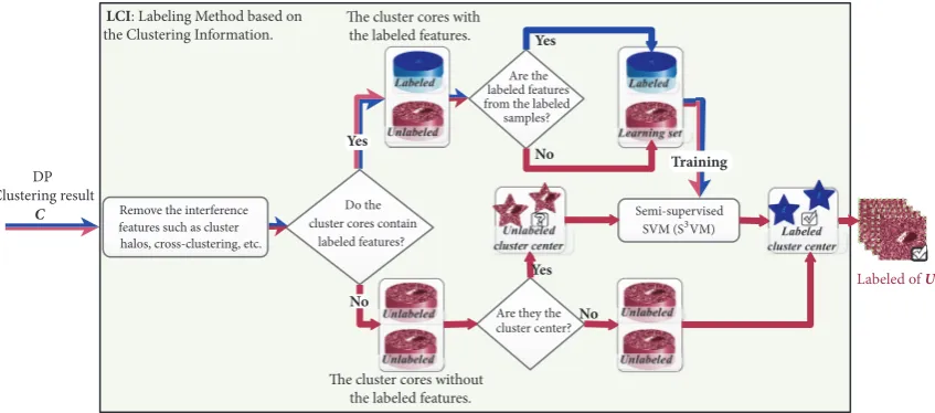
generated from the unlabeled samples, the unlabeled features and the unlabeled samples share the same labels. The basic flowchart of the LCI is shown in Figure 2.

We know that the features of clustering halo and cross-clustering are unreliable. Therefore, in Figure 2, the

inter-ference features inC need to be cleared to ensure that the

subsequent unlabeled features are reliable. TheCclearing the

interference is processed separately according to whether the labeled features are included in the cluster core. If there are labeled features in a certain cluster core, the unlabeled features of the cluster core are very similar to the labeled features. These unlabeled features are regarded as the best learning features, combined with the corresponding labeled

features, for training the S3VM. At this time, in each iteration

of the S3VM, the labeled features from the unlabeled features

are added to the next iteration to improve the robustness

of the S3VM algorithm. For the clustering cores which

do not contain any labeled feature, the cluster centers are

extracted and sent to the trained S3VM to obtain their labels.

Once the unlabeled cluster centers are labeled, the unlabeled features of the corresponding clustering core will be assigned the label. In this way, all the clustering cores’ features are labeled, and the features that are not labeled are removed as noise. Finally, the unlabeled samples corresponding to the unlabeled features also have corresponding labels.

3.2.𝐼𝑆2𝐷𝑃. When the number of the labeled samples is small

but reaches a certain amount, the S2DP uses the labeled

fea-tures to investigate the distribution of the unlabeled feafea-tures and also use the labeled features and the clustering result of the DP to obtain reliable unlabeled samples. However, when the number of the labeled samples is small, after the DP clustering has been achieved, the labeled features are not necessary in the cluster core, resulting in a low correlation between the labeled and unlabeled features. At this time, the labelled samples are difficult to represent the unlabeled

samples, and S2DP is no longer applicable. In this case, the

common solution is that the semi-labeled sample from the unlabeled set is queried in order to increase the number of the original labeled samples. In order to obtain the reliable

semi-labeled samples, the S2DP needs to be modified iteratively.

The iterative semi-supervised method of the S2DP,

namely, the IS2DP, is shown in Figure 3, whereU is the

unlabeled learning set to query the semi-labeled samples,L

is the labeled training set,𝐿∗is the semi-labeled samples set

in each iteration,𝐿󸀠represents the final labeled training set,

andTis the testing set.

The IS2DP specific process is described as follows. Firstly,

in each iteration,U is randomly divided into several

sub-sets (𝑈₁,𝑈₂, . . . ,𝑈_𝑛), which are combined withL to obtain

(𝑈₁,𝐿), (𝑈₂,𝐿),. . ., (𝑈_𝑛,𝐿) as the input of the S2DP. Secondly,

the cluster cores are selected from (𝑈₁,𝑈₂, . . . ,𝑈_𝑛) after the

S2DP as the candidate semi-labeled samples, and their cluster

centers are added to the training set as the labeled samples

to train S3VM. For one thing, the number of the labeled

LCI: Labeling Method based on

the Clustering Information.

the labeled features. The cluster cores without

Remove the interference

Are they the Do the

Are the

samples?

Semi-supervised labeled features

from the labeled

cluster cores contain labeled features?

cluster center? features such as cluster

halos, cross-clustering, etc. C

DP Clustering result

No

Training

No Yes

Yes

Yes

The cluster cores with the labeled features.

No

SVM (３3_VM)

Labeled of U

Figure 2: Basic flowchart of the LCI.

SVM : Semi-supervised SVM; SDP : semi-supervised DP;

SDP

: addition operation;

: delete operation;

Candidates Labeled

Labeled Unlabeled

Subset Subset

Data set

Yes

Yes

Cluster core ? Cluster center ?

Final labeled

Semi-supervised labeled set

> Iterations Number ?

Testing set T Data set

Yes

No

No

No

(4) (3) (2) (1) Tips :

ISDP : iterative３2DP method.

SDP

training set L

SVM

L∗

Labeled of T

(a) (b)

(c) (d)

Figure 4: Optical images of four types of targets and corresponding SAR images: (a) T72, (b) BMP2, (c) BTR70, and (d) SLICY.

cluster core. Therefore, the robustness of the S3VM is ensured.

Thirdly, the semi-supervised sample 𝐿∗ of each iteration is

obtained by S3VM. Finally, it needs to determine whether or

not the iteration’s termination condition is met so that the

number of the iteration is greater than the threshold. If not,L

is updated,Uis reduced, and the iteration process continues.

Otherwise, the final labeled training𝐿󸀠 is undertaken to

classify the testing setTby the S2DP.

When the labeled sample is insufficient and necessary to

query the semi-supervised samples, the IS2DP can query the

reliable semi-supervised samples and classify the unlabeled

samples. In fact, the IS2DP is equivalent to the S2DP when

the labeled samples reach a certain number.

4. Experiments

Our experiments use the SAR images from the Moving and Stationary Target Acquisition and Recognition (MSTAR) database, cofounded by National Defense Research Planning Bureau and the US Air Force Research Laboratory. The

military targets contained in the database are collected at 15∘

and 17∘depression angles, covering 360∘azimuth angles. To

display the intermediate experimental results in geometric space and highlight the significance and effectiveness of our method, the experiments in this paper use three types of

military targets and one type of interference targets, which are T72, BMP2, BTR70, and SLICY. Of course, you can also choose other targets. Among these three types of military targets, BMP2 and T72 also contain different version variants. These variants have the same design blueprint, but from different manufacturers, they are slightly different in color and shape.

The optical images of the T72, BMP2, BTR70, and SLICY targets and the corresponding SAR images are shown in Figure 4. From optical images, the difference between these four types of targets is significant. However, the corre-sponding SAR images are difficult to distinguish by human vision due to speckle noise and similar spatial and spectral characteristics. The original resolution of these SAR image

slices are 128∗128 and 45∗45. To facilitate the processing,

we only take the 32∗32 resolution that contains the target

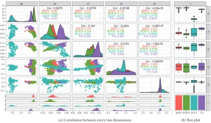
and flatten these 2D images into one dimension. In order to show the separability of these data, we perform covariance operations on them in order to establish correlations between two-dimensional features. Figure 5 shows the correlation and box plot of the first 5-dimensional features. Figure 5(a) is the correlation of two dimension features, and Figure 5(b) is the corresponding box plot. In Figure 5(a), the lower left corner part is the scatter plot of two-dimensional features, and the upper right part is the correlation coefficient

corre-sponding to the two-dimensional features.𝐶𝑜𝑟represents the

total correlation coefficient of the relevant two-dimensional features. Positive numbers indicate positive correlations and negative numbers indicate negative correlations. The greater the absolute value of these numbers, the more relevant the features of the corresponding two dimensions. From the

correlation coefficient, 𝐶𝑜𝑟’s absolute value is small which

shows that the correlation is low, indicating that they are independent of each other. From the scatter plot, we observe that they are very similar, which increases the difficulty of the recognition algorithm. In addition, from the box plot, there are abnormal points in the upper and lower bounds of the data. If these points are not removed in the learning set features, the performance of the algorithm will be affected.

50 X1 40

30 20 10 0 0.05 0.00

0.15 0.10 0.05 0.00

0.2 0.1 0.0

0.2

0.2 0.3 0.4 0.1

0.0

0.00 0.00 0.05 0.05 0.10 0.15 0.0 0.1 0.2 0.0 0.1 0.2

−0.05 −0.10

−0.05

−0.1

−0.1

−0.10 −0.05 −0.05 −0.1 −0.1

y

X2

X3

X4

X5

y

X1

BMP2

(a) Correlation between every two dimensions (b) Box plot

BTR70 SLICY T72

Figure 5: The correlation between the first 5-dimensional features after flattening SAR images of T72, BMP2, BTR70 and SLICY. (a)Correlation between every two dimensions and (b) box plot.

(1) Data Configuration of the SOC. Table 1 shows the data configuration of SOC. It contains two sets of data: data and test sets. The data set is used for the algorithm training. According to the label of the samples, the data set is divided into the labeled and unlabeled samples. The labeled samples, also known as the training set, have a number ranging from 3 to 40 per class. The unlabeled samples, also known as the learning set, have 190 samples per class. Regardless of the training or learning set, their target depression angle is

17∘. The testing set is used for algorithm testing. Its target

depression angle is 15∘. Regardless of data or test set, we use

the same variants of the targets, that is, T72 series sn 132 tanks, BMP2 series sn c21 armored vehicles, and BTR70 series sn c71 armored vehicles. We will verify the effectiveness

of the S2DP and IS2DP under these conditions in Section 4.1,

including their core components (LCI and WKFDA).

(2) Data Configuration of the EOC 1. Table 2 shows the data configuration of EOC 1. In Table 2, the training set is the same as that of Table 1. And the testing set is not the same version variants as the training set and the learning set. For example, the T72 is the sn s7 version in the test, but it is the sn 132 and sn 812 versions in the training and the learning sets, respectively. These conditions will help increase the recogni-tion difficulty of the algorithm. Other condirecogni-tions shown in Table 2, such as the number of data sets, the depression angle of data sets, and the depression angle of the test set, are the same as those shown in Table 1 and are not described here. We

will verify the generalization ability of the S2DP and IS2DP

under these conditions presented in Section 4.2.

(3) Data Configuration of the EOC 2. Table 3 shows the data configuration of EOC 2. It is formed by adding the interference target SLICY to the learning set of Table 2, further increasing the recognition difficulty of the algorithm. To highlight the advantages of the proposed algorithm, we

will compare the S2DP based IS2DP algorithm with the

semi-supervised depth learning method under EOC 2 in Section 4.3.

4.1. Effectiveness Evaluation Experiment

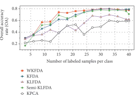
4.1.1. The Effectiveness of the WKFDA Feature Extraction. To verify the effectiveness of the WKFDA feature extraction, it is compared with the KFDA, kernel local linear dis-criminant analysis (KLFDA) [30], semi-supervised KLFDA (Semi-KLFDA) [31] and kernel principal component analysis (KPCA) [32]. After these algorithms have extracted features, they all use the standard SVM as the final classifier. The experimental data configuration is shown in Table 1, and with the change of the number of the labeled samples, the overall accuracy rates (OA) of different methods are obtained, as shown in Figure 6. The horizontal axis represents the number of each type of target labeled samples corresponding to different experiments and the vertical axis represents the overall accuracy rate.

Table 1: Data configuration of the SOC.

Data set

Testing set Training set (Labeled samples) Learning set (Unlabeled samples)

Target T72 BMP2 BTR70 T72 BMP2 BTR70 T72 BMP2 BTR70

Type sn 132 sn c21 sn c71 sn 132 sn c21 sn c71 sn 132 sn c21 sn c71

Quantity 3∼40 3∼40 3∼40 190 190 190 196 195 196

Depression 17∘ 17∘ 15∘

Table 2: Data configuration of the EOC 1.

Data set

Testing set Training set (Labeled samples) Learning set (Unlabeled samples)

Target T72 BMP2 BTR70 T72 BMP2 BTR70 T72 BMP2 BTR70

Type sn 132 sn c21 sn c71 sn 812 sn 9566 sn c71 sn s7 sn 9563 sn c71

Quantity 3∼40 3∼40 3∼40 190 190 190 196 195 196

Depression 17∘ 17∘ 15∘

Table 3: Data configuration of the EOC 2.

Data set

Testing set Training set (Labeled samples) Learning set (Unlabeled samples)

Target T72 BMP2 BTR70 T72 BMP2 BTR70 SLICY T72 BMP2 BTR70

Type sn 132 sn c21 sn c71 sn 812 sn 9566 sn c71 — sn s7 sn 9563 sn c71

Quantity 3∼40 3∼40 3∼40 190 190 190 190 196 195 196

Depression 17∘ 17∘ 15∘

WKFDA

KLFDA Semi-KLFDA KPCA

ra

te (O

A)

O

veral

l acc

urac

y

0.2 0.4 0.6 0.8

Number of labeled samples per class 5 10 15 20 25 30 35 40

KFDA

Figure 6: The OA trend chart of different feature extraction algorithms with the number of labeled samples changes in SOC experiment. Here, these feature extraction algorithms use SVM as classifier.

24, the WKFDA’s classification results are better than the KFDA. When the number of the labeled samples is greater than 24, their classification results are almost the same. It shows that KFDA and WKFDA have good feature extraction capabilities, while the WKFDA is suitable for dealing with a small quantities of labeled samples. For the KFDA and Semi-KLFDA, when the number of the labeled samples is less than 20, the Semi-KLFDA’s classification results are better than the KFDA. When the number of labeled samples is greater than

20, their classification results are almost the same. For the KPCA, as the number of the labeled samples increases, its classification results are always poor.

In order to understand the above experimental results, we take a close look at the projections of the learning samples under the condition that the same number of the labeled samples is taken. Figures 7(a), 7(b), 7(c), 7(d), and 7(e) shows the projection of the learning set for KPCA, KLFDA, Semi-KLFDA, KFDA, and WKFDA algorithms respectively when the number of the labeled samples is 20. As can be seen from Figure 7, the projection result shown in (e) is the best, where we can classify the three targets, second best is (d) and then (c), (b), and (a). The quality of the projection results mainly depends on whether or not the feature extraction algorithm can effectively extract features from the SAR images.

For the KPCA algorithm, it only reduces the original features of the SAR images. As the number of the labeled samples increases, the classification accuracy of the KPCA features continues to increase. The original features of the SAR images are difficult to identify. Therefore, the classifica-tion accuracy of SVM based on the KPCA features is poor, shown in Figure 7(a).

BMP2 BTR70 T72

(a)

BMP2 BTR70 T72

(b)

BMP2 BTR70 T72

(c)

BMP2 BTR70 T72

(d)

BMP2 BTR70 T72

(e)

Figure 7: The projections of the learning set for KLFDA, Semi-KLFDA, and KPCA, respectively, when the number of the labeled samples is 20. (a)KPCA; (b)KLFDA; (c)Semi-KLFDA; (d)KFDA; (e)WKFDA.

resulting in more confusing clutters in the projection space. This is observed from Figures 7(b) and 7(c).

For the KFDA and WKFDA algorithms, both of them well use the difference between different classes and the sim-ilarities in the same classes. Therefore, the projections shown in Figures 7(d) and 7(e) are better than those of the other methods. We know that the KFDA and WKFDA algorithms are supervised algorithms which guide the projection of the unlabeled sample features based on the features of the labeled samples. Therefore, whether or not these algorithms are good at learning the labeled sample features will affect the quality of the projection of the unlabeled sample features. In the process of the labeled sample feature learning, the KFDA algorithm forces the interclass samples to be as far apart as possible in addition to forcing the samples intraclasses to be as close as possible. At the same time, it may cause the algorithm to overfit and is difficult to guide the unlabeled sample features to be projected onto the optimal direction. The WKFDA algorithm is able to give the samples different weights so that the intraclass samples are close to each other with a certain weight. This can balance the concentration characteristics of the samples (the intraclass samples aggregate with each other and have a certain spatial structure) and can fully utilise the spectral information of the samples and reduces the algorithm’s overfitting. Therefore, the results shown in Figure 7(e) seem better than those of Figure 7(d).

To further explore the impact of weighting on the WKFDA algorithm, taking the same labeled samples, Figure 8 shows the results of the KFDA and WKFDA algorithms for learning the features of the labeled samples. Figure 8(a) shows the KFDA features. Although the interclass distance is significant, the intraclass samples are concentrated, almost grouping to a point, which is easy to cause overfitting of the algorithm. Figure 8(b) shows the WKFDA features. Under the condition that the interclasses is separable, the intraclass distance is relatively large, which is easy to learn the sample information and suppress the overfitting of the algorithm. Here, Figure 8(b) also shows that different weights can result in different intraclass distance. Compared with the weight of 100, the intraclass sample space is larger when the weight is 50, and the interclasses can be well spaced, which makes it easier to learn sample information.

4.1.2. The Effectiveness of the LCI for Labeling Unlabeled Samples. To verify the effectiveness of the LCI for label-ing unlabeled samples, uslabel-ing the WKFDA features of the Section 4.1.1 experiments, LCI is compared with the SVM and

S3VM classifiers under the DP clustering conditions. Using

BMP2 BTR70 T72

(a)

Weight=200

Weight=200

Weight=50

Weight=50

BMP2 BTR70 T72

Weight=200 Weight=50

(b)

Figure 8: The projection of the KFDA and WKFDA with the same number of the labeled samples. (a)KFDA and (b)WKFDA.

shown in Figure 9. The horizontal axis represents the number of each type of the labeled target samples corresponding to different experiments, and the vertical axis represents the overall accuracy rate. As can be seen from Figure 9, the

accuracy of LCI and S3VM is better than SVM. With more

and more labeled samples, the accuracy of LCI and S3VM is

almost the same.

We know that the SVM, as a supervised learning method, requires a large number of labeled samples. Because the DP algorithm cannot provide enough labeled samples for the

SVM, the SVM classification results are poor. For S3VM and

LCI, as a semi-supervised method, when the DP clustering

LCI

SVM

ra

te (O

A)

O

veral

l acc

urac

y

0.4 0.6 0.8 1.0

Number of labeled samples per class 5 10 15 20 25 30 35 40

３3_VM

Figure 9: The OA trend chart of the LCI, S3VM, and SVM algorithms as the number of labeled samples changes in the SOC experiment.

(a)

Cluster Core Cluster Halo Error Point

(b)

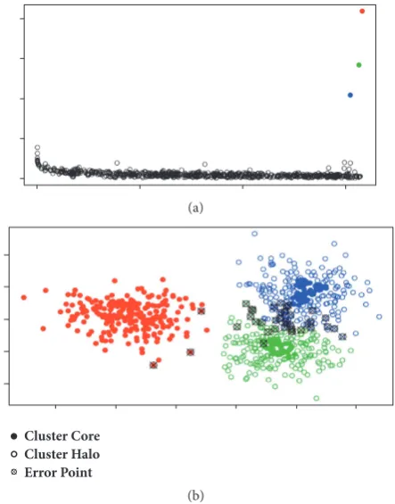
Figure 10: The clustering results of DP on the learning set when the number of the labeled samples is 21. (a) Red circle, green circle, and blue circle are the cluster centers selected by the DP; (b)the clustering results of the DP.∙are the cluster cores,∘are clustered halos, and⊗ are clustering error samples.

outcome is reliable, they collect enough labeled samples to improve the recognition performance. Figure 10 shows the clustering results of the DP on the learning set when the number of the labeled samples is 21. In Figure 10(a), red circle, green circle, and blue circle are the cluster centers selected by the DP. The DP algorithm recommends that the learning set be divided into 3 categories, which is consistent with the actual situation. Figure 10(b) shows the clustering results of

Semi-supervised Fanny Semi-supervised Clara

O

veral

l acc

urac

y ra

te (O

A)

0.4 0.5 0.6 0.7 0.8 0.9 1.0

Number of labeled samples per class

5 10 15 20 25 30 35 40

３2DP

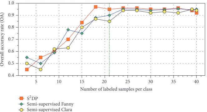
Figure 11: The OA trend chart of the S2DP, semi-supervised Clara, and semi-supervised Fanny with the number of labeled samples changes in SOC experiment.

are clustering errors. From Figure 10(b), the DP clustering has only minor errors and the result is quite accurate, further

demonstrating that the recognition accuracy of the S3VM and

LCI is equivalent. In addition, these errors are located in the cluster halos. In the LCI algorithm, the cluster halos and the cross-clustering samples will be deleted to ensure that the final labeled samples are reliable. Therefore, compared to the

S3VM, the LCI recognition results are more consistent.

4.1.3. Verifying the Recognition Performance of 𝑆2𝐷𝑃. In

order to verify the recognition performance of S2DP, S2DP

is compared with its similar semi-supervised methods. These similar semi-supervised methods are the semi-supervised

algorithms that replace DP in S2DP with other classical

clus-tering algorithms: Clara [25] and Fanny [26], namely, semi-supervised Clara and semi-semi-supervised Fanny. The experi-mental data configuration is shown in Table 1. With the changing numbers of the labeled samples, the OA trend chart of three methods is obtained, as shown in Figure 11. The horizontal axis represents the number of each type of labeled target samples corresponding to different experiments, and the vertical axis represents the overall accuracy rate.

By comparing the S2DP with the semi-supervised Clara

and semi-supervised Fanny, the classification results of the different methods are greatly influenced by the number of the labeled samples. When the number of the labeled samples is less than 24, the overall accuracy of the three methods is continuously improved with the increase of the labeled

samples. For the curve smoothness, the curve of the S2DP

looks consistent over the curves of the other two methods. When the number of the labeled samples reaches 15, the

recognition accuracy of S2DP is higher than that of the

other two methods. When the number of the labeled samples reaches 24, the three methods have the same recognition

accuracy and the curve trend is stable, but the S2DP is still

better than the other two methods. Therefore, the S2DP is

superior to the other two algorithms in terms of stability and classification accuracy.

When the labeled samples are very few, the DP clustering

results of S2DP are too divergent to represent the unlabeled

samples. Only few labeled samples are generated from the cluster core samples. In the end, the classification accuracy

of the S2DP will not be high. As the number of the labeled

samples increases, more and more labeled samples are gen-erated by the cluster cores, which are also quite reliable. The

S2DP classification accuracy is greatly improved. The other

two methods are similar. However, as the number of the labeled samples increases, it is difficult for semi-supervised Clara and semi-supervised Fanny to guarantee the reliability of the labeled samples from the unlabeled samples during the clustering process. Therefore, their stability is not as good as

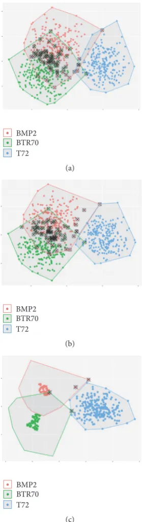
that of S2DP. Figure 12 shows the three algorithms generate

labeled samples from the learning set when the number of the

labeled samples is 21.⊗are clustering errors. Obviously, the

labeled samples generated by the S2DP algorithm are more

reliable than the other two methods.

The Sections 4.1.1–4.1.3 experimental results show the relationship between the number of the labeled samples and

the S2DP, verifying the validity of the WKFDA, LCI, and

DP as the key step in the S2DP. It shows that the S2DP,

compared with the other two methods, can achieve the best classification result when the initial labeled samples reach a certain number. But when the labeled samples are too few, its classification precision decreases. Therefore, the ability of the

modified IS2DP to query semi-supervised samples needs to

be verified.

4.1.4. Verifying the 𝐼𝑆2𝐷𝑃 in Ability to Query the Semi-Labeled Samples. When the labeled samples are few, the

IS2DP can select the semi-labeled samples from the unlabeled

samples as the labeled samples. In the Section 1, we know that

PS3VM-D is also a semi-supervised method, which considers

reliable incremental samples as semi-supervised samples

by sample similarity. Therefore, PS3VM-D is selected as a

BMP2 BTR70 T72

(a)

BMP2 BTR70 T72

(b)

BMP2 BTR70 T72

(c)

Figure 12: The semi-supervised Clara, semi-supervised Fanny, and S2DP generate reliable labeled samples from the learning set when the number of the labeled samples is 21.⊗are clustering errors. (a) The Clara clustering results; (b) the Fanny clustering results; (c) the DP cluster cores.

configuration is shown in Table 1. With the change of the number of the labeled samples, the OA trend chart of two methods is obtained, as shown in Figure 13. The horizontal axis represents the number of each type of the labeled target samples corresponding to different experiments and the vertical axis represents the overall accuracy rate.

When the number of the labeled samples is less than 25,

the classification accuracy of PS3VM-D is obviously lower

than that of IS2DP, indicating that IS2DP is more suitable for

the case of too few labeled samples. When the number of the

labeled samples is more than 25, the IS2DP and PS3VM-D

have the same accuracy. It shows that the PS3VM-D also gets

enough labeled sample information, and the classification accuracy is improved.

We know that the core of PS3VM-D is SVM. The optimal

classification surface of PS3VM-D is mainly influenced by

SVM. The PS3VM-D relies heavily on the labeled samples.

It needs enough quantity to obtain a universal classification surface. Therefore, its classification performance varies sig-nificantly with the number of labeled samples and cannot remain stable until the labeled samples are sufficient. The

classification performance of the IS2DP is largely determined

by the DP and WKFDA, which makes the IS2DP more stable

and accurate when the labeled samples are very few due to the sample description ability of the DP and the effective use of the labeled samples by the WKFDA.

4.2. Evaluation of Generalization Ability. The following will

verify the generalization capabilities of S2DP and IS2DP

under the EOC 1.

4.2.1. Verifying the𝑆2𝐷𝑃Generalization Capabilities. In

Sec-tion 4.1.2, the comparison between LCI and S3VM algorithm

is actually the comparison of S2DP with S3VM based on

WKFDA and DP (WKFDA+DP+S3VM). The recognition

accuracy of S2DP and WKFDA+DP+S3VM is equivalent

in the SOC experiments. Here, we continue to compare

the S2DP and WKFDA+DP+S3VM. The experimental data

configuration is shown in Table 2. With the change of the number of labeled samples, the OA trend chart of two methods is obtained, as shown in Figure 14. The horizontal axis represents the number of each type of the labeled target samples corresponding to different experiments, and the vertical axis represents the overall accuracy rate.

In Figure 14, the recognition accuracy of S2DP and

WKFDA+DP+S3VM algorithms increases with the

increas-ing number of the labeled samples, and their final accuracy

is equivalent. However, the curve of the S2DP is relatively

smooth. This shows that our method is stable and robust. To verify this conclusion, we perform visual analysis of the key steps of the two methods, when the number of samples is 21. Figure 15(a) shows the features of the training

and learning sets after the WKFDA processing.∙represents

the learning samples and ∗ represents the initial labeled

sample. Figure 15(b) is the actual classification map of the

WKFDA features after the DP clustering has been achieved.∙

represents the clustering core and∘represents the clustering

halo. Figure 15(c) is the true classification map of Figure 15(b).

∙represents the clustering core, ⊗represents the clustering

error sample, and?represents the sample of the next step

O

veral

l acc

urac

y ra

te (O

A)

0.5 0.6 0.7 0.8 0.9 1.0

Number of labeled samples per class

5 10 15 20 25 30 35 40

I３2DP P３3VM-D

Figure 13: The OA trend chart of the IS2DP and PS3VM-D as the number of the labeled samples changes in the SOC experiment.

O

veral

l acc

urac

y ra

te (O

A)

0.4 0.6 0.8 1.0

Number of labeled samples per class

5 10 15 20 25 30 35 40

３2_DP

WKFDA+DP+３3VM

Figure 14: The OA trend chart of the S2DP and WKFDA+DP+S3VM as the number of labeled samples changes in the EOC 1 experiment.

samples are not cleared. As can be seen from Figure 15(b), the DP algorithm divides the WKFDA features into 5 clusters. Among these 5 clusters, clusters 1 and 3 have cluster haloes, and clusters 2, 4, and 5 are all clustered cores. As can be seen

from Figure 15(c), the initial labeled samples (∗samples) are

not included in clusters 4 and 5 and, therefore, the samples of clusters 4 and 5 need to wait for the next step of the algorithm to identify and label. Clusters 1, 2, and 3 contain initial labeled

samples (∗samples), so they get the same label as the initial

labeled sample. In the clustering halos of clusters 1 and 3, there

are many clustering error samples (⊗samples) caused by the

confused samples shown in Figure 15(a). This means that, in the future, they will affect the performance of the recognition

algorithm if these⊗samples are not cleared.

For the WKFDA+DP+S3VM algorithm, in the S3VM

training process, for one thing, the S3VM cannot clear the⊗

samples in Figure 15(c). And for another, for the?samples in

Figure 15(c), the S3VM can only identify them by traversing

the samples. Therefore, the WKFDA+DP+S3VM algorithm

is unstable and inefficient. For the S2DP algorithm, once the

features of Figure 15(c) are input into the LCI, the LCI algo-rithm removes the unreliable features such as the clustering halos and cross-clustering features and makes full use of the cluster cores as reliable samples. Once the labeled samples are included in the cluster core, the other unlabeled samples are labeled with the labels of the labeled samples. For cluster cores that do not contain labeled samples, only the clustering center is identified, and the label of the whole cluster core can be obtained, which greatly improves the recognition efficiency. Figure 16 is a sequence diagram showing the recognition of the DP clustering result of Figure 15(b) by the LCI in the

S2DP algorithm. Figure 16(a) is the visualization of the DP

clustering results after removing the interference samples. Figure 16(b) is the result diagram of LCI’s final recognition of the DP clustering. As can be seen from Figure 16(a), both

the confusing sample in Figure 15(a) and the ⊗ sample in

BMP2 BTR70 T72

(a)

(b)

BMP2 BTR70 T72

(c)

Figure 15: In EOC 1 experiment, the visualization results of the first two steps of the S2DP and WKFDA+DP+S3VM algorithms when the number of the samples is 21. (a) WKFDA features:∙represents the learning set and∗represents the initial labeled samples; (b) actual classification map of WKFDA features after DP clustering has been carried:∙represents the clustering core and∘represents the clustering halo; (c) true classification map of (b):∙represents the clustering core,⊗represents the clustering error sample, and ? represents the sample of the next step of the algorithm to be identified.

expanded labeled samples. Thus, S2DP is quite reliable. In this

way, the above conclusions are verified.

4.2.2. Verifying the 𝐼𝑆2𝐷𝑃 Generalization Capabilities. In

Section 4.2.1, the S2DP is relatively stable, but its recognition

accuracy is relatively low when the number of the labeled

samples is less than 21. Therefore, the IS2DP is required to

generate a large number of the labeled samples to improve

BMP2 BTR70 T72

(a)

BMP2 BTR70 T72

(b)

Figure 16: The sequence diagram of the LCI algorithm for identi-fying DP clustering results in Figure 15(b). (a) Visualization of DP clustering results after removing the interference samples; (b) LCI’s final recognition visualization of DP clustering.∙ represents the clustering core;∗represents the initial labeled sample;?represents the sample of the next step of the algorithm to be identified;⊗ represents the sample for labeling errors.

the recognition accuracy of S2DP. Here, we compare the

IS2DP+S2DP and S2DP. The experimental data configuration

is shown in Table 2 with the change of the number of the labeled samples, and the OA trend chart of the two methods is obtained, as shown in Figure 17. The horizontal axis represents the number of each type of target labeled samples corresponding to different experiments; the vertical axis represents the overall accuracy rate.

From Figure 17, we can see that when the number of the labeled samples is less than 21, the recognition performance

of IS2DP+S2DP is 10% higher than that of S2DP. With the

number of labeled samples larger than 21, their classification accuracy is equivalent. To verify this conclusion, we apply 100

iterations onto IS2DP when the number of labeled samples

is 15. The labeled samples generated by IS2DP are counted,

O

veral

l acc

urac

y ra

te (O

A)

0.4 0.6 0.8 1.0

Number of labeled samples per class

5 10 15 20 25 30 35 40

I３2DP+３2DP

３2_DP

Figure 17: The OA trend charts of the IS2DP+S2DP and S2DP with the number of labeled samples changes in EOC 1 experiment.

Ladder Network Temporal Ensembling

O

veral

l acc

urac

y ra

te (O

A)

0.5 0.6 0.7 0.8 0.9

Number of labeled samples per class

5 10 15 20 25 30 35 40

I_３2DP+_３2DP

Figure 18: The OA trend charts of the IS2DP+S2DP, Ladder Network, and Temporal Ensembling with the number of labeled samples changes in EOC 2 experiment.

4.3. Comparison with Semi-Supervised Deep Learning. The semi-supervised deep learning algorithms, Ladder Network [7] and Temporal Ensembling [8], which contain a supervised and unsupervised learning process, similar to our algorithm. Therefore, we choose these two methods to compare with the

IS2DP-based S2DP algorithm (IS2DP+S2DP). In addition to

using SAR images as experimental data, we also use a set of publicly available optical image data to verify the effectiveness of our algorithm.

4.3.1. Testing with SAR Images. The experimental data con-figuration is shown in Table 3, and with the change of the number of the labeled samples, the OA trend chart of three methods is obtained, as shown in Figure 18. The horizontal axis represents the number of each type of labeled target samples corresponding to different experiments, and the vertical axis represents the overall accuracy rate.

In Figure 18, the recognition accuracy of the three meth-ods is increasing with the increase of the labeled samples. From the curve smoothing, the accuracy curves of the Ladder

Network and the Temporal Ensembling are fluctuating, especially the Temporal Ensembling. Comparing them, the

accuracy curve of the IS2DP+S2DP is relatively consistent.

From the classification accuracy, when the number of the labeled samples is less than 33, the results obtained by Ladder Network and Temporal Ensembling are not much

different, but significantly lower than that of IS2DP+S2DP.

When the number of the labeled samples reaches 33, the

classification accuracy of IS2DP+S2DP is slightly better than

that of Ladder Network. These results indicate that the learning set containing the interference samples has a great influence on the recognition performance of the Ladder Network and Temporal Ensembling. Because the Ladder Network and Temporal Ensembling were unable to remove these interference samples during the training process, their recognition accuracy was unstable and not high. Different

from them, the IS2DP+S2DP can select reliable unlabeled

Table 4: The IS2DP generates labeled samples from the learning set when the number of labeled samples is 15 in EOC 1 experiment.

Target Learning set Generate labeled samples Reject Accuracy of each type of target(%)

Correct Error

T72 190 167 11 12 87.89

BMP2 190 163 13 14 85.79

BTR70 190 172 8 10 90.53

Overall accuracy 88.07

Table 5: Under EOC 2, when labeled samples number 21, recognition results (confusion matrix) of the learning set by trained Temporal Ensembling.

T72 BMP2 BTR70 Accuracy of each type of target(%)

T72 65 3 122 34.21

BMP2 0 174 16 91.58

BTR70 0 0 190 100

SLICY 0 0 190 0

Overall accuracy 56.45

to 21, we will analyze the use of the learning set by the three methods below.

In the Temporal Ensembling algorithm, one neutral network conducts two different works, supervised learning and unsupervised learning. Figures 19(a)–19(c), respectively, show losses in these two processes and in the whole method. Observed from the curve fluctuation, supervised learning loss in Figure 19(a) is the most stable while unsupervised learning in Figure 19(b) fluctuates significantly. It demon-strates that neural network performs well in learning labeled samples, but is still unstable to handle the learning set, thus resulting in unstable overall loss as shown in Figure 19(c). Finally, the Temporal Ensembling algorithm utilizes the learning set by 56.45% only, which is calculated based on the trained neutral network’s recognition of the learning set. Recognition results of the learning set by the Temporal Ensembling algorithm is displayed in Table 5 (confusion matrix). Observed from the confusion matrix, the remaining 43.55% disturbs the learning process, for instance, by misrec-ognizing SLICY as BTR70 targets.

Similar to temporal ensembling algorithm, the neu-tral network in the Ladder Network algorithm consists of supervised learning and unsupervised learning as well. Figures 20(a)–20(c), respectively, show losses in these two processes and by the whole method. Observed from the curve fluctuation shown in Figure 20(a), supervised learning loss significantly fluctuates, probably because of inadequate labeled samples; in Figure 20(b), unsupervised learning per-forms stably, probably resulting from unsupervised learning (Autoencoder) embedded in the Ladder Network algorithm which could learn and recognize unlabeled samples and reduce certain interference. Thus, the overall loss shown in Figure 20(c) performs stably. Therefore, comparing with tem-poral ensembling, Ladder Network improves the utilization of the learning set to 68.42% (as shown in Table 6 confusion matrix), enhancing its recognition performance as well.

Differing from temporal ensembling and ladder network,

the IS2DP+S2DP algorithm identifies reliable unlabeled

sam-ples by iterations before implementing feature learning, instead of directly learning features from the unlabeled

samples. Here we employ 300 iterations on the IS2DP+S2DP

algorithm for fair comparison. Figures 21(a)–21(c) show the screening of the reliable samples in the learning set during one iteration: (a) projection of the WKFDA algorithm on the learning set; (b) DP clustering result; (c) reliable samples labeled by LCI. In Figure 21, red circle, green circle, light blue circle, and blue circle represent BMP2, BTR70, T72,

and SLICY target samples, respectively, and∗represents the

labeled samples. Confused by SLICY interference targets, the WKFDA algorithm has some issue in projecting the learning set but performs well in dividing different samples during the DP clustering, and successfully identify SLICY during

the LCI labeling process. Finally, IS2DP+S2DP improves the

utilization of the learning set to 82.76% (as shown in Table 7). As 28.95% unreliable sample rejecting recognition will be deleted, only 10% false samples affects the performance; thus

IS2DP+S2DP’s recognition performance can be improved.

4.3.2. Testing with Optical Images. To verify the effectiveness of the proposed method on other data sets, we use optical

image data to test IS2DP+S2DP. These optical image data

come from some publicly available databases, and the detailed data configuration is shown in Table 8. The images of cats and dogs are from the database of the Kaggle competition platform [33]; the images of panda are from the ImageNet database [34]; the images of airplanes, motorbike, and faces are from the caltech101 database [35].

Table 6: Under EOC 2, when the labeled samples’ number is 21, the recognition results (confusion matrix) of the learning set by the trained ladder network.

T72 BMP2 BTR70 Accuracy of each type of target(%)

T72 166 10 4 87.37

BMP2 12 178 0 93.68

BTR70 2 12 176 92.63

SLICY 67 53 70 0

Overall accuracy 68.42

Table 7: Under EOC 2, when labeled samples number 21, recognition results of the learning set by IS2DP+S2DP after 300 iterations.

Target Learning set Generate labeled samples Reject Accuracy of each type of target(%)

Correct Error

T72 190 155 12 23 81.58

BMP2 190 162 17 11 85.26

BTR70 190 147 22 21 77.37

SLICY 190 — 25 165 86.84

Overall accuracy 82.76

(a)

(b)

(c)

Figure 19: Under EOC 2, when labeled samples number 21, Tempo-ral Ensembling losses during training: (a) supervised learning loss; (b)unsupervised learning loss; (c) overall loss.

(a)

(b)

(c)

BMP2

BTR70

T72

SLICY

(a)

BMP2

BTR70

T72

SLICY

(b)

BMP2

BTR70

T72

SLICY

(c)

Figure 21: Under EOC 2, when the labeled samples number is 21, IS2DP+S2DP’s outcomes of the learning set: (a) WKFDA’s projection of the learning set; (b) DP clustering result; (c) reliable samples selected and labeled by LCI. Red circle, green circle, light blue, and blue circle represent BMP2, BTR70, T72, and SLICY target samples, respectively, and∗represents labeled sample.

but also other 3 types of interference targets (airplanes, motorbike, and faces) with the same number of unlabeled interested targets. Under such conditions, the Ladder

Net-work, Temporal Ensembling, and IS2DP+S2DP are tested and

compared. With the change of the number of the labeled samples, the OA trend chart of three methods is obtained,

as shown in Figure 22. The horizontal axis represents the number of each type of target labeled samples corresponding to different experiments; the vertical axis represents the overall accuracy rate.

In Figure 22, the identification accuracy of our method