City, University of London Institutional Repository
Citation
:
Cox, A., De Visscher, M. and Martin, P. (2009). The blocks of the Brauer algebra
in characteristic zero. Representation Theory, 13, pp. 272-308. doi:
10.1090/S1088-4165-09-00305-7
This is the unspecified version of the paper.
This version of the publication may differ from the final published
version.
Permanent repository link:
http://openaccess.city.ac.uk/372/
Link to published version
:
http://dx.doi.org/10.1090/S1088-4165-09-00305-7
Copyright and reuse:
City Research Online aims to make research
outputs of City, University of London available to a wider audience.
Copyright and Moral Rights remain with the author(s) and/or copyright
holders. URLs from City Research Online may be freely distributed and
linked to.
Volume 00, Pages 000–000 (Xxxx XX, XXXX) S 1088-4165(XX)0000-0
THE BLOCKS OF THE BRAUER ALGEBRA IN CHARACTERISTIC ZERO
ANTON COX, MAUD DE VISSCHER, AND PAUL MARTIN
Abstract. We determine the blocks of the Brauer algebra in characteristic zero. We also give information on the submodule structure of standard mod-ules for this algebra.
1. Introduction
The Brauer algebraBn(δ) was introduced in [Bra37] in the study of the
represen-tation theory of orthogonal and symplectic groups. OverC, and for integral values
ofδ, its action on tensor spaceT = (C|δ|)⊗n can be identified with the centraliser
algebra for the corresponding group action. This generalises the Schur-Weyl duality between symmetric and general linear groups [Wey46].
Ifnis fixed, then for allδ≥nthe centraliser algebra EndO(δ)(T) has multimatrix
structureindependentofδ, and Brauer’s algebraBn(δ) unifies these algebras, having
a basis independent ofδ, and a law of composition which makes sense over any field
k and for any δ∈k. The Brauer algebra is well defined in particular for positive integralδ < n, but the action onT is faithful for positive integralδ if and only if
δ≥n.
In classical invariant theory one is interested in the Brauer algebraper seonly in so far as it coincides with the centraliser of the classical group action onT; i.e., in the case ofδintegral with|δ| large compared ton. Here we take another view, and consider the stable properties for fixedδ and arbitrarily largen. In such cases
Bn(δ) is not semisimple for δ integral. However it belongs to a remarkable family
of algebras arising both in invariant theory and in statistical mechanics for which this view is very natural. (For example when considered from the point of view of transfer matrix algebras in statistical mechanics [Mar91].) Indeed much of the structure ofBn(δ) can be recovered from a suitable global limit ofnby localisation
(and in this sense its structure does not depend onn).
2000Mathematics Subject Classification. Primary 20G05.
c
1997 American Mathematical Society
This family of algebras can be introduced as follows. Consider the diagram of commuting actions onT, with|δ|=N:
GL(N)
> > > > > > > > > >
CΣn
∪ ∩
O(N) //T oo Bn(N)
∪ ∩
ΣN
@
@
Pn(N)
^
^
== ==
== ==
==
where the actions of the algebra on the right centralise the action of the group on the left in the same row, and vice versa. The bottom row consists of the diagonal action of ΣN permuting the standard ordered basis of CN on the left, and the
partition algebraPn(N) on the right. The partition algebraPn(δ) (for anyδ) has a
basis of partitions of two rows ofnvertices. The Brauer algebra is the subalgebra with basis the subset of pair partitions, andCΣn is the subalgebra with basis the
pair partitions such that each pair contains a vertex from each row. The Brauer algebra also has a subalgebra with basis the set of pair partitions which can be represented by noncrossing lines drawn vertex-to-vertex in an interval of the plane with the rows of vertices on its boundary. This is the Temperley-Lieb algebraTn(δ).
All of these algebras are rather well understood overC, with the exception ofBn.
All their decomposition matrices are known, and all of their blocks can be described by an appropriate geometric linkage principle. For Σn both data are trivial, since
CΣnis semisimple. ForTneach standard module has either one or two composition
factors and its alcove geometry is affineA1 (affine reflections on the real line). For
Pn each standard module has either one or two composition factors and its alcove
geometry is affineA∞ (although locally the block structure looks like affineA1).
OverC, the Brauer algebra is semisimple forδsufficiently large, and is generically
semisimple [Bro55]. Hanlon and Wales studied these algebras in a series of papers [HW89b, HW89a, HW90, HW94] and conjectured thatBn(δ) is semi-simple for all
non-integral choices ofδ. This was proved by Wenzl [Wen88].
In this paper we determine the blocks ofBnforδintegral. The simple modules of
Bn may be indexed by partitions of those natural numbers congruent tonmodulo
2 and not exceeding n, and hence by Young diagrams (if δ = 0 then the empty partition is omitted). We will call these indexing objectsweights. Given δ∈R a ring we can associate achargech(ǫ)∈Rto each boxǫin a Young diagram, as shown in Figure 1. We will also refer later to the usualcontentof boxes which, for the box
ǫin rowiand columnj isc(ǫ) =j−i. It is easy to see thatch(ǫ) =δ−1 + 2c(ǫ). For each pair of diagramsλandµwe will also need to consider the skew partitions
λ/(λ∩µ) andµ/(λ∩µ) consisting of those boxes occurring inλbut notµand in
µbut notλ.
With these notations we can now state the two main results of the paper (which are valid without restriction onδ).
δ−1 δ+ 1 δ+ 3 · · ·
δ−3 δ−1 δ+ 1 · · ·
δ−5 δ−3 δ−1 · · ·
[image:4.595.246.367.120.225.2].. . ...
Figure 1. The charges associated to boxes in a Young diagram
(i) The boxes in λ/(λ∩µ)(respectively µ/(λ∩µ)) can be put into pairs whose charges sum to zero;
(ii) ifλ/(λ∩µ)(respectivelyµ/(λ∩µ)contains −1
1 with no 1 to the right of these boxes then it contains an even number of 1/-1 pairs.
Examples illustrating this result are given in Example 4.9.
Theorem 7.3 (Summary). For any integral δ and natural number l a standard module can be constructed (for some Bn(δ)) whose socle series length is greater
thanl. This module also has a socle layer containing at least l simples.
The second result shows that the structure of standard modules can become arbitrarily complicated. This is in marked contrast to the partition and Temperley-Lieb algebra, and symmetric group, cases.
To prove these results we use the theory of towers of recollement developed in [CMPX06]. This approach is already closely modelled, for Bn, in work of Doran,
Wales, and Hanlon [DWH99] (since both papers use the methods developed in [Mar96]). This key paper of Doran, Wales and Hanlon will be the starting point for our work, and we will generalise and refine several of their results.
The ‘diagram’ algebrasPn⊃Bn⊃Tnare amenable to many powerful
represen-tation theory techniques, and yet the represenrepresen-tation theory of the Brauer algebra is highly non-trivial in comparison to the others. We shall see that, in terms of degree of difficulty, the study of Brauer representation theory in characteristic zero is an intermediate between the study of ‘classical’ objects in characteristic zero and the grand theme of the representation theory of finite dimensional algebras, the study of Σn in characteristicp.
Another such intermediate class of objects are the Hecke algebras of typeA at roots of unity, which are Ringel dual to the generalised Lie objects known as quan-tum groups. The Brauer algebraBn in characteristic zero has, through its global
limit, more Lie-theory-like structure than Σnin characteristicp(for which not even
The paper begins with a section defining the various objects of interest, and a review of their basic properties in the spirit of [CMPX06]. This is followed by a brief section describing some basic results about Littlewood-Richardson coefficients which will be needed in what follows. In Section 4 we begin the analysis of blocks by giving a necessary condition for two weights to be in the same block. This is based on an analysis of the action of certain central elements in the algebra on standard modules, and inductive arguments using Frobenius reciprocity. Section 5 constructs homomorphisms between standard modules in certain special cases, generalising a result in [DWH99]. Although not necessary for the main block result, this is of independent interest.
The classification of blocks is completed in Section 6. The main idea is to show that every block contains a unique minimal weight, and that there is a homo-morphism from any standard labelled by a non-minimal weight to one labelled by a smaller weight. We also describe precisely which weights are minimal in their blocks.
In Section 7 we consider certain explicit choice of weights, and show inductively, via Frobenius reciprocity arguments, that the corresponding standards can have arbitrarily complicated submodule structures. We conclude by outlining the mod-ifications to our arguments required in the caseδ= 0.
The structure of the Brauer algebra becomes much more complicated when con-sidered over an arbitrary fieldk. For generalkandδintegral this algebra still acts as a centraliser algebra; this has been shown in a recent series of papers for the symplectic case [Dot98, Oeh01, DDH08], and in odd characteristic for the orthogo-nal case [DH]. A necessary and sufficient condition for semisimplicity (which holds over arbitrary fields) was given recently by Rui [Rui05]. The study of Young and permutation modules for these algebras has been started in [HP06].
Since this paper was submitted we have founded a reformulation of our block result in terms of an alcove geometry of typeD [CDM]. This has inspired a new proof of the block result using symplectic Schur functors by Donkin and Tange [DT].
2. Preliminaries
In this section we will consider the Brauer algebra defined over a general fieldk
of characteristicp≥0, although we will later restrict attention to the casek=C.
After reviewing the definition of the Brauer algebra, we will show that families of such algebras form towers of recollement in the sense of [CMPX06] (which we will see follows from various results of Doran et. al. [DWH99]). This will be the framework in which we base our analysis of these algebras.
Given n∈N and δ∈k, theBrauer algebra Bn(δ) is a finite dimensional
asso-ciative k-algebra generated by certain Brauer diagrams. A general (n, t)-(Brauer) diagramconsists of a rectangular box (orframe) withndistinguished points on the northern boundary andtdistinguished points on the southern boundary, which we callnodes. Each node is joined to precisely one other by a line, and there may also be one or more closed loops inside the frame. Those diagrams without closed loops are calledreduced. We will label the northern nodes from left to right by 1,2, . . . , n
will be called northern (respectively southern) arcs; those connecting a northern node to a southern node will be calledpropagating lines.
=
[image:6.595.134.478.146.206.2]x = δ
Figure 2. Multiplication of two diagrams inB6(δ)
Given an (n, t)-diagramAand a (t, u)-diagramB, we define the productAB to be the (n, u)-diagram obtained by concatenation ofAaboveB (where we identify the southern nodes ofAwith the northern nodes ofBand then ignore the section of the frame common to both diagrams). As a set, the Brauer algebraBn(δ) consists of
linear combinations of (n, n)-diagrams. This has an obvious additive structure, and multiplication is induced by concatenation. We also impose the relation that any non-reduced diagram containingmclosed loops equalsδmtimes the same diagram
with all closed loops removed. A basis is then given by the set of reduced diagrams. An example of a product of two diagrams in given in Figure 2. For convenience, we set B0(δ) =k. When no confusion is likely to arise, we denote the algebraBn(δ)
simply by Bn.
We will now apply as much as possible from the general setup of [CMPX06] to the Brauer algebra. The labels (A1), (A2), etc., refer to the axioms in that paper. Henceforth, we assume that δ6= 0; for the caseδ= 0 see Section 8.
For n ≥2 consider the idempotent en in Bn defined by 1/δ times the Brauer
diagram whereiis joined to ¯ifori= 1, . . . n−2, andn−1 is joined tonandn−1 is joined to ¯n. This is illustrated in Figure 3.
δ
1
_
Figure 3. The idempotent e8
Lemma 2.1 (A1). For each n≥2, we have an algebra isomorphism Φn : Bn−2−→enBnen
which takes a diagram in Bn−2 to the diagram in Bn obtained by adding an extra
northern and southern arc to the right-hand end.
This allows us to define, following Green [Gre80], an exact localisation functor
Fn : Bn-mod −→ Bn−2-mod
M 7−→ enM
and a right exact globalisation functor
Gn : Bn-mod −→ Bn+2-mod
[image:6.595.250.362.449.514.2]Note thatFn+2Gn(M)=∼M for allM ∈Bn-mod, and henceGnis a full embedding.
From this we can quickly deduce an indexing set for the isomorphism classes of simpleBn-modules. It is easy to see that
(2.1) Bn/BnenBn∼=kΣn
the group algebra of the symmetric group onnsymbols. If the simplekΣn-modules
are indexed by the set Λn then by [Gre80] and Lemma 2.1, the simpleB
n-modules
are indexed by the set
Λn = Λn⊔Λn−2= Λn⊔Λn−2⊔ · · · ⊔Λmin
where min = 0 or 1 depending on the parity ofn. If p= 0 orp > n then the set Λncorresponds to the set of partitions ofn; we writeλ⊢nifλis such a partition.
Form−neven we write Λm
n for Λmregarded as a subset of Λn. (Ifm > nthen
Λm
n =∅.) We also write Λ for the disjoint union of all the Λn, and call this the set
ofweightsfor the Brauer algebra. We will henceforth abuse terminology and refer to weights as being in the same block of Bn if the corresponding simple modules
are in the same block.
Forn≥2 and 0≤t≤n/2, define the idempotent en,t to be 1 if k= 0 or 1/δt
times the Brauer diagram with edges between i and ¯i for all 1 ≤i ≤n−2t and betweenj andj+ 1, and ¯j andj+ 1 forn−2t+ 1≤j ≤n−1. (This is the image ofetvia the isomorphism arising in Lemma 2.1.) SetBn,t=Bn/Bnen,tBn.
Lemma 2.2 (A2). The natural multiplication map
Bn,ten,t⊗en,tBn,ten,ten,tBn,t −→Bn,ten,tBn,t
is bijective. Ifδ6= 0and either p= 0or p > nthen Bn/BnenBn is semisimple.
Proof. The second part follows from (2.1) and standard symmetric group results. For the first part, the map is clearly surjective so we only need to show that it is also injective. It is easy to verify that:
(i)Bn,t has a basis given by all reduced diagrams having at leastn−2tpropagating
lines,
(ii) Bn,ten,tBn,t has a basis given by all reduced diagrams having exactly n−2t
vertical edges, and
(iii)en,tBn,ten,t∼=kΣn−2t.
Now suppose thatX and X′ are diagrams in B
n,ten,t. Any such diagram has
a southern edge where the leftmost n−2t nodes lie on propagating lines, with the remaining southern nodes paired consecutively. The northern edge has ex-actlyt northern arcs. We will label such a diagram byXv,1,σ, wherev represents
the configuration of northern arcs, 1 represents the fixed southern boundary, and
σ∈Σn−2t is the permutation obtained by settingσ(i) =j if theith propagating
northern node from the left is connected to ¯j. (For later use we will denote the set of elementsvarising thus byVn,t, and call such elementspartial one-row diagrams.)
Similarly a diagramY in en,tBn,t will be labelled byY1,v,σ.
It will be enough to show that the multiplication map is injective on the set of tensor products of diagram elements. Given X = Xv,1,σ and X′ = Xv′,1,σ′
in Bn,ten,t and Y = Y1,w,τ, Y′ = Y1,w′,τ′ in en,tBn,t, assume that XY = X′Y′.
Then we must have v =v′, w =w′ and σ◦τ =σ′◦τ′. It now follows from the
identification in (iii) thatX⊗Y =X′⊗Y′ inB
n,ten,t⊗en,tBn,ten,ten,tBn,t.
Corollary 2.3 (A2′). If δ 6= 0 and either p = 0 or p > n then B
n is a
quasi-hereditary algebra, with heredity chain given by
0⊂ · · · ⊂Bnen,kBn⊂ · · · ⊂Bnen,0Bn.
The partial ordering is given as follows: for λ, µ∈Λn we haveλ≤µ if and only if
either λ=µ orλ∈Λs
n andµ∈Λtn withs > t.
Henceforth we assume thatpsatisfies the conditions in Corollary 2.3. It follows from the quasi-hereditary structure that for eachλ∈Λnwe have a standard module
∆n(λ) having simple headLn(λ) and all other composition factorsLn(µ) satisfying
µ < λ. Note that ifλ∈Λn n then
∆n(λ) =Ln(λ)∼=Sλ
the lift toBn of the Specht module forBn/BnenBn∼=kΣn.
Note also that by [Don98, A1] and arguments as in [MRH04, Proposition 3], the quasi-hereditary structure is compatible with the globalisation and localisation functors. That is, for allλ∈Λn we have
Gn(∆n(λ))∼= ∆n+2(λ)
(2.2)
Fn(∆n(λ))∼=
∆n−2(λ) ifλ∈Λn−2
0 otherwise (2.3)
AsFn is exact we also have that
Fn(Ln(λ))∼=
Ln−2(λ) ifλ∈Λn−2
0 otherwise (2.4)
For every partitionµ of some m=n−2twe can give an explicit construction of the modules ∆n(µ). Let e=en,t ∈Bn be as above, so thateBne∼=Bm. If we
denote bySµ the lift of the Specht module labelled byµfor kΣ
mto Bm, then by
(2.2) we have that
(2.5) ∆n(µ)∼=Bne⊗eBneS
µ.
Using this fact, it is easy to give a basis for this module in terms of some basisB(µ) ofSµ, using the notation introduced during the proof of Lemma 2.2.
Lemma 2.4. Ifµis a partition ofn−2tthen the module∆n(µ)has a basis given
by
{Xv,1,id⊗x|v∈Vn,t, x∈ B(µ)}.
Via this Lemma we may identify our standard modules ∆n(λ) with the modules
Sλ(n) in [DWH99] (which in turn come from [Bro55]). Note that if we define ∆n(µ)
as the tensor product in (2.5) then we have a definition that makes sense for all values ofp. In the non-quasi-hereditary cases these modules still play an important role, as the algebras are cellular [GL96] with the ∆n(µ) as cell modules.
We will frequently need a second way to relate different Brauer algebras.
Lemma 2.5(A3). For eachn≥1, the algebraBn can be identified as a subalgebra
of Bn+1 via the homomorphism which takes a Brauer diagram X in Bn to the
Brauer diagram in Bn+1 obtained by adding two vertices n+ 1 and n+ 1 with a
Lemma 2.5 implies that we can consider the usual restriction and induction functors
resn : Bn-mod −→ Bn−1-mod
M 7−→ M|Bn−1
and
indn : Bn-mod −→ Bn+1-mod
M 7−→ Bn+1⊗BnM.
We can relate these functors to globalisation and localisation via
Lemma 2.6 (A4). (i) For all n≥2we have that
Bnen∼=Bn−1
as a left Bn−1, right Bn−2-bimodule.
(ii) For all Bn-modules M we have
resn+2(Gn(M))∼= indn(M).
Proof. (i) Every Brauer diagram inBnenhas an edge betweenn−1 and ¯n. Define
a map fromBnen toBn−1 by sending a diagramX to the diagram with 2(n−1)
vertices obtained fromX by removing the line connectingn−1 and ¯nand and the line fromn, and pairing the vertexn−1 to the vertex originally paired withn in
X. It is easy to check that this gives an isomorphism. (ii) Using (i) we have
resn+2(Gn(M)) = (Bn+2en+2⊗BnM)|Bn+1
∼
=Bn+1⊗BnM ∼= indM.
Letλbe a partition ofnandµbe a partition ofn−1. We writeλ⊲µandµ⊳λ
ifµis obtained fromλby removing a box from its Young diagram (equivalently if
λis obtained fromµby adding a box to its Young diagram). Given two partitions
λandµofn, we say thatµisdominated byλif for alli≥1 we have
i
X
j=1
µj≤ i
X
j=1
λj.
Given a family of modulesMiwe will write UiMi to denote some module with
a filtration whose quotients are exactly the Mi, each with multiplicity one. This
is not uniquely defined as a module, but the existence of a module with such a filtration will be sufficient for our purposes.
With the above notation we can now state the following result, which holds in arbitrary characteristic.
Proposition 2.7 (A5 and 6). (i) Forλ∈Λn we have short exact sequences
0→ ]
µ⊳λ
∆n+1(µ)→indn ∆n(λ)→
]
µ⊲λ
∆n+1(µ)→0
and
0→ ]
µ⊳λ
∆n−1(µ)→resn ∆n(λ)→
]
µ⊲λ
(ii) In each of the filtered modules which arise in (i), the filtration can be chosen so that partitions labelling successive quotients are ordered by dominance, with the top quotient maximal among these. When kΣn is semisimple the U all become direct
sums.
Proof. This was proved fork=Cin [DWH99, Theorem 4.1 and Corollary 6.4] (as
the conditionλ⊢ nin [DWH99, Corollary 6.4] is not needed), where they obtain direct sums asCΣn is semisimple. However, their proof of (i) is valid over any field,
and (ii) follows from the explicit descriptions of the filtered modules in the proof of [DWH99, Theorem 4.1] together with the description of induction and restriction of a Specht module for the symmetric group in [Jam78, Theorem 9.3 and 9.14].
Wenzl [Wen88] has shown thatBn is semisimple whenk=Candδ /∈Z. (Over
an arbitrary field, a necessary and sufficient condition for semisimplicity has been given by Rui [Rui05].) For this reason we do not consider the case of non-integralδ. As we will regularly need to appeal to the representation theory of the symmetric group, which is not well understood in positive characteristic, we will also only consider the characteristic zero case. In summary:
Henceforth we will assume thatk=Candδ∈Z\{0}, unless otherwise stated.
3. Some Littlewood-Richardson coefficients
One of the key results used by [DWH99] in their analysis of the Brauer algebra is [HW90, Theorem 4.1] which decomposes standard modules ∆n(λ) with λ ⊢ n
as symmetric group modules. Recall that a partition is even if every part of the partition is even, and thatcλ
µη denotes a Littlewood-Richardson coefficient. Ifλ⊢n
andµ⊢mthen [HW90, Theorem 4.1] states that either [resCΣn∆n(µ) :S
λ] = 0 or
m=n−2tfor somet≥0 and
(3.1) [resCΣn∆n(µ) :S
λ] = X
η⊢2t η even
cλµη
As this result is stated in terms of Littlewood-Richardson coefficients, we will find it useful to calculate these in certain special cases.
Lemma 3.1. If µ⊂λare partitions such thatν =λ/µ is also a partition then
cλµη =
1 ifη=ν
0 otherwise.
Proof. This follows immediately from the definition of Littlewood-Richardson coef-ficients in terms of rectification of skew tableaux (see [Ful97, Section 5.1, Corollary
2])
For our second calculation we will need an alternative definition of Littlewood-Richardson coefficients (which can be found in [JK81, 2.8.14 Corollary]). When considering a configuration of boxes labelled by elementsbij we say that the
con-figuration isvalid if:
(i) For alli, ify < j thenbiy is in a later column thanbij.
(ii) For allj, ifx < ithenbxj is in an earlier row thanbij.
For each box (i, j) of η consider a symbol bij. Then the Littlewood-Richardson
coefficientcλ
of η to µ in the following manner. First addb11, b12, . . . , b1η1 to η to form a new
partitionη1. Continue inductively by addingb
i1, bi2, . . . , biηi toη
i−1 to form a new
partitionηi. We require that the final configuration of the elementsb
ij is valid.
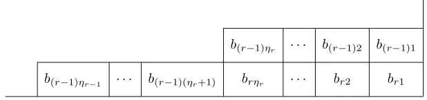
Lemma 3.2. If µ ⊂λ are partitions with λ = (ab) for some a andb then there
is a unique partition η = (η1, . . . , ηr)such that cλµη 6= 0, and for this partition we
havecλ
µη= 1. Further,(λ/µ)i=ηr−i.
Proof. Consider valid extensions ofµby anyη to formλ. Asλis a rectangle, the final row of η can only be placed as illustrated in Figure 4. Then the penultimate row of η must be placed as illustrated in Figure 4. Continuing in this way we see that the choice ofη is unique, and the number of boxes in the final row ofλ/µmust equalη1, in the penultimate row must equalη2, and so on.
b(r−1)ηr · · · b(r−1)2 b(r−1)1
[image:11.595.151.460.290.363.2]b(r−1)ηr−1 · · · b(r−1)(ηr+1) brηr · · · br2 br1
Figure 4. The final two rows ofη inλ
4. A partial block result
Doran, Wales, and Hanlon [DWH99] have given a necessary condition for the existence of a non-zero homomorphism ofBn-modules from ∆n(λ) to ∆n(µ). We
will first elevate this condition to a partial block result, and then give a stronger necessary condition that must also hold for two weights to be in the same block. In section 6 we will see that this stronger condition is also sufficient for two weights to be in the same block.
Letλ be a partition. For a box din the corresponding Young diagram [λ], we denote byc(d) thecontentofd. Recall that ifd= (x, y) is in thex-th row (counting from top to bottom) and in the y-th column (counting from left to right) of [λ], then c(d) = y−x. We denote by c(λ) the multiset {c(d) : d ∈ [λ]}. If µ is a partition with [µ]⊆[λ] we writeµ⊆λ, and denote the skew partition obtained by removingµfromλbyλ/µ. We then denote byc(λ/µ) the multisetc(λ)\c(µ).
WriteXi,jfor the Brauer diagram inBnwith edges betweentand ¯tfor allt6=i, j
and with edges betweeniandj and between ¯iand ¯j. Note thatBnis generated by
the elementsXi,jtogether with the symmetric group Σn (identified with the set of
diagrams with npropagating lines). We denote byTn the elementP1≤i<j≤nXi,j
inBn. Recall also the definition of partial one-row diagrams in the proof of Lemma
2.2.
Lemma 4.1. Let µ be a partition of m with m = n−2t. For all w ∈ Vn,t and
x∈Sµ we have that
Tn(Xw,1,id⊗x) =
t(δ−1)− X
d∈[µ]
c(d) + X
1≤i<j≤n
where (i, j) denotes the element of Σn which transposes i and j. Hence for all
y∈∆n(µ) we have
Tny=
t(δ−1)− X
d∈[µ]
c(d) + X
1≤i<j≤n
(i, j)y.
Proof. This is essentially [DWH99, Lemma 3.2], together with observations in the
proof of [DWH99, Theorem 3.3].
The next result is a slight strengthening of [DWH99, Theorem 3.3] (which in turn generalises [Naz96, formula before (2.13)], which considers the case δ ∈ N). The
original results provide a necessary condition for the existence of a homomorphism between two standard modules, but can be refined to prove
Proposition 4.2. Suppose that[∆n(µ) :Ln(λ)]6= 0. Then eitherλ=µorλ∈Λrn
andµ∈Λs
n for somer−s= 2t >0. Further, we must have
µ⊆λ and t(δ−1) + X
d∈[λ/µ]
c(d) = 0.
Proof. The first part of the proposition is clear from the quasi-hereditary structure of Bn. For the second part, note that by using the exactness of the localisation
functor we have
[∆n(µ) :Ln(λ)] = [∆r(µ) :Lr(λ)]
and hence we may assume thatλis a partition ofn. In this case,Ln(λ) = ∆n(λ) =
Sλ, the lift of the Specht module for CΣ
n to Bn(δ), and so any Brauer diagram
having fewer thannpropagating lines must act as zero onLn(λ). In particular, all
theXi,j’s act as zero and hence so does Tn.
The condition thatµ⊆λnow follows by regarding ∆n(µ) as aCΣn-module by
restriction and using (3.1) which describes the multiplicities of composition factors of such a module.
For the final condition, we know by assumption that there must exist a Bn
-submoduleM of ∆n(µ) and aBn-homomorphism
φ : Ln(λ)−→∆n(µ)/M.
LetN be the Bn-submodule of ∆n(µ) containingM such that
φ(Ln(λ)) =N/M.
As N|CΣn is semisimple, we can find a CΣn-submodule W of N such that N = W ⊕M andW ∼=Sλ. By Lemma 4.1 we have for ally∈W that
Tny=
t(δ−1)− X
d∈[µ]
c(d) + X
1≤i<j≤n
(i, j)y.
But W ∼= Sλ is a simple CΣ
n-module and P1≤i<j≤n(i, j) is in the centre of
CΣn, so it must act as a scalar onW. It is well known [Dia88, Chapter 1] that this
scalar is given byP
d∈[λ]c(d). Hence we have
Tny =
t(δ−1)− X
d∈[µ]
c(d) + X
d∈[λ]
c(d)y
= t(δ−1) + X
d∈[λ/µ]
ButTn must act as zero onN and hencet(δ−1) +Pd∈[λ/µ]c(d) = 0.
By standard quasi-heredity arguments [Don98, Appendix] we deduce
Corollary 4.3. Suppose thatλ∈Λr
n andµ∈Λsn withs < r. Ifλandµare in the
same block thens=r−2t for somet∈N and
(4.1) t(δ−1) + X
d∈[λ]
c(d)− X
d∈[µ]
c(d) = 0.
Whent= 2 [DWH99] gave a necessary and sufficient condition for the existence of a standard module homomorphism. From their results we obtain
Theorem 4.4. Suppose that µ⊂λwith|λ/µ|= 2. Then dim Hom(∆n(λ),∆n(µ))≤1
and is non-zero if and only if λ and µ satisfy (4.1) with λ/µ 6= (12). Indeed, if
λ/µ= (12)then
[∆n(µ) :Ln(λ)] = 0.
Proof. It is enough to consider the case when λ ⊢ n, as the general case follows by globalisation. Ifλandµdo not satisfy the required conditions then there is no composition factorLn(λ) in ∆n(µ) (and hence no homomorphism) by Corollary 4.3
and the remarks after [DWH99, Theorem 3.1]. In the remaining cases the existence of such a homomorphism was shown in [DWH99, Theorem 3.4]. By the remarks after [DWH99, Theorem 3.1] the multiplicity of the simple module ∆n(λ) in ∆n(µ)
is 1, and the dimension result is now immediate.
The next result is a strengthening of Proposition 4.2.
Proposition 4.5. Suppose that [∆n(µ) : Ln(λ)] 6= 0. Then there is a pairing of
the boxes in λ/µsuch that the sum of the content of the boxes in each pair is equal to1−δ.
Proof. We use induction onn; the casen= 2 is covered by Proposition 4.2. Thus we assume that the result holds forn−1 and will show that it holds forn.
If [∆n(µ) :Ln(λ)]6= 0 then by Proposition 4.2 we know thatµ⊆λand
(4.2) t(δ−1) + X
d∈[λ/µ]
c(d) = 0
where 2t = |λ| − |µ|. Now suppose, for a contradiction, that there is no pairing of the boxes of [λ/µ] satisfying the condition of the proposition. By localising we may assume thatλis a partition ofn, so that Ln(λ) = ∆n(λ). Thus ∆n(µ) has a
submoduleM such that ∆n(λ)֒→∆n(µ)/M.
The partitionλhas a removable boxǫi of contentssay and by Proposition 2.7
we have a surjection indn−1∆n−1(λ−ǫi)→∆n(λ). Hence we have
Hom(indn−1∆n−1(λ−ǫi),∆n(µ)/M)6= 0
and so by Frobenius reciprocity we have
Hom(∆n−1(λ−ǫi),resn(∆n(µ)/M))6= 0.
This implies that ∆n−1(λ−ǫi) =Ln−1(λ−ǫi) is a composition factor of resn(∆n(µ)).
Now using Proposition 2.7 we see that either
or
(ii) the weightµhas an addable boxǫjsuch that [∆n−1(µ+ǫj) :Ln−1(λ−ǫi)]6= 0.
We consider each case in turn.
In case (i), Proposition 4.2 implies that [µ−ǫj]⊆[λ−ǫi] and
t(δ−1) + X
d∈[λ/µ]
c(d)−c(ǫi) +c(ǫj) = 0.
Hence from (4.2) we must have
c(ǫj) =c(ǫi) =s
and by induction we can find a pairing of the boxes in (λ−ǫi)/(µ−ǫj) such that
the sum of the content of the boxes in each pair is equal to 1−δ. But as multisets
c((λ−ǫi)/(µ−ǫj)) =c(λ/µ)−c(ǫi) +c(ǫj) =c(λ/µ)
and hence there is such a pairing for the boxes of λ/µ. This gives the desired contradiction.
Now consider case (ii). Hereµhas an addable boxǫjsuch that [µ+ǫj]⊆[λ−ǫi]
and
(t−1)(δ−1) + X
d∈[λ/µ]
c(d)−c(ǫi)−c(ǫj) = 0.
Comparing with (4.2) we deduce that
c(ǫj) +c(ǫi) = 1−δ.
By induction there is a pairing of the boxes of (λ−ǫi)/(µ+ǫj) satisfying the
condition of the Proposition. But as multisets
c((λ−ǫi)/(µ+ǫj)) =c(λ/µ) −c(ǫi)−c(ǫj)
and as observed above thec(ǫi) andc(ǫj) can be paired in the right way. Hence the
boxes ofλ/µcan be paired appropriately, which again gives the desired
contradic-tion.
When δ is even we will need a further refinement of Proposition 4.2. Given
µ⊂λ, consider the boxes with content−δ 2 and
2−δ
2 inλ/µ. If [∆n(µ) :Ln(λ)]6= 0
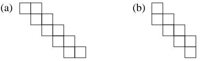
then these must be paired by Proposition 4.5, and so must be in one of the two chain configurations illustrated in Figure 5 (for some length of chain).
[image:14.595.204.411.546.609.2](a)
(b)
Figure 5. The two possible configurations of paired boxes of con-tents−δ
2 and 2−δ
2
Proposition 4.6. Suppose that [∆n(µ) :Ln(λ)]6= 0 andδ is even. If the boxes of
Proof. We will show by induction on n that in case (b) the number of columns must be even. The casen= 2 is covered by Theorem 4.4.
By repeated applications ofF we may assume thatλ⊢n. Letǫi be a removable
box ofλ. As in the proof of Proposition 4.5 we have that if [∆n(µ) :Ln(λ)]6= 0
then either
[∆n−1(µ−ǫj) :Ln−1(λ−ǫi)]6= 0
for some removable boxǫj ofµwithc(ǫi) =c(ǫj) andµ−ǫj⊂λ−ǫi, or
[∆n−1(µ+ǫj) :Ln−1(λ−ǫi)]6= 0
for some addable boxǫj ofµwithc(ǫi) +c(ǫj) = 1−δandµ+ǫj⊆λ−ǫi.
If c(ǫi) is not equal to either −δ2 or 2−δ
2 then the boxes of (λ−ǫi)/(µ−ǫj)
(respectively of (λ−ǫi)/(µ+ǫj)) of content −δ2 and 2−2δ are the same as those
boxes in λ/µ, and so the result follows by induction. Also, by our assumption on the configuration of such boxes the partition λdoes not have a removable box of content 2−2δ. Thus we may assume thatλhas only one removable boxǫiof content
−δ
2 (and hence thatλis a rectangle).
[image:15.595.222.391.348.435.2]µ
λ
Figure 6. The partitions µ ⊂ λ, with the configuration as in Figure 5(b) shaded
We have thatλandµare of the form shown in Figure 6, with [∆n(µ) :Ln(λ)]6=
0. So in particular
[resCΣn∆n(µ) :S
λ]6= 0.
By (3.1) we have
[resCΣn∆n(µ) :S
λ] = X
η even cλ
µη
and hence we must have cλ
µη 6= 0 for some even partitionη = (η1, . . . , ηr). Asλis
a rectangle Lemma 3.2 implies there is only one possibleη, and that each row of
λ/µhas lengthηi for some 1≤i≤r. Butηwas an even partition and hence these
lengths are all even, which implies that the number of columns occupied by shaded boxes in Figure 6 is also even as required. Definition 4.7. We say that λand µ are δ-balanced (or justbalanced when the context is clear) if: (i) there exists a pairing of the boxes inλ/(λ∩µ) (respectively inµ/(λ∩µ)) such that the contents of each pair sum to 1−δ, and (ii) ifδis even and the boxes with content−δ
2 and 2−δ
2 in λ/(λ∩µ) (respectively in µ/(λ∩µ))
Just as for Corollary 4.3 we can immediately deduce from Propositions 4.5 and 4.6 the following block result.
Corollary 4.8. If λandµare in the same block then they are balanced.
1 1 2 1 2 1 1 −3 −4 −2 0 4 3 2 0 −1 0 −2 −1 4 3 2 0 −1 0 1 0 −1 −2 −3 −2 −4 5
[λ] = [µ] = [τ ]=
[image:16.595.127.484.176.259.2]5
Figure 7. The diagrams [λ], [µ] and [τ] in Example 4.9(i)
Example 4.9. (i) Letλ= (6,42,2,1),µ= (5,22),τ =λ/(λ∩µ), andδ= 1. The diagrams [λ], [µ], and [τ] are illustrated (with their contents) in Figure 7. Clearly
X
d∈[λ]
c(d)− X
d∈[µ]
c(d) = 0
and hence λ and µ satisfy the conditions in Corollary 4.3. However, there is no pairing of the boxes in [τ] such that the content of each pair sums to zero, and henceλandµcannot lie in the same block.
(ii) Letα= (5,44), β = (5,14),γ =α/(α∩β), andδ= 2. The diagrams [α], [β],
and [γ] are illustrated (with their contents) in Figure 7. In this case the boxes in [γ] can be put into pairs such that each pair sums to 1−δ= −1, but the boxes with contents 0 and−1 are in configuration (b) from Figure 5, and occupy an odd number of columns. Henceαandβ cannot lie in the same block.
1 2 3 4
1
1 2 1 2
1 −2 0 0 −1 −2 4 3 2 0 −1 0 1 0 −1 −2 −3 −2 −4 0 −1 −3 −3 −4 −3 0 0 −1 −1 −2 −1 −2 −1 [β] =
[α] = [γ ]=
Figure 8. The diagrams [α], [β] and [γ] in Example 4.9(ii)
By Corollary 4.8 weights which are not balanced will lie in different blocks. Hence for aBn-moduleX we will denote by prλX the direct summand ofX with
composition factorsLn(µ) such thatµandλare balanced.
Lemma 4.10. Suppose thatλ⊢n andǫi∈rem(λ).
(i) There exists aBn-module X and a short exact sequence
0−→X −→prλindn−1∆n−1(λ−ǫi)−→∆n(λ)−→0.
Here X∼= ∆n(λ−ǫi−ǫj)if(λ−ǫi−ǫj, λ)is a balanced pair orX = 0if no such
[image:16.595.138.474.472.554.2](ii) If
Hom(prλindn−1∆n−1(λ−ǫi),∆n(µ))6= 0
then[∆n(µ) :Ln(λ)]6= 0.
Proof. (i) The existence of such a sequence, and the form ofX, follows from Propo-sition 2.7 and Corollary 4.8. To see that the sequence is non split, we proceed by induction on |λ|, the case where λ =∅ being clear. By Frobenius reciprocity we have
(4.3)
Hom(∆n−1(λ−ǫi),res ∆n(λ−ǫi−ǫj))∼= Hom(ind ∆n−1(λ−ǫi),∆n(λ−ǫi−ǫj))
By (2.2) and Lemma 2.6(ii) the left-hand side equals
Hom(∆n−1(λ−ǫi),ind ∆n−2(λ−ǫi−ǫj)).
As ∆n−1(λ−ǫi) is simple, we have by the induction hypothesis and Theorem 4.4
that this Hom-space is one dimensional. Hence the right-hand side of (4.3) is also one dimensional, which by another application of Theorem 4.4 implies that the desired sequence is non-split as required.
(ii) Note that the head ofX cannot occur in the head of prλindn−1∆n−1(λ−ǫi)
as radXcannot be extended by ∆(λ) =L(λ). Now (ii) is an immediate consequence
of (i).
5. Computing some composition multiplicities
So far we have concentrated on conditions which imply that weights lie in dif-ferent blocks of the algebra. In this section we will find certain pairs of weights which do lie in the same block, which we will demonstrate by determining cer-tain composition factors of standard modules, and homomorphisms between such modules.
We first consider the special case where the skew partitionλ/µis itself a partition. For such pairs we will be able to show precisely when Ln(λ) is a composition
factor of ∆n(µ). We first give a necessary condition, in Proposition 5.1, which is a
generalisation of [DWH99, Corollary 9.1] (the latter only considers the caseµ=∅
and homomorphisms rather than composition factors).
Proposition 5.1. Let µ⊂λbe partitions such thatν =λ/µis also a partition. If [∆n(µ) :Ln(λ)]6= 0
thenν = (ab)wherea is even andb=δ+a−1 + 2c, wherec is the content of the
top left-hand box ofν. Moreover, in this case we have [∆n(µ) :Ln(λ)] = 1.
Proof. As usual, by localisation we can assume that λ is a partition of n. First suppose that [∆n(µ) : Ln(λ)]6= 0. As Ln(λ) is simply the lift of Sλ forCΣn, we
have that
[resCΣn∆n(µ) : S
λ]6= 0.
By (3.1) we have
[resCΣn∆n(µ) :S
λ] = X
η⊢2k η even
Hence we see thatν must be an even partition, and by Lemma 3.1 that [∆n(µ) :
Ln(λ)] = 1.
On the other hand, using Proposition 4.5 we know that there is a pairing of the boxes of ν such that the sum of the content of the boxes in each pair is equal to 1−δ. Clearly we have a submoduleM of ∆n(µ) and an embedding
∆n(λ)֒→∆n(µ)/M.
Ifǫi is any removable box of λthen we have a surjective homomorphism
indn−1∆n−1(λ−ǫi)→∆n(λ).
Composing these maps we see that
Hom (indn−1∆n−1(λ−ǫi),∆n(µ)/M)6= 0
and so by Frobenius reciprocity we have
Hom (∆n−1(λ−ǫi),resn(∆n(µ)/M))6= 0.
Thus
[resn∆n(µ) :Ln−1(λ−ǫi)]6= 0
and hence eitherµmust have a removable boxǫj such that
[∆n−1(µ−ǫj) :Ln−1(λ−ǫi)]6= 0
orµmust have an addable box ǫj such that
[∆n−1(µ+ǫj) :Ln−1(λ−ǫi)]6= 0.
In the first case we haveµ−ǫj⊂λ−ǫiand hencec(ǫj) =c(ǫi). However, asλ/µ
is a partition this is impossible, as no removable box inµcan have the same content as some box in λ/µ. Hence we must be in the second case with µ+ǫj ⊂λ−ǫi,
so in factǫj must be a box in ν =λ/µ. Asν is a partition, there is only one such
addable box and its content is given byc. Thus we must have
c(ǫi) = 1−δ−c.
Now, ifν =λ/µhad another removable box then it would have to have the same content. But different removable boxes have different contents. Henceν can only have one removable box, i. e. it is a rectangleν = (ab), whereais even asν must
be an even partition. The content of the only removable box of ν inside of λ is given byc+a−1−(b−1) =c+a−band this must be equal to 1−δ−c. Hence we get
b=δ−1 +a+ 2c
as required.
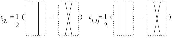
We will show that the condition in Proposition 5.1 is also sufficient. This gen-eralises [DWH99, Theorem 9.2], which again only considers homomorphisms and the caseµ=∅. Before doing this we will review some standard symmetric groups results which we will require. Details can be found in [Ful97, Chapter 7].
We will need to consider a set of idempotents{eλ : λ⊢n} in CΣn, such that
CΣneλ∼=Sλ. We will choose
(5.1) eλ= f
λ
n!
X
σ∈Cλ X
τ∈Rλ
wherefλ = dimSλ,C
λ is the column stabiliser of [λ] andRλ is the row stabiliser
[image:19.595.160.452.163.229.2]of [λ]. For example e(2) and e(1,1) (regarded as elements of B2) are illustrated in
Figure 9.
= 1
_
2
e
(2)
e
(1,1)= 1
_
2
(
(
+
)
−
)
Figure 9. The elementse(2) ande(1,1)
We will also need the fact that indCΣa+b
C(Σa×Σb)(S
µ⊗Sν)∼= M
λ⊢(n+m)
cλµνSλ.
As all these group algebras are semisimple, this implies by Frobenius reciprocity that
(5.2) resCΣn
C(Σa×Σb)S
λ∼= M
µ⊢a, ν⊢b
cλµν(Sµ⊗Sν).
Particular values ofcλ
µν which we will need are those whereν = (2), respectively
ν = (1,1). In these cases cλ
µν is at most 1, and is non-zero precisely when λ/µ
consists of two boxes in different columns, respectively different rows.
Theorem 5.2. Suppose that µ ⊂ λ and λ/µ = ν = (ab). If a is even and b =
δ−1 +a+ 2c wherec is the content of the top left box ofν then [∆n(µ) : Ln(λ)] = 1.
Moreover, if λ⊢nthen
HomBn(Ln(λ),∆n(µ))∼=C.
Proof. We can assume without loss of generality thatλ⊢n. We have seen in the proof of Proposition 5.1 that [resCΣn∆n(µ) : S
λ] = 1. LetW =e
λ∆n(µ), which
is isomorphic to Sλ as a Σ
n-module. To show this is in fact a Bn-submodule of
∆n(µ), it will be enough to show thatXi,jW = 0 for all 1≤i < j≤n. Indeed, it
is enough to show that this holds for a single choice ofiandj, as
σXi,jσ−1=Xσ(i),σ(j)
for allσ∈Σn.
So let us fixiandj with 1≤i < j ≤nand use the embedding Σn−2×Σ2⊂Σn
where Σ2 is the symmetric group on {i, j} and Σn−2 the symmetric group on
{1, . . . , n} \ {i, j}. By (5.2) and the remarks following we have resC(Σn−2×Σ2)W ∼=
M
α⊢n−2
(Sα⊗S(1,1)) M
β⊢n−2
(Sβ⊗S(2))
The mapXi,j : ∆n(µ)−→∆n(µ) is aCΣn−2×CΣ2-homomorphism. Note that
we haveXi,j(∆n(µ))⊂U whereU is the span of all elements of the formXw,1,id⊗x
wherew has an arc betweeni andj and x∈Sµ. RegardingU as aB
n−2-module
acting on the strings excluding i and j it is easy to see that U is isomorphic to ∆n−2(µ), and the restriction of this action toCΣn−2 is the same as restriction to
the action of the first component ofCΣn−2×CΣ2regarded as a subalgebra ofBn.
Also, it is clear that Xij kills the element e(1,1) in Figure 9, and hence kills the
simple moduleS(1,1). Combining these observations with (3.1) we deduce that, as
aCΣn−2×CΣ2-module,U decomposes as U =M
τ
cτ(Sτ⊗S(2))
where
cτ =
X
τ⊢n−2
ηeven
cτµη.
Consider the restriction Xi,j : W −→ U. We want to show that Xi,jW = 0.
Look at the simple summands of W. Every summand of the formSα⊗S(1,1) is
sent to zero as it does not appear inU. Moreover, ifµis not contained inβ then
Sβ⊗S(2) is sent to zero asU only contains simple modulesSη⊗S(2) withµ⊂η.
So we only need to show that
Xi,j(Sβ⊗S(2)) = 0
for any β ⊢ n−2 with µ ⊂β and β obtained from λ by removing two boxes in different columns. But there is only one suchβ, namely the partition obtained from
λby removing two boxes from the last row of ν, i.e β/µ = (ab−1, a−2), and by
Lemma 3.1 the coefficient ofSβ⊗S(2) in U equals 1.
WriteW =V ⊕Y whereV =Sβ⊗S(2). AsV is simple, eitherX
i,j embedsV
intoU orXi,jV = 0. Label the boxes of the partitionλwith the numbers 1,2, . . . , n
starting with the first row from left to right, then the second row from left to right, etc., until the last row. Say that the last box of the partitionν = (ab) inside ofλ
is labelled by l. Up until nowXi,j was arbitrary; we now fixi=l−1 and j =l
and we want to show thatXl−1,lV = 0.
Fix a partial one-row diagramw0 with t arcs defined as follows: suppose the
u-th row ofν inside ofλis labelled byxu, xu+ 1, . . . , xu+a−1 for 1≤u≤b, as
illustrated in Figure 10. Thenw0 is defined to have arcs{xu, xu+ 1},{xu+ 2, xu+
3}, . . .{xu +a−2, xu+a−1} for 1 ≤ u ≤ b. (Note that xb+a−1 = l.) We
will represent elements of Vn,t by adding bars to the Young tableau joining each
pair of nodes connected by an arc. Thus the element w0 will be represented by
the diagram in Figure 11. Usually we will only represent the boxes ofν in such a diagram.
Now consider the element of ∆n(µ) given byXw0,1,id⊗xfor somex∈S
µ. Then
eλ(Xw0,1,id⊗x)∈W, so it decomposes as
eλ(Xw0,1,id⊗x) =v+y
1
2
...
...
...
...
x
1x
1+1
x
2x
2+1
...
...
...
...
...
1
x
...
...
+a−1
−1
+a
x
2l
λ
1+1
b
x
b
x
n
...
...
...
...
...
...
...
...
...
...
...
...
...
...
...
...
...
...
...
...
...
...
[image:21.595.198.413.115.292.2]...
...
Figure 10. The labelling ofλ, withν shaded andµunshaded
.... .... .... ....
....
....
.... ....
Figure 11. A diagrammatic representation of the elementw0
ofXw0,1,id⊗xinXl−1,lv. We will show that it is a non-zero multiple of
δ−1 +a−b+ 2c.
Hence, asvis independent ofδwe see thatv6= 0, but whenδ−1 +a−b+ 2c= 0, we haveXl−1,lv = 0. ThusXl−1,l cannot embedV into U and so it must map V
to zero.
Using the labelling of the boxes of λ defined above, we will identify the row and column stabilisers Rλ and Cλ as subgroups of Σn, the symmetric group on
{1, . . . , n}. From (5.1) we have
eλ(Xw0,1,id⊗x) =
fλ
n!
X
σ∈Cλ X
τ∈Rλ
sgn(σ)στ(Xw0,1,id⊗x),
and so
Xl−1,leλ(Xw0,1,id⊗x) =
fλ
n!
X
σ∈Cλ X
τ∈Rλ
[image:21.595.215.395.332.475.2]We want to find the coefficient of Xw0,1,id⊗x in this sum. We consider several
cases.
Case 1: Suppose thatστ Xw0,vk,id has an arc{l−1, l}.
In this caseXl−1,lστ(Xw0,1,id⊗x) =δστ(Xw0,1,id⊗x). If we wantστ(Xw0,1,id⊗
x) to be in span{Xw0,1,id⊗S
µ} then we must have
τ=τ1τ2 withτ1∈Rµ⊂λ, τ2∈R0λ
σ=σ1σ2 withσ1∈Cµ⊂λ, σ2∈Cλ0
where Rµ⊂λ denotes the subgroup of Rλ (isomorphic to Rµ) which preserves the
rows ofµand fixes everything inν andR0
λ denotes the subgroup ofRλ which fixes
Xw0,1,idas a diagram (i.e. fixes all but thetnorthern arcs, which may be permuted
amongst themselves and be reversed). In a similar way we defineCµ⊂λ andCλ0.
Setr=|R0
λ|. As theacolumns ofν are paired by the bars inw0, and each pair
of such columns may be permuted freely by C0
λ we have|Cλ0|= (b!)a/2. Moreover
sgn(σ2) = 1 as σ2 is an even permutation (as it is made up of pairs of identical
permutations, corresponding to the paired ends of a bar) and so sgn(σ) = sgn(σ1).
Hence in this case we get the contribution
fλ
n!
X
σ2∈Cλ0
X
σ1∈Cµ⊂λ X
τ2∈R0λ
X
τ1∈Rµ⊂λ
sgn(σ1σ2)σ1σ2τ1τ2(Xw0,1,id⊗x)
= f
λ
n!
X
σ2∈Cλ0
X
τ2∈R0λ
σ2τ2(Xw0,1,id⊗
X
σ1∈Cµ⊂λ X
τ1∈Rµ⊂λ
sgn(σ1)σ1τ1(x))
= f
λ
n!
|µ|
fµ
X
σ2∈Cλ0
X
τ2∈R0λ
σ2τ2(Xw0,1,id⊗eµ(x))
= f
λ
n!
|µ|
fµr(b!) a/2(X
w0,1,id⊗x)
using for the second equality the isomorphismsCµ⊂λ ∼=Cµ and Rµ⊂λ ∼=Rµ, and
for the final equality the fact thateµ(x) =xfor allx∈Sµ.
Case 2: Suppose that neitherl−1 norl is part of an arc inστ Xw0,1,id.
In this caseXl−1,lστ Xw0,1,idhast+1 arcs in the top row and soXl−1,l(Xw0,1,id⊗
x) = 0.
Case 3: Suppose that inστ Xw0,vk,id there are arcs{l−1, i}and{l, j}.
In this case,Xl−1,lστ Xw0,1,id is obtained from στ Xw0,1,id by replacing the arcs
{l−1, i} and {l, j} by the arcs {i, j} and {l−1, l}. Hence if we want to have
Xl−1,lστ(Xw0,1,id⊗x) lying in span{Xw0,1,id⊗S
µ} then{i, j}must be an arc of
wandi=j±1. Here we consider two subcases.
Subcase 3(a): First assume that the pair{i, j}is not in the last double column. Then τ =τ2τ1 with τ1 ∈Rµ⊂λ and τ2 ∈τ R˜ 0λ, where ˜τ = (u−1, v) or (u, v) such
that v is a box ofν in the same column as l (possiblyl itself) anduis the box of
ν in the same row asv and in the same column as max(i, j). An example of such a situation is illustrated in Figure 12.
Thus we haveb choices for v and (a2 −1) choices for the position of{i, j} (and hence of u), and so there are 2b(a2 −1) choices for ˜τ. Hence there are 2rb(a2−1) choices for τ2. Nowσ = σ2σ1 where σ1 ∈ Cµ⊂λ, and σ2 permutes the pairs in
{i, j }
u
v
{
τ
σ
}
[image:23.595.165.444.118.215.2]l−1,l
Figure 12. An example of subcase 3(a)
double column containing{j−1, j}, it can permute the pairs in any way (as{j−1, j}
can be any pair in this double column). So we get (b!)a2−2(b−1)!b! possibilities
forσ2. Note also thatσ2 is always an even permutation and so sgn(σ) = sgn(σ1).
Thus in this subcase, we get a contribution of
fλ n! 2r b(
a
2 −1) (b!)
(a
2−2)(b−1)!b!X
w0,1,id⊗
X
σ1∈Cµ⊂λ X
τ1∈Rµ⊂λ
sgn(σ1)σ1τ1(x)
= f
λ
n!
|µ|!
fµ r(a−2) (b!)
a
2X
w0,1,id⊗x
where the equality follows as in Subcase 1.
Subcase 3(b): Next assume that the pair{i, j} is in the last column. We must haveτ =τ2τ1 whereτ1∈Rµ⊂λ andτ2∈R0λ. Alsoσ=σ2σ1whereσ1∈Cµ⊂λ and
σ2∈(j, l)Cλ0. We haveb−1 choices for j being a box ofν in the same column as
l. Note that in this case sgn(σ2) = −1 and so sgn(σ) =−sgn(σ1). Hence arguing
as in Subcases 1 and 3(a) we get a contribution of
−f
λ
n!
|µ|!
fµ r(b−1) (b!)
a
2 X
w0,1,id⊗x.
Case 4: Suppose that inστ Xw0,1,idthere is a link froml−1 toi, say, andl is not
part of an arc (or vice versa).
In this case Xl−1,lστ Xw0,1,id is obtained from στ Xw0,1,id by replacing the arc
{i, l−1}(or{i, l}) with the arc{l−1, l}andiis not part of an arc any more. So, if we want to haveXl−1,lστ Xw0,1,idin span{Xw0,1,id⊗S
µ}thenicannot be one of
the boxes ofν. There are various potential subcases that can arise. After action by an element ofRµ⊂λ the elementimay be in any box in the same row of µ. There
are three cases: (a)iis now to the left of the first column ofν; (b)iis aboveν but not abovel−1 orl; (c)iis abovel−1 orl.
Subcase 4(a): First, assume that the boxiis in a column to the left ofν inλ. In this case,τ=τ2τ1whereτ1∈Rµ⊂λ (as we have already acted by such an element
to putiin this case above) and τ2∈(v−1, u)Rλ0, orτ2∈(v, u)R0λ where v is any
box inν in the same column asl anduis the box ofµin the same row asv and in the same column asi. An example of such a situation is illustrated in Figure 13.
Let c1 be the number of columns of λto the left of ν. Then there are 2r b c1
possible choices ofτ2. Nowσ=σ2σ1whereσ1∈Cµ⊂λ(asiis an arbitrary element
in its column of µ) andσ2 permutes the pairs in each of the first (a2 −1) double
v
{l−1, l
τ
σ
i
[image:24.595.126.487.116.215.2]u
}
Figure 13. An example of subcase 4(a)
v to l and then permutes the other pairs arbitrarily. Note that sgn(σ1) = sgn(σ).
Hence (arguing as in earlier cases) we get a contribution of
fλ
n!
|µ|!
fµ 2r b c1(b!) (a
2−1)(b−1)!X
w0,1,id⊗x
=f
λ
n!
|µ|!
fµ r(b!)
a
22c
1Xw0,1,id⊗x.
Subcase 4(b): Suppose that i is a box of µ which is above some column of ν
but to the left ofl−1. Then the only way to use row and column permutations not involving Rµ⊂λ (which we have already used to position i) to connect i and
l (or l−1) is by some pairτ and σ similar to that shown in Figure 14. But (as illustrated) any such pair does not preserve the remaining edges in ν. Hence this subcase cannot arise.
{l−1, l
i
τ
σ
}
Figure 14. An example of the impossibility of subcase 4(b)
Subcase 4(c): Finally we are left with the subcase where after action byRµ⊂λ
the element i is in a box of µ which is either in the same column as l−1 or in the same column asl. In this case τ =τ2τ1 where τ1 ∈Rµ⊂λ andτ2∈Rλ0. Also,
σ= σ2σ1 where σ1 ∈Cµ⊂λ (as i is an arbitrary element in its column ofµ) and
either σ2∈(i, l)Cλ0or σ2 ∈(i, l−1)Cλ0. Ifc2 is the number of columns aboveν in
λthen there are 2c2choices for the position ofi. Note that here sgn(σ2) =−1 and
so sgn(σ) =−sgn(σ1). Hence, in this case we get a contribution of
−f
λ
n!
|µ|!
fµ r(b!)
a
22c
[image:24.595.138.475.431.545.2]Note that the final sets of permutations obtained in Subcases 4(a) and 4(c) are disjoint, so there is no double counting in these contributions. Now on adding up all contributions from Cases 1–4 we see that the coefficient ofXw0,1,id⊗xinside of
Xl−1,leλ(Xw0,1,id⊗x) is given by
fλ
n!
|µ|!
fµ r(b!)
a
2 (δ−1 +a−b+ 2(c
1−c2)).
The content of the top left box of the partitionν inside the partitionλis given byc= (c1+ 1)−(c2+ 1) =c1−c2. Thus we have proved that this coefficient is a
non-zero multiple of (δ−1) +a−b+ 2c as required.
6. The blocks of the Brauer algebra
In section 4 we saw that a necessary condition for two weightsλ and µ to be in the same block was that the pair was balanced. We will now show that this condition is also sufficient. The key idea will be to construct from any partition
λ in a balanced pair with some µ ⊂ λ a partition ν ⊂ λ and a homomorphism connecting ∆n(λ) and ∆n(ν). This will allow us to proceed by induction.
Given a partitionλwe denote by add(λ) the set ofaddableboxes ofλ(i.e. the set of boxes which may be added toλsuch that the new shape is still a partition). Similarly we denote by rem(λ) the set ofremovable boxes of λ. Ifµ⊂λthen we denote the set of boxes in rem(λ) which are also boxes ofλ/µby rem(λ/µ). Distinct boxes in add(λ) (respectively in rem(λ)) have distinct contents, and we will identify such boxes by their contents. We will order the boxes inλwith a given content by saying that boxǫissmallerthan boxǫ′ ifǫappears on an earlier row thanǫ′. Definition 6.1. Suppose thatµ⊂λis a balanced pair. For each ǫi ∈rem(λ/µ)
we wish to considerµi, thei-maximal balanced subpartition betweenµ andλ. This
is the maximal partition µi ⊂ λ such that µi does not contain ǫ
i and λ and µi
form a balanced pair. We will constructµi by recursively defining a series of skew
partitions (λ/µi)
j which will eventually equal the skew partition λ/µi. There is
by the pairing condition a maximal box (i.e. all others smaller) with contentc(ǫ′
i)
such thatc(ǫi) +c(ǫ′i) = 1−δ. Let (λ/µi)0={ǫi, ǫ′i}. Given (λ/µi)m, we set
(λ/µi)m+1= (λ/µi)m∪Am+1∪A′m+1
whereAm+1 is the set of boxesǫinλsuch thatǫis to the right of or below a box
in (λ/µi)
m, andA′m+1is the set of boxes ǫ′ in (λ/µ) such thatc(ǫ) +c(ǫ′) = 1−δ
for some ǫ∈Am+1 and ǫ′ is maximal with such content among the boxes of λ/µ
not already in (λ/µi) m.
This iterative process eventually stabilises, and we obtain (λ/µi)
t which is a
(possibly disconnected) subset of the edge ofλ/µ, having width one. (In particular it does not contain two boxes with the same content.) If δ is even and (λ/µi)
t
does not contain a vertical pair of boxes with content 2−δ
2 and −
δ
2, or δ is odd
and (λ/µi)
t does not contain a box of content 1−2δ then we set λ/µi = (λ/µi)t.
Otherwise ifδ is even we set
(6.1) (λ/µi)t+1= (λ/µi)t∪ {x, y}
wherex, y are the maximal boxes inλof content 2−2δ and −δ
2 not in (λ/µi)t, and
ifδis odd we set
where z is the maximal box in λ of content 1−2δ not in (λ/µi)
t. This new skew
partition is not necessarily stable under the addition of boxes A andA′ as above,
and we repeat that process again until the skew partition eventually stabilises at some steps. We then setλ/µi= (λ/µi)
s. Thusλ/µi is a removable subset ofλ/µ
having width at most two (so at most two boxes with any given content).
−3
−2
−1
0
1
2
3
4
0
1
2
3
−1
(a)
5
(b)
2
1
0
−2
−4
0
0
0
1
1
1
2
2
3
3
4
−1
−2
−2
−3
−3
5
−4
2
−1
4
1
0
−1
−5
6
[image:26.595.170.446.194.303.2]−4
Figure 15. Two examples of theλ/µi construction
Example 6.2. We will now consider several examples of this construction. First let λ = (6,5,5,2,1) and µ = (6,4,1); this is a balanced pair for δ = 2. If ǫi
is any of the removable boxes in Figure 15(a), then λ/µi is the shaded region shown. For an example where the resulting skew partition is connected, consider
λ= (7,6,5,5,2,2) and µ= (7,4,4,1,1). This is a balanced pair for δ= 2. If ǫi is
any of the removable boxes inλ/µthen the skew partitionλ/µiis the shaded region
shown in Figure 15(b). In this case there is a pair of boxes in the skew partition with contents 2−2δ and −δ
2 (i.e. 0 and −1), but we do not get a strip of width 2
because these boxes are not vertically aligned.
For an example of the full iterative process consider λ= (7,6,44,12) and µ=
(4,34). This is a balanced pair for δ = 2, and after the first part of the iterative
process the skew partition stabilises into the lightly shaded region shown in Figure 16(a). However, we now have a vertical pair in the skew partition with contents
2−δ
2 and −
δ
2 (i.e. 0 and −1). Thus we have to apply (6.1), and add the darkly
shaded boxes with content 0 and −1 to this skew partition. The complement of this is no longer a partition, so we remove the remaining darkly shaded region by one further application of the iterative procedure.
Definition 6.3. We now wish to define amaximal balanced subpartition between
µand λ, which we will denote byλ/µ′. Having constructed a skew partitionλ/µi
for each removable boxǫi of λ, we partially order this collection by inclusion. We
then takeλ/µ′ to be some minimal element of this set.
Example 6.4. For a non-trivial example of this choice, considerλ= (7,62,5,42,2)
and µ = (5,3,23,1). This is a balanced pair for δ = 1, but has several different
associated skew partitions. If we takeǫi to be one of the removable boxes labelled
by 6 or−5 then λ/µi equals the entire shaded region in Figure 16(b). However,
if we takeǫj to be any of the other removable boxes thenλ/µj consists of the six
darkly shaded boxes. As λ/µj ⊂ λ/µi, we take λ/µ′ to equal λ/µj in this case,
−3
−1
0
1
2
3
4
0
1
2
3
−1
−2
−5
−7
−6
−4
5
6
4
1
0
−1
−1
−2
−2
−2
−3
−3
−4
0
(a)
(b)
0
[image:27.595.134.459.95.257.2]0
0
0
1
1
1
1
2
2
2
3
3
3
4
4
5
5
6
−1
−1
−1
−1
−2
−2
−2
−2
−3
−3
−3
−4
−4
−5
−6 −5
Figure 16. More examples of theλ/µi construction
of content 0 between the two darkly shaded regions, then we would have to apply (6.2) and this box would have associated skew partition all of the darkly shaded region together with itself and the diagonally adjacent box with content 0.)
The importance of this construction is given by
Theorem 6.5. Ifµ⊂λis a balanced pair, then for any maximal balanced subpar-titionµ′ between µandλwe have
Hom(∆n(λ),∆n(µ′))6= 0.
Proof. As usual, we may assume that λ is a partition ofn. Pick ǫ ∈ rem(λ/µ′)
with |c(ǫ)−1−δ
2 | maximal. (Note that there are at most two such boxes.) Ifδ is
even andc(ǫ) = −2δ orc(ǫ) =2−2δ thenλ/µ′ is one of the two cases in Figure 17(a)
or (b), while if δis odd andc(ǫ) = 1−δ
2 thenλ/µ
′ is as in Figure 17(c). In each of
these cases there is a non-zero homomorphism from ∆n(λ) to ∆n(µ′) by Theorem
5.2 (or more directly by repeated applications of Frobenius reciprocity). Thus we henceforth assume we are not in any of these cases.
(a)
(b)
(c)
ε
ε
ε
ε
ε
ε
’
’
’
Figure 17. Some smallǫcases, with matched box denoted byǫ′
Suppose thatǫis paired with a maximalǫ′of content 1−δ−c(ǫ). We will assume
thatǫis above, or to the right of,ǫ′, and leave the (obvious) modifications required
for the other case to the reader.
We will be able to proceed by induction using the following claim.
Claim 6.6. (i) There is no box of contentc(ǫ)inrem(µ′).
(ii)There is a unique boxǫ′ of content1−δ−c(ǫ)in add(µ′).
(iii) If |λ/µ′| >2 then the pair λ−ǫ andµ′ +ǫ′ is balanced, and the associated
[image:27.595.214.402.504.562.2]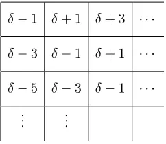


![Figure 7. The diagrams [λ], [µ] and [τ] in Example 4.9(i)](https://thumb-us.123doks.com/thumbv2/123dok_us/1618390.114884/16.595.138.474.472.554/figure-diagrams-l-u-t-example-i.webp)