Abstract: The Adomian decomposition method (ADM) proposed by George Adomian is one of the teachnique to solve linear as well as nonlinear differential equations that are encountered in the field of Physics, Biology and Engineering etc. Computation of Adomian Polynomials for each of the nonlinear terms is a vital activity when solving nonlinear problems using ADM method. In this paper the authors presents a SageMath program for computing Adomian polynomials through integer partition method for single variable case. The SageMath code developed in this paper is felt to be an efficient symbolic computation for generating Adomian polynomials. Also, SageMath package for solving nonlinear differential equations through Adomian decomposition method are presented in this paper. Examples of solving nonlinear ordinary, partial and fractional differential equations are given and the results confirm the applicability of the developed program.
Key words: Adomian decomposition method (ADM), SageMath, Nonlinear terms, Adomian Polynomials, Differential Equations.
I. INTRODUCTION
Adomian decomposition method have been used to solve nonlinear ordinary and partial differential equations and integral equations arise in Physics, Biology and various fields of Engineering [2,5]. Generation of Adomian polynomials for nonlinear term plays a vital role when solving nonlinear differential equations. George Adomian have introduced the formulae for generating Adomian polynomials for nonlinear terms [1,3,4,6]. Several authors have developed different techniques for generating Adomian polynomials and developed a package for solving nonlinear ordinary and partial differential equations through the mathematical softwares such as MATHEMATICA, MAPLE AND MATLAB[7,8,10,11,15-19]. Symbolic computation of Adomian polynomials based on Rach‟s rule through integer partition using MATLAB is developed by the authors for single variable case [24]. In this paper, the authors have developed functions in SageMath called “adomiandecomposition” for generating Adomain polynomials using decomposition of integers as the procedure presented by the authors in [24] for nonlinear terms.
Revised Manuscript Received on April 07, 2019.
M.Kaliyappan, Division of Mathematics, Vellore Institute of Technology, Chennai, India.
S.Hariharan, Department of Mathematics, Amrita Vishwa Vidyapeetham, Coimbatore, India.
In addition, the function “ adomiansol” have developed to solve nonlinear differential equations by calling the function “adomiandecomposition” to generate Adomian polynomials for nonlinear terms. This paper is organized as follows, Section 2 represents the basic procedure for generating Adomian polynomials. Decomposition of positive integers for generating Adomian polynomials was explained in detail and SageMath code for generating Adomian polynomials through symbolic computation is provided in Section 3. In Section 4, Illustrations are exhibited to solve nonlinear ordinary, partial differential and fractional differential equations symbolically using the function “adomiansol” and their results are presented .
II. ADOMIANDECOMPOSITIONMETHOD
Let us recall the basic procedure for solving differential equation using Adomian decomposition method.
Consider general form of a nonlinear ordinary differential equations
Fug(t) (1) where F is a nonlinear ordinary differential operator with linear and nonlinear terms. The equation (1) may be decomposed into the linear terms Lu+Ru and nonlinear term Nu as
g Nu Ru
Lu ,… (2) where Lu is a linear term with higher order derivative and Ru is the remainder of the linear term. Since L is a higher order derivative of the linear term, eqn (2) can be represented as
… (3)
If L is a second order linear derivative operator then (3) is equivalent to
(4)
If we assume g L t c c
u 1
2 1 0
… (5) then the solution‟ u‟ of the differential equation (1) can be
represented as a series
0
n n
u
u
(6)and the nonlinear operator Nu is decomposed as
) , ( 0 1,...,
0
n n
n u u u
A Nu
.
(7)A convenient way to generate
A
n as presented by Adomian in [2] isSolving Nonlinear Differential Equations Using
Adomian Decomposition Method Through
Sagemath
n
v
v n cvn f u A
1
0 ) ( ( ) ) ,
(
(8) Where c(v,n) are products (or sum of products) of v
components of u whose subscripts sum up to n, with the result divided by the factorial of the number of repeated subscripts. The convergence of the Adomian decomposition series and the series of the Adomian polynomials is guaranteed by Cherruault, G.Adomian and K.Abbaoui etc [9,12,13, 20-23]. The theoretical foundation of this method is discussed in detail by L.Gabet[14].
III. GENERATINGADOMIANPOLYNOMIALS
USING
DECOMPOSITION OF INTEGERS
The procedure for generating the Adomain polynomials by decomposing the positive integers is presented by the authors in [24] is given below
Step 1:
Input the positive integer n. Step 2:
Decompose n using integer partitioning Step 3:
Make the integers in the decomposed array as subscripts of u and multiply u‟s if more than one integers present (in number) in a particular sub array.
Step 4:
Count the number of repeated integers in the sub array (say k) and multiply with 1/ factorial (k) [if more than one integers are repeated in a sub array then multiply each case
separately]. Step 5:
Multiply the derivatives and then add together.
The authors developed a SageMath function for generating Adomian polynomials by applying the above procedure.
3.1 SAGEMATH PROGRAM FOR GENERATING ADOMIAN POLYNOMIALS
SageMath is a free open-source mathematical software that helps us to perform many mathematical tasks. SageMath uses Python to bind several open-source packages into one coding interface. It has been used for teaching and research in various branches of pure and applied mathematics, such as basic algebra, calculus, number theory, cryptography, numerical computation, commutative algebra, group theory, combinatory, graph theory, linear algebra etc.
Since it is an open source software program, it is one of the tool for the researchers in the under developed countries who are all working in computational techniques such as Adomian decomposition method.
The following is a SageMath program for generating Adomian polynomial
N
A .
Input: N, y2, where N is the number of Adomian polynomials
N
A
Output: Adomian Polynomial def adomiandecomposition(N,y2): x = var(“x”)
t = var(“t”) y = var(“y”) dfun = [0]*(N+1) dfun[0]=y2
for k in range(1,N+1):
dfun[k]=dfun[k-1].derivative(y1) z=decompose(N)
d1=sorted(z, key=len) l=len(d1)
Ad1=[0]*(l) Ad2=[0]*(N) Ad3=[0]*(N) l3=[0]*(l)
for k in range (0,l): l3[k]=len(d1[k]) l2=d1[0] l4=[0]*(l-1)
Ad1[0] = var(„u_%d‟%l2[0]) for k in range (1,l):
l2=d1[k] t1=len(l2) l4[k-1]=t1 t=1
for k1 in range (0,t1): t = t*var(„u_%d‟%l2[k1]) l5=sorted(l2)
count =0
while(count<t1): t2=l2.count(l5[count]) if t2>1:
count=count+t2 t=t*(1/factorial(t2)) else:
count=count+1 Ad1[k]= t.simplify_full()
l1=1
for k1 in range (2,N+1): t5=l4.count(k1) t4=0
for k2 in range (0,t5): t4=t4+Ad1[l1+k2]
l1=l1+t5 Ad2[k1-1]=t4;
Ad2[0]=Ad1[0] for k in range (0,N):
Ad3[k]=Ad2[k]*dfun[k+1] Ad3=sum(Ad3) return(Ad3)
Note: For decomposing positive integers we have called the function „decompose()‟
3.2 Python code for decomposing positive integers q = { 1: [[1]] }
def decompose(n): try:
result = [[n]]
for i in range(1, n): a = n-i
R = decompose(i) for r in R:
if r[0] <= a:
result.append([a] + r) q[n] = result
return result
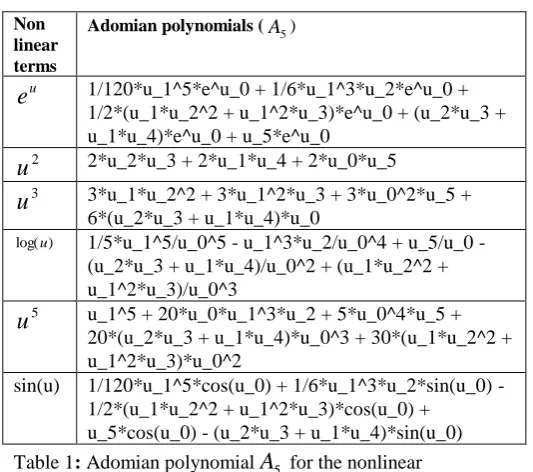
The following Table shows the calculation of Adomian polynomial
A
5 for different non-linear terms such asu
e
, 2 u ,u3 ,) log(u , 5
[image:3.595.40.307.238.474.2]u and sin(u) using the function “adomiandecomposition”
Table 1: Adomian polynomial
A
5 for the nonlinear termse
u,u
2,u
3,log(
u
)
,u
5and sin(u)IV. SOLVINGNONLINEARDIFFERENTIAL
EQUATIONS USING ADOMIANDECOMPOSITION METHOD.
Adomian polynomials which are obtained by calling the function„adomiandecomposition(N,y2)‟ to decompose the nonlinear terms are used to solve the nonlinear differential equations. We have developed a function called „adomiansol‟ to solve nonlinear differential equations.
Input:
NL= Nonlinear term LT=Linear term inic=Initial conditions nh = Non homogeneous terms
nI = Number of times of integration required( depends on the linear terms with higher order
derivatives in the given differential equations) N = Required number of terms of the series solution. Output:
Series solutions of the required nonlinear differential equations
def adomiansol(NL,LT,inic,nh,nI,N): x = var("x")
t = var("t") y = var("y") z1 = [0]*(nI) z2 = [0]*(N+1) z1=inic y=z1[nI-1] y1=nI-1
NL1=NL
for k in range (0,nI-1):
y=integrate(y,x,0,x)+z1[y1-1] y1=y1-1
for k in range(0,nI):
if(k==0):
y2=integrate(nh,x,0,x) else:
y2=integrate(y2,x,0,x)
y3=y+y2 z2[0]=y3 show(y3)
y4=NL1.substitute(u_0=z2[0]) yL=LT.substitute(u_0=z2[0])
for k1 in range (0,nI): if(k1==0):
yLL=integrate(yL,x,0,x) yNN=integrate(y4,x,0,x) else:
yLL=integrate(yLL,x,0,x) yNN=integrate(yNN,x,0,x)
z2[1]=yLL+yNN for k in range (1,N):
y5=adomiandecomposition(k,NL) t2=var('u_%d'%k)
if(yL==0): LTV=0 else: LTV=t2
for k1 in range (0,k+1): l1=k1
t1=var('u_%d'%l1)
y5=y5.substitute(t1==z2[k1])
y6=-LTV.substitute(t2==z2[k])
for k2 in range (0,nI): if(k2==0):
y8=integrate(y5,x,0,x); y7=integrate(y6,x,0,x); else:
y8=integrate(y8,x,0,x); y7=integrate(y7,x,0,x); y9=y7+y8
z2[k+1]=y9
z3=sum(z2) Non
linear terms
Adomian polynomials (A5)
u
e
1/120*u_1^5*e^u_0 + 1/6*u_1^3*u_2*e^u_0 +1/2*(u_1*u_2^2 + u_1^2*u_3)*e^u_0 + (u_2*u_3 + u_1*u_4)*e^u_0 + u_5*e^u_0
2
u
2*u_2*u_3 + 2*u_1*u_4 + 2*u_0*u_53
u
3*u_1*u_2^2 + 3*u_1^2*u_3 + 3*u_0^2*u_5 +6*(u_2*u_3 + u_1*u_4)*u_0
)
log(u 1/5*u_1^5/u_0^5 - u_1^3*u_2/u_0^4 + u_5/u_0 - (u_2*u_3 + u_1*u_4)/u_0^2 + (u_1*u_2^2 + u_1^2*u_3)/u_0^3
5
u
u_1^5 + 20*u_0*u_1^3*u_2 + 5*u_0^4*u_5 +20*(u_2*u_3 + u_1*u_4)*u_0^3 + 30*(u_1*u_2^2 + u_1^2*u_3)*u_0^2
sin(u) 1/120*u_1^5*cos(u_0) + 1/6*u_1^3*u_2*sin(u_0) - 1/2*(u_1*u_2^2 + u_1^2*u_3)*cos(u_0) +
return(z3)
The function “adomiansol” is applied to solve few nonlinear differential equations in [25] and the results are given below.
Example 1
Consider the first order nonlinear ordinary differential equation
2 ) 0 ( ,
2
y y y dx
dy
(9) The solution by ADM up to 11 terms is given by( sum of the terms , n =10)
(10) The exact solution of the given differential equation
(9) is
x
e
2
2
,
[2/2] Padé approximants of series solution (10) is [image:4.595.301.517.232.395.2](0.166667*x^2 - 1.0*x + 2.0)/(0.0833333*x^2 - 1.5*x + 1.0)
[image:4.595.49.262.349.513.2]Figure 1
Figure 1Figure 1: Comparison of the exact solution(Green), solution by ADM up to 11 terms (Blue) and (2/2) Pade approximant of ADM solution(Red dashed line) in the interval [0, 0.068]
The following procedure is used to execute the function adomiansol(NL,LT,inic,nh,nI,N) for the Example 1. y1=var(('u_0')) # Defining variable
NL=y1^2 LT=-y1 nI=1 nh=0
z = [0]*(nI) # Defining array size z[0]=2
inic=z N=10
sol=adomiansol(NL,LT,inic,nh,nI,N) print(sol)
A=plot(sol,(x,0,0.68),color="blue") es=(2/(2-exp(x)))
B=plot(es,(x,0,0.68),color="green")
ps=(0.166667*x^2 - 1.0*x + 2.0)/(0.0833333*x^2 - 1.5*x + 1.0)
C=plot(ps,(x,0,0.68),color="red", linestyle="--") D=A+B+C
show(D) Example 2
Consider the first order nonlinear ordinary differential equation
2
1, (0) 0
dy
y y
dx (11) The solution by ADM up to 6 terms is given by(sum of the
terms )
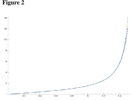
The exact solution of (11) is y = tan(x)
Figure 2
Figure 2: Comparison of the exact solution(Green dashed lines) and solution by ADM up to 20 terms (Blue) in the interval [0, 1.5]
Example 3
Consider the second order nonlinear ordinary differential equation
2
0,
(0) 1,
(0)
0
y
y
y
y
(12)The values of obtained for (12) is
The solution by ADM up to 6 terms is given by (sum of the above terms)
Example 4
Consider the second order nonlinear ordinary differential equation
3
0,
(0) 1, (0)
0
y
y
y
y
(13) Output:
The values of is obtained for (13) is
Example 5
Consider the partial differential equation
(14) The solution by ADM up to 4 terms is given by
where the operator
t L
1
One can get the above solution by doing minor modification in the “adomiansol” code.
Example 6
Consider the fractional Riccati differential equation [26, 27]
(15)
subject to the initial condition
The exact solution of (15) when α =1 is .
(16) The solution by ADM up to 3 terms is given by (sum of terms
when α =1) y = 2/15*t^5 - 1/3*t^3 + t
Figure 3
[image:5.595.46.254.102.204.2] [image:5.595.307.551.320.442.2]Figure 3: Comparison of exact solution (Green) and solution obtained using Adomian decomposition method(Red) up to 11 terms when =1.
Figure 4:
Figure 4: Plot of solutions obtained by ADM in the interval [0, 1] when α = 0.7, 0.8 and 0.9 (Red, Green and Blue)
One can get the above solution by doing minor modification in the “adomiansol” code.
V. CONCLUSION
The SageMath code presented in this paper is a simple one and also easily understandable. The main advantage of the program is its ability to generate Adomian polynomials for nonlinear terms as presented by G. Adomian. In addition to that, we have developed the function “adomiansol” to solve nonlinear ordinary differential equations using Adomian decomposition method for single linear and nonlinear terms. One can extend this concept to multivariable cases and differential equations having more nonlinear terms also. These programs will be useful for the researchers since SageMath is open source software.
APPENDIX
The syntax in SageMath used in the program is presented below:
S.No Command Name
Description
1. factorial factorial of an positive integer 2. len Length of an array
3 sorted Sorting
4 simplifyfull Simplifies the terms 5. derivative Differentiate the function 6. integrate Integrate the given function 7. count Counts the number of elements in
the array
ACKNOWLEDGMENT
We would like to thank Mr. Can Berk Güder for sharing the python code of the function decompose() in Stack Overflow.
REFERENCES
1. G. Adomian,(1992), Generalization of Adomian polynomials to functions of several variables, Computer Math.Applic., 24.(5/6) pp. 11-24
2. G. Adomian, Solving frontier problems of physics: the decomposition method, Kluwer Acad.Publ, 1994.
3. G.Adomian.(1988), A review of the decomposition method in applied mathematics, J. Math. Anal. Appl.,135, pp.501–544.
4. G.Adomian, Nonlinear stochastic operator equations, Academic Press, New York,1986.
5. G. Adomian,.(1984), A new approach to nonlinear partial differential equations, J. Math. Anal. Appl..102,420–434. 6. G. Adomian.(1997), Explicit solutions of nonlinear partial differential equations, Appl. Math Comput.88, pp.117–126. 7. R. Rach(1984), A convenient computational form for the Adomian polynomials, J. Math. Anal.Appl. 102,pp. 415–419.
[image:5.595.49.250.635.776.2]
10. S. .Guellal,. Y.Cherruault,(1994), Practical formulae for calculation of Adomians polynomials and application to the convergence of the decomposition method, Int. J. Biomed. Comput.36,pp.223–228. 11. A.M.Wazwaz (2000), A new algorithm for calculating Adomian polynomials for nonlinear operators, Appl. Math. Comput.111,pp. 53–69.
12. Y. Cherruault, G.Saccomandi,(1992), Some, New results for convergence of Adomian method applied to integral equations, Math. Comput. Modell.16(2),pp 85–93.
13. K. Abbaoui, .Y. Cherruault,.(1994), "New ideas for proving
convergence of decomposition methods", Comput. Math. Appl. 29(.7), pp.103–108.
14. L.Gabet,,(1994), The theoretical foundation of the Adomian method, Comput. Math. Appl. 27 (12), pp. 41–52.
15. Wenhai Chen, Zhengyi Lu (2004), Symbolic implementation of the algorithm for calculating Adomian polynomials, Applied Mathematics and Computation,159,pp.221–235
16. Hooman Fatootehchi, Hossein Abolghasemi(2011), On Calculation of Adomian Polynomials by MATLAB, Journal of Applied Computer Science & Mathematics, 11(5), ,pp.85-88,
17. J.S. Duan,.(2010a), An efficient algorithm for the multivariable Adomian polynomials, Applied Mathematics and Computation, 217(6), ,pp. 2456-67.
18. J.S.Duan, J.S.(2010b), Recurrence triangle for Adomian polynomials, Applied Mathematics and Computation, 216(4), 19. pp.1235-41. Duan, J.S.(2011), Convenient analytic recurrence
algorithms for the Adomian polynomials, Applied Mathematics and Computation, 217(13), pp. 6337-48
20. Y.Cherruault, (1989), Convergence of Adomian‟s method, Kybernetes,.18, pp.31–38.
21. Y. Cherruault., G.Adomian,G.(1993), Decomposition methods: a new proof of convergence, Math. Comput. Model.
Vol.18,pp.103–106. 22. K.Abbaoui,., Y. Cherruault,(1994). Convergence of Adomian‟s
method applied to nonlinear equations, Math. Comput. Model. .
20(9),, pp. 60–73. 23. K. Abbaoui,.,Y. Cherruault,.(1994),. Convergence of Adomian‟s
Method Applied to Differential Equations, Computers Math.
Application. Vol.28, No.5, pp.103-109 24. M. Kaliyappan,M,, S.Hariharan,.(2015), Symbolic Computation of
Adomian Polynomials Based on Rach‟s Rule, British Journal of Mathematics & Computer Science,5(5),pp .562-570.
25. A.M.Wazwaz, Partial differential equations and solitary waves theory, Springer, 2009.
26. Shaher Momani, Nabil Shawagfeh(2006), Decomposition method for solving fractional Riccati differential equations, Applied
Mathematics and Computation 182, pp 1083–1092.
27. Mehmet Merdan(2012), On the Solutions Fractional Riccati Differential Equation with Modified Riemann-Liouville Derivative, International Journal of Differential Equations, doi:10.1155/2012/346089
AUTHORSPROFILE
M. Kaliyappan is an Associate Professor of Mathematics in the School of Advanced Sciences at VIT Chennai, India. He has over 21 years of experience in teaching and research. His research interest includes Approximation theory, Numerical computing and Differential equations. He is currently guiding 3 Ph.D. students. He has 11 publications in International Journals.
S. Hariharan working as an Associate Professor, Department of Mathematics, Amirta School of Engineering – Coimbatore, INDIA. He completed his Doctorate degree in the field of application of wavelets in diffusion equations from Florida Institute of Technology, Melbourne, Florida. He has more than 10 years of research and teaching
![Figure 4: Plot of solutions obtained by ADM in the interval [0, 1] when α = 0.7, 0.8 and 0.9 (Red, Green and Blue)](https://thumb-us.123doks.com/thumbv2/123dok_us/8213268.263688/5.595.307.551.320.442/figure-plot-solutions-obtained-adm-interval-green-blue.webp)
