International Journal of Innovative Technology and Exploring Engineering (IJITEE) ISSN: 2278-3075, Volume-9 Issue-2, December 2019
Abstract: Inventory problem are generally classified under decision making problem where lead time plays an important role in performance and services to customers during supply and placement of order of an item orders can be placed in shorter lead time with higher price or in longer lead time with lower cost. In this paper we have formulated multi-objective inventory model with one objective of minimizing the total inventory cost and other objective of maintaining the quality of the product by discarding the defective items. The model involved the deterministic demand, lead time dependent lead time cost, holding cost, ordering cost and inspection cost for inspecting defective items. The techniques of priority goal programming and genetic algorithm are applied and the results are compared. The sensitivity analysis is explained due to restriction in cost parameter. The model is finally illustrated with a numerical example.
Keywords: Lead time, Customer service level, Goal programming, Priority goal programming.
I. INTRODUCTION
A
supply chain is a chain between all parties where its target to fulfill their customer request either directly or indirectly. The chain is not only limited to seller or buyer but it may be extended to the warehouses, retailers or even customers themselves. In an organization it includes all the functions not only limited to receiving and satisfying the customer request but also the different activities, manpower, resources, entities, etc. are included in it. It represents the sequence of delivery of the product from the source to the destination that is the customer. This sequence involves the movement of the raw material into the finished product, its transportation, and distribution to the end-user. The entities are the manufacturers, sellers, buyers, retailers, distribution centers, etc. The element of the supply chain is the function of receiving an order to meet the customer's request. Supply chain management is an essential process for every supply chain model.In recent years a seller-buyer integrated inventory problem makes a lot of focus in supply chain management. Supply chain management helps in the smooth running of goods and services in the entire chain. It consists of the movement and storage of raw materials, works in process inventory and finished goods from the source to the destination. Supply chain management maintains the relationship between the inter-organization as well as the intra-organization through
Revised Manuscript Received on December 05, 2019.
* Correspondence Author
Sandipa Bhattacharya*, Department of Mathematics, National Institute of Technology, Durgapur, West Bengal-713209, India.
Email: [email protected], [email protected]
Seema Sarkar (Mondal), Department of Mathematics, National Institute of Technology, Durgapur, West Bengal-713209, India.
Email: [email protected]
the various types of flow of product in anentire supplychain structure. It helps in collaborating with other industries in the whole world to meet their demand. Firms are realizing that the management of inventories must be efficient through the entire supply chain.
In the past, economic order quantity and economic production quantity models are independently developed from the buyers' point of view. But in the current scenario, the supply chain model is developed co-operatively in increasing productivity and preserving benefits. In this environment, the ultimate goal is to achieve global optimality. In a competitive environment, researchers make attention to improving the quality of the product and decreasing the total inventory cost.
In the present competitive market, the selling price of a product is one of the decisive factors in selecting an item. In practice, a reasonable selling price of the product has a good impact on the market whereas the higher and lower selling price refuses the demand. But rejecting demand is more appropriate for defective items.
Sometimes we overlooked the situation for advanced payment at the time of ordering of an item. It is generally seen that when a retailer places an order to the wholesaler at that moment he/she makes the demand for an advance payment. Also, it is noticed that when extra advance payment is received from a retailer then he/she gets some discount in price at the time of final payment against extra advance payment. Advance payment is a real-life situation, but in our present paper, we are not considering it. Here an attempt has been made to incorporate the lead time for delivery of an item.
For the development of our proposed model, different literatures have been studied some of which are discussed in the following section.
II. LITERATUREREVIEW
During production defective items are often produced due to malfunctioning of the machine, engaging unskilled labor, etc. In real-world, it is often observed that there may be defective items produced during production time. These defective items may be reprocessed in the manufacturing house or rejected by the customer. In all such cases, the reproduction costs are included. Therefore, it is more appropriate to include the quality-related cost in the main objective function.
The relationship between quality imperfection and lot size is approached elaborately first in the Porteus [2] and Rosenblatt and lee [14].
Porteus [2] described that in each production the system runs in control but sometimes it may go out of control, at that moment the entire produced
items may become defective.
Multi-Objective Inventory Model with
Lead-Time and Defective Items
There is a chance of probability that the unit of an item is defective. His work is the inspiration of many researchers for developing a model of quality improvement in an inventory management problem.
Rosenblatt and lee [14] discussed the time between the period of the smooth production run and the production process which goes out of control. In this paper, the authors take exponential time and identified the defective items. These imperfect products can be reworked instantaneously. This paper concluded that the presence of defective items in a lot of size inventory became smaller in size.
In another paper of Lee and Rosenblatt [4], a joint lot-sizing under the economic order quantity model was considered where they included the inspection policy under it.
Salameh and Jaber [15] analyzed an inventory situation where the quality of items is not perfect. Imperfect items are not necessarily defective; they can be used in another inventory situation. They extended their idea in economic production quantity (EPQ) model.
Chen et al. [5] developed a framework where a single EPQ model is integrated with reprocessing and rejection situation. The inspection process is performed to identify the defective and non-defective as well as the rejected items in each lot.
Hayek and Salameh [17] presented an inventory model of shortages that consider the remanufactures of defective items.
Ouyang [11] investigated the lot size, reorder point inventory model with variable lead time with partial backorders where the process of production is not perfect.
Francis Leung [8] developed economic production quantity (EPQ) model problem where the production process is imperfect. They solved their model by using geometric programming.
Freimer et al. [13] analyzed the effect of the bad quality model in an economic production environment.
Chiu [19] considered the effects of remanufacturing of defective items on the EPQ model by allowing shortages.
Urban [18] proposed a final replenishment inventory model in which demand is taken as a deterministic function of price. He extended the model with the possibility of defective items in the production process.
Ben-Daya [12] developed multi-stage lot sizing models. Lee [3] introduced an inventory cost model using investment strategies in inventory and providing maintenance in an inventory system for not producing imperfect quality products. Here, they expressed investment strategies as a function of measurable variables. This model helped the decision-makers for making decisions that how much amount would be invested in inventory and whether the investment and maintenance are necessary or not.
Ouyang et al. [10] derived an integrated seller-buyer inventory model. They considered two issues in it–trade credit and quality improvement. In this paper, the authors assumed that the seller offers trade credit to the buyer when the production process is imperfect and the rate of the defective items can be reduced by inventory investment.
Rezaei et al. [6] developed a multi-product multi-supplier supply chain model where they assumed that the received items from suppliers are not good quality. They also conclude that imperfect items are sold at a discounted price before the next shipment. They extended their model in a supplier selection problem. Hence, their formulated model is solved by using a genetic algorithm (GA).
Chen et al. [9] developed an additive model to maximize the sum of achievement degrees of all fuzzy goals. In this paper, the authors made the importance and preemptive priority of the relevant goals.
Qin [20] derived an uncertain random model on a multi-objective optimization problem involving random variables with uncertainty.
A multi-objective optimization problem is developed in Jadidi et al. [16] with three objectives: price, rejects and leads time. The problem should minimize the total objectives. In this paper, the decision-makers determine the aspiration level or an interval goal for every objective. They derived their idea for developing a new multi-choice goal programming problem where the decision-makers have the advantages for controlling their preferences.
GA is the process of evolution by implementing the strategy of survival of the fittest one. A more complicated discussion is discussed in the book of Goldberg [1]. Here in each stage a new population is created from the preceding one using the genetic algorithm operators.
Multi-objective optimization problem involves optimizing multiple objectives simultaneously. When the objectives became conflict to each other the optimal solution of the objective function are different to each other then the problem arises. In this situation the problem may solve by a set of trade-off all the optimal solutions. Deb [7] introduced pareto-optimal solution to optimize solutions of the multiple objectives concurrently. Due to multiplicity in solutions he developed an approach of population search procedure in a single or multiple objective functions which is known as evolutionary algorithm. One of the advantages is that it not only used in single or multiple objective functions but also to solve other kinds of optimization problems in a better manner than a traditional approach.
After the study of literature, we introduce an inventory model where our objective is to minimize the total costs in inventory and we extend our model by considering two goals: to reduce the total inventory cost and to improve the quality of the items by reducing the defective ones in each lot through a proper inspection process. Finally, we make a sensitivity analysis through which we obtain the sensitive changes of a particular decision variable by small changes in the parameters. The model also has been verified numerically.
III. MODELDESCRIPTION
To develop an inventory model we have taken a constrained mathematical expression which consists of various costs and our objective is to minimize the total inventory cost. Also, the model will increase the perfect quality of the items by reducing the imperfect ones, for which we have taken some certain percentage of the non-defective items where the level of percentage will be accepted below or equal to the percentage level otherwise, it will not be accepted. According to this, we have considered two goals: first, to minimize the total inventory cost and the second, to improve the quality of the products, after that we set the priority of our proposed goals using some advanced optimization techniques, where we compare our results. Finally, sensitivity analysis is applied to analyze how the different values of a set of
International Journal of Innovative Technology and Exploring Engineering (IJITEE) ISSN: 2278-3075, Volume-9 Issue-2, December 2019
specific conditions. The following assumptions are considered for the overall scenario:
Assumptions:
(i) Holding cost of the product per unit item per unit time is fixed.
(ii) Demand is a decision variable over a planning horizon. (iii) Lead time is non-zero.
(iv) Each lot of the product contains a certain percentage of defective items and defective items are rejected.
(v) The screening procedure is conducted to identify the defective and non-defective items with a unit screening cost. (vi) Available product storage space is limited.
(vii) Shortages are not allowed. Notations:
O= Ordering cost per order
H=Holding cost per unit time per unit item W=Maximum storage space available for products
𝜃1= Defective item in each lot S=Inspection cost per item
𝑅 𝐿 =Lead time crashing cost
σ=Standard deviation of the lead time demand k=Safety factor of the lead time demand v=Volume per unit of item
TC=Total inventory cost Decision variables: D=Annual demand per year L=Lead time in weeks
θ= Non-defective item in each lot Q=Lot size or Order quantity per order
IV. MODELFORMULATION
We want to minimize the objective function of the total inventory cost which is the sum of ordering cost, holding cost, lead time crashing cost, inspection cost. We represented the lead time crashing cost R(L) as a function of lead time (L), where 𝑅 𝐿 = 𝑎 ∗ 𝐿−𝑏, where a and b are the two real constants and 𝑎 > 0; 0 < 𝑏 ≤ 0.5. Under this we have taken three constraints: (i) the order quantity per order or the lot size will be the summation of defective and non-defective items, (ii) the acceptable lot can have at most defective items 4% of the lot size and (iii) the storage space is limited where the lot will be kept. Therefore, we will solve with the help of a numerical example for the above minimization problem under the three constraints using different techniques. Objective function:
Minimize
2
D Q D
TC O H k L R L S Q
Q Q
Constraints:
(i) Sum of non-defective and defective items is equal to the order quantity per order:
1
Q
(ii) Defective item should be within a certain percentage of a lot size for which lot is acceptable:
1 0.04 Q
(iii) Capacity constraint:
v Q W Numerical Examples:
The model is verified with numerical example using different techniques. For numerical computation, following parametric values are used:
O=Rs.700 per order; S=Rs. 250 per item; H=Rs. 300 per unit item per unit time; W= 600 𝑚3; v=9 𝑚3 per unit; k=3; σ=1.04; a=2; b=0.2.
Using Lingo the following values of the decision variable and the optimum cost are obtained.
Table-1: Values of the decision variable and the optimum cost:
D (units/year)
L (weeks)
θ (units)
𝜽𝟏
(units) Q (units)
TC (Rs.)
800 10 36.95 0.50 37.45 32920.12
These values indicate that supplier can order the item of 800 units and adopt a lead time of 10 weeks with a total inventory cost of Rs. 32920.12.
A. GOAL PROGRAMMING
Our inventory model is considered to be of optimization type involving two goals –
First goal: to minimize the total inventory cost and Second Goal: to improve the quality of the product
To achieve these two goals we introduce an optimization technique known as the goal programming method.
Goal Programming Formulation:
Here a non-linear goal programming model has been developed in the presence of two goals.
To reach the first goal of not exceeding the total inventory cost of Rs. 30000, the goal constraint is described as follows:
1 12 30000
D Q D
O H k L R L S Q O
Q Q U
Where O1 and U1 are respectively overachievement and underachievement of the targeted goal of Rs. 30000.
The second goal constraint of reducing the defective items less than 0.32 is presented as:
1 O2 U2 0.32
Where O2 and U2 are respectively overachievement and underachievement of the targeted goal of 0.32.
Since our objectives are to minimize total cost of inventory and the number of defective items, hence minimizing overachievements O1and O2will lead towards achievement. Therefore, present objective function is to
Minimize Z O1O2 Subject to the constraint Goal 1:
1 12 30000
D Q D
TC O H k L R L S Q O
Q Q U
Goal 2:
1 O2 U2 0.32
1
1 0.04
Q
Q
v Q W
Table-2: Values of decision variables in goal programming method:
D L θ 𝜽𝟏 Q 𝐎𝟏 𝐔𝟏 𝐎𝟐 𝐔𝟐
815 7 37.58 0.22 37.80 2718.24 0 0 0.098
It is observed that from Table-2 that the total inventory cost is overachieved by an amount of Rs. 2718.24 which shows the total cost in inventory is Rs. 2718.24 more than the targeted cost of Rs. 30000. Thus in this case total inventory cost = Rs. (30000 + 2718.24) = Rs. 32718.24.
It is observed that from Table-2 that the defective items are underachieved by an amount of 0.098 which shows the defective items is 0.098 less than the targeted goal of 0.32. Thus in this case defective items = (0.32-0.098) = 0.222.
Next, we attempt the priority goal programming method as another advanced optimization technique where we set the priority of the two goals. Our first priority is to minimize the total cost of inventory and the second is to reduce the defective items in lot size. In this case two priorities P1 andP2
are assigned to the first and second goal respectively. This indicates that P1 goal is more important than P2 goal will not
be achieved until P1 goal has been achieved.
B. PRIORITY GOAL PROGRAMMING
The formulation of Priority Goal Programming Problem is as below:
Minimize Z P1 O1P2O2
Subject to the constraint
1 12 30000
D Q D
O H k L R L S Q O
Q Q U
1 O2 U2 0.32
1
1 0.04
Q
Q
v Q W
It is noticed that the goals have been met to different extents. The result of priority goal is shown in Table-3.1 and Table-3.2 will show the results for the next goal.
Table-3.1: Values of decision variables in a first priority goal method:
D L θ 𝜽𝟏 Q 𝐎𝟏 𝐔𝟏 𝐎𝟐 𝐔𝟐
500 2 15.18 0.47 15.65 0 1.23 0.15 0
Table-3.2: Values of decision variables in a second priority goal method:
D L θ 𝜽𝟏 Q 𝐎𝟏 𝐔𝟏 𝐎𝟐 𝐔𝟐
640 3.5 23.84 0.32 24.16 0 1.25 0.48 0
It is observed that the two tables represent the data of the number of defective items, number of non-defective items, value of the underachievement and overachievement variables of the total inventory cost and number of defective items of the lot size, number of shipment, lead time, and annual demand per year. In the first table we have taken P1 as
a pre-emptive priority factor of the overachievement of the total inventory cost. We obtained the value of the underachievement variable of total inventory cost Rs. 1.23 where the value of the overachievement variable of the
number of defective items is 0.15. Consequently, in the second table we have taken P2 as a pre-emptive priority factor
of the overachievement of the number of defective items. We obtained the value of the overachievement variable of the number of defective items 0.48 and the value of the underachievement variable of total inventory cost Rs. 1.25. After observation it can say that we achieved our targeted goal by reducing the total inventory cost as well as improve the quality of the products by reducing the number of defective items in a satisfactory level.
C. NON-LINEAR OPTIMIZATION TECHNIQUE
We can solve our non-linear programming model using a very popular non-linear optimization technique known as the Genetic Algorithm (GA). The genetic algorithm is a method for solving both constrained and unconstrained optimization problems. The method repeatedly modifies a population of individual solutions. At each step, the genetic algorithm selects individuals at random from the current population which is the parents and uses them to produce the children for the next generation. The application of the geneti
c
algorithm is to solve a variety of optimization problems in which the objective function is discontinuous, non-differentiable, stochastic, or highly nonlinear. We apply this technique in our proposed inventory model for obtaining the better result than the previous technique and the results are shown in the following table (Table-4):Table-4: Values of decision variables and optimal cost using genetic algorithm technique:
D (units/year)
L (weeks)
θ (units)
𝜽𝟏
(units) Q (units)
TC (Rs.)
430 2 27.12 0.345 27.46 24925.05
We have obtained (in Table-1) the value of number of non-defective items as 36.95 units, the number of defective items is 0.50 units and the total inventory cost is Rs. 32920.12 whereas the corresponding values respectively 27.12, 0.345 and Rs. 24925.05 as obtained by using non-linear optimization technique. After a fair observation, we can compare our crisp result with the result by using the genetic algorithm where the total inventory cost will reduce from Rs. 32920.12 to Rs. 24925.05 and it will save up to Rs. 7995.07, simultaneously, it will improve the perfect quality of the product by reducing the number of defective items from 0.50 to 0.345. So we should opt for the technique of Genetic Algorithm because we can get a better result in a non-linear optimization technique than the simple linear optimization technique.
D. SENSITIVITY ANALYSIS
Sensitivity analysis is used in the business world and in the field of economics. It determines how different values of an independent variable affect a particular dependent variable under a given set of assumptions. This technique is used within specific boundaries that depend on one or more input variables. It is a way to predict the outcome of a decision
given a certain range of variables. The person doing the
International Journal of Innovative Technology and Exploring Engineering (IJITEE) ISSN: 2278-3075, Volume-9 Issue-2, December 2019
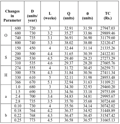
Table-5: Values of decision variables and optimal cost by changing the parameters in sensitivity analysis:
Changes in Parameter
D (units/
year) L (weeks)
Q (units)
𝛉
(units)
TC (Rs.)
O
600 720 3 32.91 31.59 27947.03 680 730 3.2 35.27 33.86 29889.46 740 735 3.1 36.91 36.90 31179.60 800 740 3.3 38.02 38.00 32120.47
S
150 450 4 32.44 31.14 21335.26 200 500 4.4 31.65 30.39 24122.81 280 530 4.5 29.40 28.23 27273.29 310 535 4.6 29.37 28.20 27605.76
H
274 555 4 31.72 30.45 26259.71 300 578 4.3 31.84 30.56 27411.34 330 610 5 32.11 31.98 28953.48 366 670 5.1 32.94 31.63 31109.21
a
1.0 680 3 34.30 32.93 29460.20 1.5 690 3.3 34.56 33.18 29753.09 2.4 700 3.4 34.83 34.81 29995.67 2.8 735 3.5 35.70 35.68 30724.60
b
0.10 730 4 35.56 34.14 30742.02 0.18 764 4.2 36.37 34.92 31448.89 0.22 768 4.3 36.47 36.45 31547.42 0.25 773 4.5 36.58 36.57 31665.13
When the annual demand is gradually increasing the total inventory cost is in increasing in nature but it will decrease the number of defective items. Similarly when we increase the lead time the number of defective items will decrease simultaneously the total inventory cost increases. Again, when we improve the number of non-defective items of the lot size it increases the total inventory cost whereas the number of defective items will reduce. As a whole, we say that we can improve the quality of the non-defective items by reducing the defective ones after the proper inspection procedure and the increasing demand will increase the total inventory cost for the entire supply chain model. The above table shows the small changes of a particular variable will change the values of the other variable at the same time by keeping the values of the remaining variable unchanged. This will give the sensitive results after the sensitive changes of the dependent variables using sensitivity analysis.
V. CONCLUSIONANDFUTURESCOPE
We have considered the problem of the supply chain model. Here, we assumed that the supplier has limited storage capacity and the received items from the supplier are not all perfect quality which does not mean that they are defective items. Simple goal programming and priority goal programming approaches are proposed here. We verify our proposed model numerically using two techniques. After comparatively study we obtain a much better result in non-linear optimization techniques than traditional optimization techniques. The model has performed the sensitivity analysis where it is observed that the effects of changes in values of an optimal solution by changing in values of one parameter or one decision variable at a time while keeping all other parameters at their original levels. In this paper, shortages are not considered but in future shortages or backlogged situations can be considered. It is the one way of approach to improve the quality of the product by minimizing the total cost but there is some other approach to improve the product quality. We have considered here only the deterministic lead time but the lead time can be taken in a
stochastic or probabilistic nature. In this paper, we consider only the demand in deterministic nature but in the real world, it is not possible. One should extend the model by considering the demand with a risk of uncertainty. We have fully rejected the defective item after the inspection process before transportation and we are not thinking about that item. But in the future research work, the rejected item might be sale in discount rates at one lot or it might be reprocessed for further use.
REFERENCES
1. . D.E. Goldberg, "Genetic Algorithms in Search, Optimization and Machine Learning", Addition-Wesley, Reading, MA, 1989. 2. E.L. Porteus, "Optimal Lot-sizing, Process Quality Improvement, and
Set-up Cost Reduction", Operational Research 34 (1986), pp. 137-144. 3. H.H. Lee, "A Cost/ Benefit Model for Investment in Inventory and Preventive Maintenance in an Imperfect Production System", Computational and Industrial Engineering 48 (2005), pp. 55-68. 4. H.L. Lee and M.J. Rosenblatt, "Simultaneous Determination of
Production Cycles and Inspection Schedules in a Production System",Management Science 33 (1987), pp. 1125-1137.
5. H.M. Wee, J. Yu, and M.C. Chen, "Optimal Inventory Model for Items with Imperfect Quality and Shortage Backordering", Omega 35(1)(2007), pp. 7-11.
6. J. Rezaei and M. Davoodi, "A Deterministic, Multi-Item Inventory Model with Supplier Selection and Imperfect Quality", Applied Mathematical Modelling 32 (2008), pp. 2106-2116.
7. K. Deb, "Multi-objective Optimization using Evolutionary Algorithms", Wiley, New York, 2001
8. K.N. Francis Leung, "A Generalized Geometric-Programming Solution to an Economic Production Quantity Model with Flexibility and Reliability Considerations", European Journal of Operational Research 176 (21) (2007), pp. 240-251.
9. Liang-Hsuan Chen and Feng-Chou Tsai, "Fuzzy Goal Programming with Different Importance and Priorities", European Journal of Operational Research 133 (2001), pp. 548-556.
10. Liang-Yuh Ouyang, Kun-Shan Wu and Chia-Huei Ho, "An Integrated Vendor-Buyer Inventory Model with Quality Improvement and Lead Time Reduction", International Journal of Production Economics 108 (2007), pp. 349-358.
11. L.Y. Ouyang, C.K. Chen and H.C. Chang, "Quality Improvement, Set-up Cost and Lead-time Reductions in Lot-size Reorder Points Models with an Imperfect Production Process", Computational Operational Research 29 (2002), pp. 1701-1717.
12. M. Ben Daya, "Multi-stage Lot-sizing Models with Imperfect Processes and Inspection Errors", Production Planning Control 10(2) (1989), pp. 118-126.
13. M. Freimer, D. Thomas and J. Tyworth, "The Value of Set-up Reduction and Process Improvement for the Economic Production Quantity Model with Defects", European Journal of OperationalResearch 173 (1) (2006), pp. 241-251.
14. M.J. Rosenblatt, H.L. Lee, "Economics Production Cycles with Imperfect Production Processes", IIE Transaction 18 (1986), pp. 48-55. 15. M.K. Salameh and M.Y. Jaber, "Economic Production Quantity Model for Items with Imperfect Quality", International Journal of Production Economics 64 (2000), pp. 59-64.
16. O. Jadidi, S. Cavalieri and S. Zolfaghari, "An Improved Multi-Choice Goal Programming Approach for Supplier Selection Problems", Applied Mathematical Modelling, Vol. 39, Issue 14 (2015), pp. 4213-4222.
17. P.A. Hayek and M.K. Salameh, "Production Lot-sizing with the Reworking of Imperfect Quality Items Produced", Production Planning Control 12(6) (2001), pp. 584-590.
18. T.L. Urban, "Deterministic Inventory Models Incorporating Marketing Decisions", Computational and Industrial Engineering 22(1) (1982), pp.85-93.
19. Y.P. Chiu, "Determining the Optimal Lot-size for the Finite Production Model with Random Defective Rate, the Rework Process and Backlogging", Engineering Optimization 35(4) (2003), pp. 427-437. 20. Zhongfeng Qin, "Uncertain random Goal Programming, Fuzzy
AUTHORSPROFILE
Sandipa Bhattacharya is PhD research scholar from Department of Mathematics of National Institute of Technology Durgapur, West Bengal, India. She received her B.Sc. degree in Mathematics from Burdwan University, West Bengal, India and Masters in Computer Applications from West Bengal University of Technology, (Presently MAKAUT) West Bengal, India. She obtained her M.Tech degree in Operations Research from Department of Mathematics of National Institute of Technology Durgapur, West Bengal, India. She has participated in many National and International Workshops and Conferences in India. Her research interests include in Operations Research, Supply Chain Management, Soft Computing and some other related fields in Applied Mathematics.
Dr. Seema Sarkar (Mondal) is Professor of Department of Mathematics, National Institute of Technology Durgapur, India. She received her B.Sc. degree in Mathematics from Presidency College (Presently Presidency University) Kolkata and M.Sc , M.Phil & PhD degree in Applied Mathematics from University of Calcutta, Kolkata. Her research interests include Geophysics, Operations Research and some other related fields. She has authored/coauthored more than 25 publications and received 'Best Paper Award' in International Conference on 'Information and Management Science' in China during August, 2010. She had also received “National Scholarship” during Secondary Examination.
Five students have completed their PhD and awarded doctorate degree under her supervision and 8 more are pursuing their doctoral study.