A Floating Probe Force Microscope With Sub-Femtonewton Resolution

(1)

A Floating Probe Force Microscope

With Sub-Femtonewton Resolution

The Harvard community has made this

article openly available.

Please share

how

this access benefits you. Your story matters

Citable link http://nrs.harvard.edu/urn-3:HUL.InstRepos:37944968

Terms of Use This article was downloaded from Harvard University’s DASH repository, and is made available under the terms and conditions applicable to Other Posted Material, as set forth at http://

(2)

©2016 - Lulu Liu

(3)

Thesis advisor: Federico Capasso Lulu Liu

A Floating Probe Force Microscope with Sub-Femtonewton

Resolution

Abstract

Forces at the femtonewton level and below are poised to be highly relevant in a

number of scientific disciplines– including studies in optics and photonics,

molecular biology, and even microfluidics. It is highly practical, if not necessary,

to perform these force measurements in liquid. But due largely to increased

thermal noise, conventional force spectroscopy methods, such as atomic force

microscopes (AFM’s), underperform in a liquid environment. The most

advanced AFM’s, for instance, are limited to a resolution of around a piconewton.

On the other hand, a new class of force microscopes utilizing a floating,

optically trapped probe, have been proposed. These instruments, including the

photonic force microscope (PFM), promise lower thermal noise thresholds, due

to a smaller profile probe. But thusfar, due to fundamental flaws in design and

methodology, they have been unable to produce thermally limited

measurements.

This document summarizes the design and development of a highly sensitive

force microscope, based on such a floating probe, which is able to measure at the

thermal limit. Thus, our force microscope’s sensitivity exceeds that of the best

current techniques in fluid by two orders of magnitude, enabling resolution of

forces below one femtonewton (f N) in 100 seconds of measurement.

(4)

Thesis advisor: Federico Capasso Lulu Liu

physical phenomena which form the basis of our work. Next, some formalism is

introduced and a background is given on force microscopy and existing

techniques. The contents of three published papers populate Chapters 5-7, and

finally, an operation manual for the instrument in its current form is provided in

(5)

Listing of figures

1.2.1 Simple dipole drawing . . . 4

1.3.1 Ashkin’s 1986 image of an optically trapped microparticle . . . . 6

1.4.1 Mie scattering geometry . . . 7

2.1.1 Sketch from Perrin’s 1909 paper . . . 16

2.3.1 Sketch of brownian motion at a molecular level . . . 18

2.4.1 Power spectral density of a free Brownian particle . . . 21

2.4.2 Schematic of an optically trapped microsphere . . . 22

2.4.3 Power spectral density of an optically trapped Brownian particle 23 2.4.4 Dynamic regimes of an optically trapped Brownian particle . . . 24

2.4.5 Low-mass approximation for power spectral density . . . 25

2.6.1 Low Reynold’s number swimmer . . . 27

3.1.1 Gaussian distribution . . . 31

3.3.1 Power spectrum and RMS noise . . . 34

4.1.1 Formation of DNA loops regulated by f N forces . . . 38

4.2.1 SEM image of an AFM cantilever . . . 40

4.2.2 Cantilever of an atomic force microscope . . . 41

4.3.1 Schematic of an optical tweezer . . . 43

4.3.2 Probability density function from Prieve’s 1990 paper . . . 45

(9)

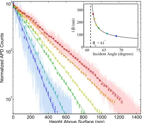
5.1.1 TIRM set-up . . . 50

5.1.2 Calibration curves with and without AR Coating . . . 52

5.1.3 Calibration curves relation to Debye length . . . 54

5.2.1 Calibration curves as a function of probe beam angle . . . 56

5.2.2 Measured and predicted near-wall hindered diffusion . . . 60

5.2.3 Potential energy profiles measured with 4 trap powers . . . 61

6.4.1 Experimental set-up: f N forces measurement . . . 68

6.4.2 Power spectral density (PSD) of a Brownian probe . . . 70

6.6.1 Force resolution of floating probe measurements . . . 71

6.6.2 Agreement between measurements and Mie theory . . . 72

6.7.1 Least-squares fit to MSD . . . 77

6.7.2 Spring constant of optical trap . . . 78

6.7.3 Numerical simulations confirming Mie theory approximation . . 88

7.2.1 Optically trapped sphere in its anisotropic environment . . . 94

7.3.1 Elliptical orbits of trapped microspheres, varying frequency . . . 96

7.3.2 Elliptical orbits of trapped microspheres, varying radius . . . 97

7.3.3 Measured and predicted torque applied to fluid . . . 99

7.4.1 Setup of 2D measurement . . . 102

7.4.2 Analysis flow for determination of unknown mechanical parameters 103 7.4.3 Power spectral density in 2D . . . 104

7.4.4 Damping coefficients perpendicular and parallel to wall . . . 105

7.4.5 Trap stiffness in the two directions . . . 107

7.4.6 Net force on an microparticle in elliptical orbit . . . 108

7.4.7 Optical forces in an evanescent field . . . 111

7.4.8 Angular momentum in microsphere undergoing elliptical motion 116 8.0.1 Force microscope in operation . . . 118

8.1.1 CAD Drawing of objective and prism assembly . . . 120

8.2.1 Optical paths and equipment on top level . . . 122

(10)

8.2.3 Photo of LED beam path . . . 125

8.2.4 Photo demonstrating how to find objective focus . . . 126

8.2.5 Dark-field microscope image of PS beads . . . 127

8.2.6 Photo showing capacitive sensor attachment . . . 128

8.2.7 Photo showing alignment of beam expander . . . 130

8.2.8 Photo of probe beam configuration . . . 132

8.2.9 Photo of confocal collection scheme . . . 133

8.2.10Photo of pump beam optics . . . 135

8.2.11Schematic of a QPD . . . 136

8.2.12Photo showing back-scattered trap beam . . . 137

8.2.13Photo of balanced detector and optics . . . 138

8.3.1 Photo showing fiber coupling alignment . . . 140

8.4.1 Microfluidic chamber . . . 142

8.4.2 Drawing of coverslip with laser drilled holes . . . 143

8.4.3 Drawing of sealant cut into shape . . . 143

8.4.4 Drawing of assembled microfluidic chamber . . . 144

8.4.5 Photo of microfluidic chamber . . . 145

8.5.1 Microscope image of pump beam spot . . . 146

(11)

(12)

Acknowledgments

The list includes my PI, of course, and Alex Woolf, Simon Kheifets, Vincent Ginis, Andrea Di Donato, Zhang Wu, Brandon Foley, and Arman Amirzhan. To my advisor and scientific collaborators: thank you for your contributions to this project. It was a joy to work with you.

There are also those who have been very helpful in their capacity as university staff. Stacia Zatsiorsky and Deni Peric, our lab’s administrators, Philippe de Rouffignac and Jason Tresback from the Center for Nanoscale Systems (CNS), are all very good at their jobs and deserve raises and promotions and more time off.

An even larger circle of colleagues and acquaintances have lent their help and their time out of sheer kindness. Some– Mikhail Kats, Sorel Massenburg, Tom Kodger, Max Eggersdorfer– taught me skills, some– David Siegel, Keith Karasek– offered advice. Thank you for your time; you’re examples to me.

(13)

So how, children, does the brain, which lives without a spark of light, build for us a world full of light?

Anthony Doerr

1

Light-Matter Interaction

To see the words on this page, to feel the sun on your skin, is to experience the interaction of light with matter. Light and matter are so present in our lives that, without study, most of us know quite a lot about these interactions. For instance, we know that trees cast shadows and these shadows are dark. We can’t see through lead but we can see through air. A mirror shows our reflection but not a piece of paper.

(14)

1.1 Why does light interact with matter?

Atoms are electrically neutral, but their parts are not. Apply a voltage, or electric field, to a conducting material and something happens – a current of electrons begins to flow.

For an insulating material, the change is more subtle. Nevertheless, electron clouds deform in response to the field and the loss of symmetry causes the atom to become slightly polarized.

A linear material is the simplest, most familiar type. As long as the field is small, the induced polarization per unit volume in these materials is proportional to the electric field. That is,

⃗_P _∝⃗_E _(1.1)

The constant of proportionality is determined by the electric susceptibility,χ_e, of the material– just how readily it polarizes compared to other materials under a certain applied field.

Lightis an oscillating, propagating, electromagnetic field. When it strikes a material, the atoms that compose it feel an electric field and a magnetic field, which are quickly changing in direction. Its response, or its electric susceptibility, depends on both the composition of the material and the frequency of oscillation of these fields.

The result of light striking matter is that light can be absorbed, confined, scattered, or even emitted.

(15)

Our skin, like most other parts of our body, is composed mainly of water. Water, a molecule with a permanent dipole, stretches and rotates in the presence of an electric field. Infrared light excites a number of these vibrationalmodes, so in effect, the energy of the photon is converted into kinetic, or thermal energy. It is because of absorption that sunlight feels hot on our skin.

In scattering, light encounters matter and is deflected from its original direction of travel. It may be redirected to travel in largely the same direction, a completely new direction, or in many directions at once. The difference in scattering phenomena explains the different visual experiences of looking through a piece of glass, seeing your reflection in a mirror, and staring at a blank piece of paper.

Multiple reflections or total internal reflection may cause photons to become ”trapped” for some time in a limited spatial region. Optical confinement can refer to waveguides or micro-cavities or even defects within a photonic crystal [36]. These effects, along with stimulated emission phenomena where the presence of a photon induces matter to emit more photons with the same wavelength and phase [20], are a bit outside of common intuition and experience. But they are nevertheless important for everyday technologies. For instance, stimulated emission is a key physical process in the workings of a laser, and fiber-optic cables which allow Internet communication are waveguides which confine and transmit light pulses over long distances with minimal loss.

1.2 Optical forces

The easiest way to understand how a force may arise from from light-matter interactions is to consider a single dipole,⃗_p_{. A dipole moment is formed by the}

spatial separation of a positive charge from an equal magnitude negative charge. Polarization refers to the creation of such a dipole moment in matter.

(16)

+ q

- q

[image:16.612.233.385.93.135.2]

d

Figure 1.2.1: Drawing of a dipole moment.

The dipole may be permanent, such as in the case of water molecules, or induced. Induced dipoles follow the relation in Equation 1.1 for linear materials, with⃗_p∝⃗_E_.

Consider such a dipole, for example Figure 1.2.1, whether it is permanent or induced, in an electric field.⃗Eis pointed in some direction which forms an angle

θwith⃗d. An electrostatic force will pull the positive charge in theEˆdirection and push the negative charge in the−Eˆdirection, which in general results in a torque,

τ, on the dipole.

⃗τ=⃗p×⃗E (1.3) This torque goes to zero when⃗dbecomes parallel to the electric field, so it can be intuitively understood that an electric field rotates the dipole to align with the field.

In this case, in a constant electric field, there is nonet forceon the dipole since the force on the negative charge is exactly equal and opposite to the force on the positive charge. If field strength varies from position to position, however, this is no longer the case. Consider a dipole which lies along the x-axis,

⃗_F_net₌⃗_F₊₊⃗_F₋₌_q(⃗_E₍_x₀₊_d₎₋⃗_E₍_x₀₎)

=qdd⃗E dx

x=x0

,

where, in the last line,dwas approximated to be very small. The result is the net force is proportional to the gradient of the electric field multiplied by the dipole moment. This can be generalized in three dimensions as

⃗_F

(17)

For an induced dipole, where⃗pis itself proportional to⃗E, the net force can be re-written, using a vector calculus identity for∇⃗(⃗A·⃗B), to be proportional to the gradient of the intensity of the electric field.

⃗_F

net =

1 2

⃗

∇(⃗p·⃗E) = 1

2α

⃗

∇E2 (1.5)

The above calculations provide a kind of crude intuition for what we will later call thegradient force. Another way of understanding this force is that the dipole tends to move into a configuration which wouldminimize energy.

Equation 1.5 shows that the net force may be written as a gradient of some quantity. This implies the force is conservative and that this quantity is the negative of a potential energy, where,

U=−1

2⃗p·⃗E=− 1 2αE

2 _(1.6)

The lowest energy configuration occurs when the dipole moment is aligned with the electric field in the region of highest field. A similar argument may be made for permanent dipoles. Since most materials are polarizable, this tendency to be attracted to electric field maxima would be exploited in the creation of optical tweezers.

1.3 Optical tweezers

In 1986, Arthur Ashkin and his colleagues at Bell Labs demonstrated the first working optical tweezer [8], composed of a single, focused laser beam, and capable of capturing and holding in place microparticles ranging from nanometers to microns in size.

(18)

[image:18.612.226.388.100.232.2]

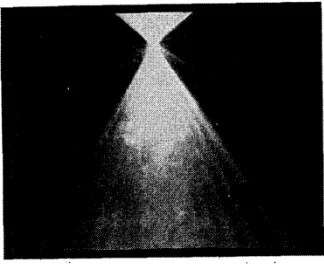
Figure 1.3.1: Ashkin’s 1986 microscope image of an optically trapped microsphere, showing, in the striations, the distinctive Mie scattering interference orders.

intensity region and the latter pushing the particle in the direction of light propagation. The physical explanation was given in two regimes. First, the dipolar regime was explored where the particle is approximated to be a point particle much smaller than the wavelength of light. Then, a ray optics picture was offered where the refraction of light by a particle much larger than its wavelength results in a change of momentum that causes an attractive force.

Though the explanations give a useful intuition, microparticles in general, including those used in the Ashkin experiment, fall into neither of the above categories [74]. The appropriate treatment is one using wave optics, but

accounting for the finite size of the scatterer. This approach, named Mie theory, is an exact scattering solution generally applicable to spherical particles interacting with an electromagnetic field.

1.4 Mie theory

(19)

z

x

y

IncidentField

[image:19.612.216.395.93.306.2]

ScatteredField

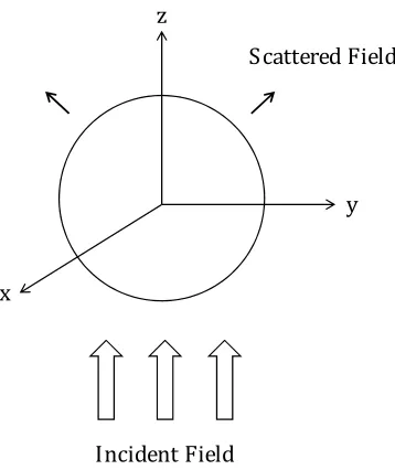
Figure 1.4.1: Mie scattering geometry showing spherical particle, incident and scat-tered fields.

In its simplest form, Mie theory imagines a plane wave incident on a sphere. The oscillating fields induce a polarization within the sphere which varies with time and position. Oscillating charges and dipoles radiate and a scattered field results, which propagates radially outward from the sphere. The superposition of the incident and scattered fields give the distinctive Mie scattering interference pattern in the far-field, visible in Figure 1.3.1.

The problem can be solved in three steps. First, obtain a set of generic solutions to Maxwell’s wave equations which form a complete orthonormal basis in the spherical coordinate system. Second, express the incident, scattered, and internal fields in terms of these solutions. Third, solve for the unknown

parameters in these fields by imposing boundary conditions derived from Maxwell’s Equations.

(20)

1.4.1 Step One: Vector spherical harmonics

The homogeneous wave equations for electric and magnetic fields in the absence of sources reads,

∇2_⃗_E₊_k2_⃗_E₌₀ _(1.7) ∇2_⃗

B+k2⃗B=0

wherek2 ₌_εμω2_{, and time-harmonic, monochromatic solution of the form}

⃗_E₌⃗_E

0(x,y,z)e−iωthave been inserted. Here,εandμindicate the optical

properties of the medium–εis theelectric permittivityandμthemagnetic permeability– andkis the wavevector in the medium.

Presented without derivation are theVector Spherical Harmonicsolutions which obey the vector wave equations in 1.7 as well as the individual Maxwell’s equations,

⃗

Ml,m =∇ ×⃗ (⃗rψ_l,m) (1.8)

⃗

Nl,m =

⃗

∇ ×_M⃗

l,m

k , (1.9)

with

ψ_l_,_m(r,θ,φ) = √

2

πZl(kr)P

m

l (cosθ)eimφ. (1.10)

In these equations, the indicesl,mare integers, withl≥0 and|m| ≤l. The functionZlrepresents aSpherical Bessel FunctionandPml are the set ofAssociated

Legendre Polynomials.

The solutions form a complete orthonormal set, and thus, any solution of the wave equation satisfying Maxwell’s Equations may be written as a linear

(21)

1.4.2 Step Two: Real fields as spherical harmonics

An operator,A, islinearif its action on a superposition of functions

(a1f1+a2f2+...) can be written as its action on each individual part such that,

A(a1f1+a2f2+...) = a1A(f1) +a2A(f2) +... (1.11)

whereaiare constants.

The linearity of Maxwell’s Equations allows separate solutions found for incident and scattered fields to be superimposed in each region of space. The total field, guaranteed to also be a solution to Maxwell’s Equations, is then connected across regions by boundary conditions.

Any electromagnetic field can theoretically be written in terms of the spherical harmonics discussed in the previous section.

⃗_E

inc =

∑

l,m

[

αl,m⃗Nl,m+β_l,mM⃗l,m

]

(1.12)

Since the incident field is known, the coefficientsαl,mandβ_l,mcan be

computed directly. The incoming magnetic field may be found by taking the curl of this expression, so no new coefficients are necessary to writeH⃗inc.

A similar expression can be written for the scattered field,Escatand the field

inside the particle,Eint.

⃗_E

scat =

∑

l,m

[

al,m⃗Nl,m+bl,mM⃗l,m

]

(1.13)

⃗_E

int=

∑

l,m

[

cl,m⃗Nl,m+dl,mM⃗l,m

]

(1.14)

SinceEincis often simply expressed in Cartesian coordinates, e.g. a

(22)

1.4.3 Step Three: Boundary conditions

Boundary conditions derived from Maxwell’s Equations govern the behavior of electromagnetic fields crossing from one medium into another. They are phrased in relation to the interface normal direction,ˆn, which, in the case of a sphere with its center at the coordinate origin, is theˆrdirection.

It becomes clear that complex manipulations of the previous sections have the purpose of simplifying this matching procedure. The total fields on the interior of the Mie particle are related to the total fields in the surrounding medium by

ˆr×(⃗Eout−⃗Ein) = 0 ˆr·(εout⃗Eout−εin⃗Ein) =0 (1.15)

ˆr×(μ_out⃗Bout−μ_in⃗Bin) = 0 ˆr·(⃗Bout−⃗Bin) = 0,

assuming no ”free” surface charges and currents exist.Incidentally, these boundary conditions also work for scatterers which are electrical conductors, as long as the free electron contribution to the polarization is included in a complex dielectric function,˜ε.

Replacing⃗Eout =⃗Escat+⃗Eincand⃗Ein =⃗Eint, and similarly for⃗B-fields, the

coefficients may be matched order by order resulting in exceptionally complex expressions fora,b,c, andd, which I will not quote here.

Two important points should be noted which will become important later on. First, the Mie scattering solution is an infinite series. Its convergence depends on a diminishing contribution from scattering at higher orders. It becomes necessary in a practical calculation to truncate the series at a certain order, given an acceptable margin of error. As the Mie particle becomes larger relative to the wavelength, contributions from higher orders grow in importance, thus, Mie theory calculations are limited in a practical sense.

(23)

discuss the framework for calculating optical forces from electromagnetic fields.

1.5 The Rayleigh approximation

Mie theory gives the generalized scattering solution for all particle sizes and all wavelengths of light. In the limit of small particles, however, the much simpler dipolar solution, as discussed in Section 1.2 may be recovered through an approximation.

Two criteria must be met. The particle radius must be much smaller than the wavelength of light (ka≪1), and the index of refraction of the scatterer must be close to that of the medium (ns/nm ≈1). In this case, the Mie infinite series may

be approximated by the first (dipolar) term, withl=1. For an incident, linearly polarized plane wave, all coefficients withm̸=1 are zero, and the only scattering coefficients to be considered area1,1andb1,1. This greatly simplifies the

calculations, and results in the familiar Rayleigh scattering cross-section which is proportional to the fourth power of the frequency of light,

σscat = 6π

k2

[

4(_ka)6

9

(ns/nm)2−1

(ns/nm)2+2

2] (1.16)

= k

4

6π|α|

2_,

whereαis the complex polarizability of the sphere, defined asα=3V_NN22₊−1₂.Vis

the volume of the sphere.

1.6 The Maxwell stress tensor

Electromagnetic waves carry momentum. When light is scattered by a particle, some portion of it is redirected from its original path, that is, its momentum is altered. The scatterer therefore feels a recoil force due to the conservation of momentum.

(24)

Recall that, in Section 1.1, we discussed the reason that light interacts with matter– matter is made up of positive and negative charges. Imagine one of these charges inside the scatterer, immersed in an electromagnetic field, perhaps the total field calculated in Section 1.4. Force on this charge, at a specific moment in time, given by the Lorentz force law, is

⃗_F₌_q₍⃗_E₊_⃗_v_×⃗_B₎_. _(1.17)

We could calculate the total force on the scatterer by finding the force on each individual charge, but it is often easier to work with fields. Using Maxwell’s Equations to replace the charge in Equation 1.17 with the fields produced by the presence of the charge, and integrating over all charges, the total force (in each direction) can be written [30],

Fi =

I

S

Tij·daj−εμ

d dt

∫

V

SidV, (1.18)

where

Tij≡ε

( EiEj−

1 2δijE

2)₊ 1

μ (

BiBj−

1 2δijB

2)

(1.19)

is the Minkowski form of theMaxwell Stress Tensor[38] ¹. The indicesi,jspan the three dimensions,δijis the Kronecker delta, and⃗Sis the Poynting vector of

the electromagnetic field. Using the relation between the Poynting vector and the momentum density of an EM field,⃗ϱ_em=⃗_S/_c2_{, Equation 1.20 may be rewritten,}

d

dt(Pmech,i+Pem,i) = I

S

Tij·daj (1.20)

whereFi= dP_dti has been used, andPmechandPemrepresent the total momentum

of the charges and fields, respectively, within the volume.

In this form, this equation is clearly an expression of conservation of

(25)

momentum. In words, the change in total momentum– of charges and fields– within a volume is equal to the rate of momentum ”flow” into that volume.

In a steady-state problem, the fields are unchanging, and_dtdPemmay be

neglected. So it can be interpreted that by reading the change in momentum of the EM field, one can infer the force on the scatterer within.

Generalized to time-averaged quantities of oscillating fields, as in the case of light whereEi(t) = ˜EieiωtandBi(t) = ˜Bieiωt, the Maxwell Stress tensor is, quite

similarly,

⟨Tij⟩=

1 2

[ ε

( ˜

EiE˜∗j −

1 2δij|E|

2)₊ 1

μ (

˜

BiB˜∗j −

1 2δij|B|

2)]

(1.21)

(26)

Repose is only an illusion due to the imperfection of our senses.

Jean Baptiste Perrin

2

Thermal Motion

When Jean Baptiste Perrin was, in 1926, awarded the Nobel Prize in Physics for his work on Brownian motion, the prize credited his discovery ofthe

discontinuous structure of matter. This is the lesser known story of the atom, but in fact, the prediction and measurement of thermal motion had settled a great debate.

The turn of the nineteenth century brought to physics a wave of new ideas. Classical thermodynamics, which had enjoyed much success in its energetic description of nature, met a new challenger in the form of molecular kinetic theory. That matter could be granular was not a brand new idea–chemists since John Dalton had been using the theoretical construct of atoms–but it was not believed to be any more than a mathematical tool.

(27)

and molecules and aimed to describe thermodynamics through their statistical, ensemble behavior. The first experimental validation of this theory, which finally put to rest the concept of continuous, infinitely divisible matter, came in 1909, and was a measurement of Brownian motion.

2.1 Perrin’s argument for atoms

Translated from Perrin’s 1909 paperBrownian Motion and Molecular Reality[56] is this thought experiment:

What is really strange and new in the Brownian movement is, precisely, that it never stops. At first that seems in contradiction to our every-day experience of friction. If for example, we pour a bucket of water into a tub, it seems natural that, after a short time, the motion possessed by the liquid mass disappears. Let us analyse further how this apparent equilibrium is arrived at: all the particles had at first velocities almost equal and parallel; this co-ordination is disturbed as soon as certain particles, striking the walls of the tub, recoil in different directions with changed speeds, to be soon deviated anew by their impacts with other portions of the liquid. So that, some instants after the fall, all parts of the water will be still in motion, but it is now necessary to consider quite a small portion of it, in order that the speeds of its different points may have about the same direction and value...

What we observe, in consequence, so long as we can distinguish anything, is not a cessation of the movements, but that they become more and more chaotic, that they distribute themselves in a fashion the more irregular the smaller the parts.

(28)

[image:28.612.218.396.96.243.2]

Figure 2.1.1: Sketch of Brownian motion from Perrin’s 1909 paper.

The results of his experiment–the observation of Brownian motion–is itself the answer to this question: no. He goes on to make a logical argument for discrete matter on this basis.

Since the distribution of motion in a fluid does not progress indefinitely, and is limited by a spontaneous re-co-ordination, it follows that the fluids are themselves composed of granules or molecules, which can assume all possible motions relative to one another, but in the interior of which dissemination of motion is impossible. If such molecules had no existence it is not apparent how there would be any limit to the de-co-ordination of motion...

The Brownian movement is permanent at constant temperature: that is an experimental fact. The motion of the molecules which it leads us to imagine is thus itself also permanent. If these molecules come into collision like billiard balls, it is necessary to add that they are perfectly elastic, and this expression can, indeed, be used to indicate that in the molecular collisions of a thermally isolated system the sum of the energies of motion remains definitely constant.

(29)

to suggest that every fluid is formed of elastic molecules, animated by a perpetual motion.

2.2 Einstein’s kinetic theory of Brownian motion

The success of Perrin’s 1909 experiment is largely the agreement of its quantitative results with a prediction made by Albert Einstein in 1905– and independently, by Marian Smoluchowski in 1906– based on molecular kinetic theory [19].

Einstein’s key insight was that a microscopic particle undergoing Brownian motion differed from a solute molecule dissolved in a liquid only by its dimensions. As such, a collection of Brownian particles would be expected to exhibit its own osmotic pressure.

By incorporating the mobility (μ= 1/γ) of these individual particles in calculating a drift current due to osmotic pressure, Einstein derived an expression for the diffusion coefficient,D, in Fick’s Laws, which had been previously left as an empirical quantity:

D=kBTμ (2.1)

or, if the particle could be approximated as a sphere,

D= kBT

6πηR (2.2)

wherekBis the Boltzmann constant,Tis the temperature in Kelvin,ηthe

viscosity of the fluid medium andRthe radius of the diffusing body.

Recognizing, also, that the key measurable quantity in Brownian motion is the mean-squared-displacement, rather than the velocity, Einstein derived the additional relation, for one-dimensional diffusion,

⟨Δx2⟩=₂_Dt, _(2.3)

(30)

proportional to the square-root of time. This distinctive feature of a random walk enabled the quantitative comparison of Perrin’s measurements with kinetic theory– the direct evidence needed to make the definitive case for the atom.

2.3 The Fluctuation-Dissipation Theorem

Einstein’s equation (2.1) happened to be an early example of a fluctuation-dissipation relation. However, the idea would not be formalized until 1928, when Harry Nyquist reviewed the problem of thermal fluctuations in conductors in electrical circuits [54]. Then, only in 1951, came the proof for the general form of the fluctuation-dissipation theorem, which unified the law in all linear systems which obey microscopic reversibility [15].

[image:30.612.217.399.387.530.2]

The fluctuation-dissipation theorem, as its name implies, finds a fundamental connection between thermal fluctuations of a physical system and the system’s dissipative qualities.

Figure 2.3.1: Sketch of brownian motion at a molecular level. [68]

(31)

due to collisions with these fluid molecules– tending to dissipate the energy of its motion and bring the particle to rest.

Since the two effects come from the same origin, it is not surprising that they are related. Or, in the language of Perrin’s argument in the earlier section, in a system that is reversible, re-coordination (fluctuation) is simply the inverse of de-coordination (dissipation), facilitated by the same physical processes (collisions).

Specifically, it can be shown [15] that the thermal force power spectrum,

SF =|˜Fth(ω)|2, of Brownian motion of a particle is proportional to its drag

coefficientγ. Thus, thermal noise increases with higher temperatures as well as more dissipation.

SF =2γkBT (2.4)

Similarly, the power spectrum of fluctuations in an electrical circuit is related to the resistance of the circuit to current flow¹.

2.4 Langevin equation of motion

2.4.1 Free motion

Though a particle undergoing Brownian motion moves in an essentially non-deterministic way, its motion can be accurately modeled using the familiar Newtonian dynamic equations. In the most simple case of unconstrained one-dimensional motion, the Langevin equation reads,

mdv(t)

dt =−γv(t) +Fth(t) (2.5)

whereFthis the stochastic thermal force, andv(t) = dx (t)

dt . The nature of a

stochastic force ensures that any given instance of this force at timetcannot be

¹The notion that a quantity proportional to the square of some variable would be called the

(32)

exactly known, however, statements can be made about its ensemble average values.

Since the particle is equally likely to be struck by a fluid molecule from either side, the average stochastic force should be zero. However, as explained in Section 2.3, the second moment of the distribution,⟨Fth(t)Fth(t′)⟩is non-zero

and related to the drag,γ, by Equation 2.4. Thus, it can be shown thatFthhas the

following properties:

⟨Fth(t)⟩=0 ⟨Fth(t)Fth(t′)⟩=2γkBTδ(t−t′). (2.6)

Here,⟨...⟩is used to denote the ensemble average, and the delta-function ensures that each impulse is uncorrelated with every other.

From this very simple model one can already deduce some universal aspects of a particle’s motion in fluid. Taking an average of Equation 2.5, and setting the mean stochastic force to its average value of zero, we obtain,

⟨v(t)⟩=⟨v(0)⟩e−mγt (2.7)

whereτp =m/γemerges as an important time scale which we will call the

momentum relaxation time. It can be understood as the time it takes for a particle to lose its ballistic momentum in the fluid. In other words, on time scales much longer thanτp, the particle behaves as if it has no inertial mass.

If we Fourier transform Equation 2.5 and rearrange to write the particle’s motion˜x(ω)in terms of the driving forceF˜th(ω), we obtain,

˜

x(ω) = ˜F(ω)

mω2₊_iγω (2.8)

and we may identify the complex quantityχ(ω) = _mω2₊1_iγωas theresponse functionof the linear system.

(33)

102 103 104 105 106 107 108 Frequency (rad/s)

10-35 10-30 10-25 10-20 10-15

Power Spectral Density (m

[image:33.612.187.412.103.272.2]

2/Hz)

Figure 2.4.1: Power spectral density of a free Brownian particle in fluid with typical parameters: γ=1×10−7_N*s/m,_k

BT=4×10−21 J,τp=10−6 s

particle’s position, recallSx(ω) =|˜x(ω)|2:

Sx(ω) =

SF(ω)

m2_ω4₊_γ2_ω2 =

SF

γ2_ω2₍ω2

ω2

p +1)

(2.9)

whereSF(ω) =2γkBTis a constant, as determined in the earlier discussion on

fluctuations and dissipation. Two distinct regimes emerge, again, defined by their relationship toτp =ω−p1. First, on very short time scales, orω≫ωp, the first

term in the denominator dominates, andSxis proportional toω−4. The motion is

ballistic. However, at time scales longer thanτp, whereω≪ωp, motion is

diffusive andSxis proportional toω−2. Figure 2.4.1 shows this dependence.

2.4.2 Constrained motion

(34)

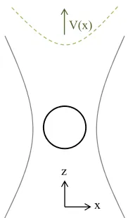
x z

[image:34.612.260.351.93.248.2]

V(x)

Figure 2.4.2: Schematic of an optically trapped microsphere. In green: an approxi-mation of the harmonic trap potential.

Equation 2.5 with a new term accounting for the trap’s restoring force,

md

2_x₍_t₎

dt2 =−κx−γ

dx(t)

dt +Fth(t) (2.10)

where the equation of motion is now expressed in terms of the position variable,

x(_t)_{, and}_κ_{represents the stiffness of the optical trap, or its}_{spring constant}_.

The complex response function becomes,

χ(_ω) = 1

κ−mω2₊_iγω (2.11)

resulting in a Lorentzian expression for the power spectral density,

Sx(ω) =

SF(ω)

m2

[ (ω2

0−ω2)2+ω2pω2

]. (2.12)

The natural resonanceω0of the system was introduced and defined as

ω20 =κ/m. Completing the square to put Equation 2.12 in a more familiar form,

Sx(ω) = SF

(_ω)

m2[₍_ω2−_ω2

L)2+ (21Γ)2

(35)

we find that the Lorentzian has a peak centered aroundωL =

√ ω2

0− 12ω2p, with a

width of Γ=2√ω4 0−ω4L.

First, let’s examine how the optical trap affects a typical microsphere in fluid. Figure 2.4.3 compares the power spectrum of the trapped sphere with that of the free sphere plotted in Figure 2.4.1.

10-2 100 102 104 106 108

Frequency (rad/s) 10-30

10-20 10-10

2/Hz)

Free motion Confined motion

Figure 2.4.3: Power spectral density of an optically trapped Brownian particle in fluid compared with that of a free particle. Typical parameters were used: γ=1×10−7 N*s/m,kBT=4×10−21 J,τp=10−6 s,κ=1×10−6 N/m.

One can see immediately that on short time scales– i.e. at high frequencies– the motion of an optically trapped sphere in indistinguishable from that of a freely diffusing sphere. Intuitively, on short time scales, the Brownian particle does not ”sense” the optical trap. On long time scales– at low frequencies– however, the motion is limited compared to that of a free particle. This can be understood as the optical trap imposing a sort of ”cap” on the maximum mean-squared displacement.

(36)

0 0.2 0.4 0.6 0.8 1 1.2 1.4 1.6 1.8 2 Normalized Frequency (w/w0)

0 0.5 1 1.5 2 2.5 3 3.5 4

2/Hz)

#10-15

Underdamped Critically damped Overdamped

Figure 2.4.4: Power spectral density of an optically trapped Brownian particle in fluid, showing different dynamic regimes. Fixed parameters: kBT =4×10−21 J,κ =

1×10−6_{N/m. Underdamped:} _ω

p=0.5ω0. Critically damped: ωp =ω0. Overdamped:

ωp=2ω0.

fixedω0.

The three regimes are labeledunderdamped,critically damped, andoverdamped

in analogy to the classic problem of a damped harmonic oscillator. A typical microsphere in a fluid environment corresponds to aωp ≈500ω0case, or a

highly overdamped case. On the other hand, the viscosity of air is 100 times smaller than that of water, and a critically damped or even underdamped regime may be reached.

Since all measurements described in this document were made in a fluidic environment, we can focus on the highly overdamped case. This specialization allows us to make a few simplifying approximations. First, recall thatτp =m/γ

defines the time scale for dissipation of inertia. Sinceτpis on the order of a

microsecond, instruments operating with sample rates on the order of kHz should be insensitive to the effect of particle mass. Testing this hypothesis, we eliminate the middle term in the denominator of Equation 2.11 to obtain,

χ(_ω) = 1

(37)

with a correspondingly simplified power spectrum,

Sx(ω) =

SF(ω)

γ2

[(

κ γ

)2

+ω2

]. (2.15)

we can identify the quantityκ/γas a corner frequency,ωc. At frequencies much

larger than the corner frequencyω≫ωc, the power spectrum is proportional to

ω−2. This is exactly the diffusive behavior discussed earlier. At frequencies much lower than the corner frequency, the power spectrum is a constant, and the motion is capped.

10-2 100 102 104 106 108

Frequency (rad/s)

10-35 10-30 10-25 10-20 10-15

2/Hz)

Exact power spectrum Approximation

Figure 2.4.5: Power spectral density of an optically trapped Brownian particle in fluid, low-mass approximation compared with exact solution. Typical parameters were used: γ=1×10−7 _N*s/m,_k

BT=4×10−21J, τp=10−6s,κ=1×10−6 N/m.

Figure 2.4.5 compares the exact power spectrum from Equation 2.12 with the low-mass approximation of Equation 2.15 for a typical spherical microparticle in fluid. The excellent agreement of the two expressions on time scales larger than the momentum relaxation time,τp, allows the use of the low-mass approximation

(38)

2.5 Mean-squared displacement

Though themean-squared displacement(MSD) and thepower spectral density

(PSD) may look very different, they contain the same information about the dynamics of the system.

To see this, recall the alternate definition of the power spectral density as defined as the Fourier transform of the auto-correlation function,

Gx(τ) =⟨x(t)x(t+τ)⟩,

Sx(ω) = √1

2π

∫ _∞

−∞Gx

(_τ)_e−iωτ_dτ _(2.16)

The connection between the MSD and the autocorrelation function is straight-forward to derive. If⟨x(t)⟩is zero, and settingt′ =t+τ,

⟨Δx(τ)2⟩=⟨(x(t′)−x(t))2⟩

=⟨x(t′)2⟩ −2⟨x(t′)x(t)⟩+⟨x(t)2⟩

=2Var(x)−2Gx(τ) (2.17)

Therefore, the mean-squared-displacement⟨Δx(τ)2⟩_{can be written in terms}

of the variance and power spectrum as,

⟨Δx(τ)2⟩=2Var(x)−2√1 2π

∫ _∞

−∞Sx

(ω)eiωτdω (2.18)

Though the MSD and PSD contain the same information, occasionally it is more convenient to use one form over another, especially in performing least-square fits.

2.6 Reynold’s number

(39)

in fluid dynamics is the ratio of inertial to viscous forces in the system, and as such, quantifies their relative importance.

Re=Rvρ/η (2.19)

Ris the dimension of the object moving with velocityvthrough fluid,ρandηare the density and viscosity of the fluid, respectively.

Our daily experience exemplifies a high Reynold’s number system. As an example, a human swimming in a pool of water will have a Reynold’s number of about 104. We might be surprised, therefore, to find that many of our physical intuitions do not carry over to low Reynold’s number systems such as the ones in this study.

Objects moving in a low Reynold’s number regime do not behave as if they have inertia [63]. An applied force induces almost instantaneous movement, and when the force stops, so does the motion.

There is no notion of ”stirring” in the usual sense, either. Any mixing of fluids or particles in a low Reynold’s number regime due to stirring can be ”unmixed” by simply reversing the direction of agitation.

Finally, as will become applicable later, propulsion, or inversely, pumping, in such systems is governed by a different set of principles. These are principles of symmetry. Since there is no sense in propelling forward by ”pushing” back on the fluid, propulsion is achieved only through configurational changes of a body that break time-reversal symmetry [63]. An example is given in Figure 2.6.1.

Figure 2.6.1: Example of a low Reynold’s number swimmer from Purcell’sLife at Low Reynold’s Number [63]

(40)

(41)

Go placidly amid the noise and the haste, and remember what peace there may be in silence.

Max Ehrmann.Desiderata

3

Understanding noise

In February of this year, the Laser Interferometer Gravitational Observatory (LIGO) announced the first direct observation of a gravitational wave, triggered by the merger of two black holes 1.3 billion light-years away. Within three months of the initial detection, another event was confirmed. The evidence that these events are plentiful in the universe, and that their signatures can be measured quantitatively, has ushered in a new field of gravitational wave astronomy.

LIGO saw its first light in 2002. For nearly a decade, no gravitational wave signal was detected. In 2010 the instruments were taken down for a four year construction period, consisting of both major and minor technological upgrades. The final difference? A factor of 10 improvement in sensitivity.

(42)

the first gravitational wave signal appeared. I tell this story to make two points clear:

• Understanding noise is essential to the successful design of an instrument.

• A small increase in sensitivity of our instruments can usher in whole new worlds of science.

3.1 What is noise?

A signal,S, with arbitrary units, corresponds to some physical quantity that we would like to detect in the lab. We use an instrument whichmeasures S, but not to its exact value. Instead, our instrument adds a quantity,N, to our signal, which varies in value each time the measurement is taken, such that the output,T, is,

T=S+N. (3.1)

Nhere stands for some kind of instrumental noise, pulled from a distribution. Say we measure the quantity,T, a number of times. We would obtain a vector,Ti,

which is in each case equal toSi+Ni. But sinceSiis the same in each

measurement,Ti =S+Ni. Now we can derive some relevant quantities. First,

taking the average,

⟨T⟩=_S+⟨_N⟩. _(3.2)

We find that the average of the measured values,T, should be equal toSas long as the average noise,⟨N⟩is zero.⟨N⟩is also thefirst momentof its distribution. Squaring Equation 3.2 and then taking the average, we obtain an equation for the second moment ofT,

(43)

If each instance of the noise is uncorrelated with other instances, then

⟨NiNj⟩=⟨N2⟩δij, and, assuming that⟨N⟩is zero as before, Equation 3.3

simplifies to,

⟨T2⟩=S2+⟨N2⟩, (3.4) where⟨N2⟩_{is the}_{second moment}_{of the distribution, or its}_variance_{. Therefore, the}

variance ofT, defined as Var(T) = ⟨(T− ⟨T⟩)2⟩_is,

⟨(T− ⟨T⟩)2⟩=⟨T2⟩ −S2=⟨N2⟩. (3.5)

Figure 3.1.1: Sketch of a Gaussian distribution (Wikipedia Creative Commons).

We see thatTis drawn from a distribution as well, but one with a mean of the true signalS, and a variance of the noiseN. This is what is meant by the

uncertaintyon a single measurementTi. We can denote the uncertainty in the

same units asSby taking a square-root.

σT =

√

⟨(_T− ⟨_T⟩)2⟩₌√⟨_N2⟩ _(3.6)

(44)

measurement ofT. This quantity can be understood probabilistically. Typically, noise is Gaussian distributed¹, and for a Gaussian function, as pictured in Figure 3.1.1, two-thirds of the area is bounded by±σ. This means,for a single measurement T, there is roughly a 2/3 chance it will fall within σTof S, its true value.

3.2 Propagation of error

We’ve seen a simple linear example in Equation 3.6 of how errors propagate from variables to a function of such variables. To generalize, assume a linear function,

f(_x₁,_x₂, ..._x_n)_{, such that}

f(_x₁,_x₂, ..._x_n) =_a₁_x₁+_a₂_x₂+..._a_n_x_n. _(3.7)

If each variablexihas uncertaintyσi=

√

⟨x2

i⟩, to findσfwe need to begin by

squaring Equation 3.7. We can write the result in matrix form,

f2 =a21x21 +...a2nx2n+2a1a2x1x2+...2a1anx1xn...=Aijxixj, (3.8)

where summation over repeated indices is implied andAij =aiaj. To find the

uncertaintyσf=

√

⟨f2⟩_{, we take the average of both sides of the equation, and}

setting the general covariance,⟨xixj⟩=σ2ij, we obtain,

σ2f =⟨f2⟩=Aijσ2ij. (3.9)

In the simple case where all variables{xi}are uncorrelated with one another, the

propagation of error formula reduces simply to,

σ2_f =a2_iσ2_i. (3.10) This method of propagating error applies to general functionsf(x1,x2, ...xn)

(45)

which are not linear function of{xi}as well. The most common method utilizes

theTaylor seriesto rewrite the functionf({xi})as a sum of polynomials. Using a

Taylor expansion aroundx=μ, whereμis the mean ofx,

f(x) =f(μ) +f′(μ)x+f

′′₍_μ₎

2 x

2₊_... _(3.11)

Therefore, an arbitrary function of multiple variablesf(x1,x2, ...xn), to first order

in the Taylor series, may be written

f(x1,x2, ...xn) =

∂f

∂x1

μ₁

x1+

∂f

∂x2

μ₂

x2+...

∂f

∂xn

μ_n

xn+C. (3.12)

The same matrixAijas above may be written now withAij= _∂∂_xf_i|μ_i_∂∂_xf_j|μ_jand

the general formula for error propagation which results, assuming uncorrelated variables{xi}is,

σ2_f = (

∂f

∂x1

μ₁

)2

σ2₁ + (

∂f

∂x2

μ₂

)2

σ2₂+...

(

∂f

∂xn

μ_n

)2

σ2_n (3.13)

3.3 Turning down the noise

One nearly universal way of reducing the uncertainty of a measurement is to repeat that measurement many times. In a survey, this means increasing the sample size. In a camera, this means leaving the shutter open for longer. In the hypothetical measurement made in Section 3.1, we can take the average of the vector of independent measurements,Ti.

The error on themeanofT, orσ⟨T⟩, can be calculated from the error

propagation formula. Since,

⟨T⟩= 1

n ∑

i

Ti =

1

(46)

therefore,

σ2_⟨_T_⟩ = 1

n2

(

σ2_T₁ +σ2_T₂ +...σ2_T_n)= 1

n2(nσ 2

T) (3.15)

The error on the mean ofnmeasurements is smaller than the error on each individual measurement by the square-root ofn. That is,σ⟨T⟩ =σT/

√

n. To generalize this concept, we identify a signal’s average value,⟨T⟩, with its Fourier transform at zero frequency, where the discrete Fourier transform is defined,

˜

Tk =

1

n ∑

m

Tme2πikm/n. (3.16)

Thek=_{0 Fourier component is also known as the}_{DC component}_{of the}

signal. The same uncertainty can be assigned to any other Fourier component, that is, other values ofk, as long as the length of the signal is fixed.

w1

PSD

w2

Figure 3.3.1: The RMS noise is the square-root of the total power in a band,Ω, found by integrating the power spectral density (PSD) of noise betweenω1 andω2.

(47)

as defined by Equation 2.16. We can rewrite,

Gx(τ) =

1

√

2π

∫ _∞

−∞Sx

(ω)eiωτdω, (3.17) whereGx(τ) =⟨x(t)x(t+τ)⟩is the auto-correlation function of some noise

variablex(_t)_{. Setting}_τ=_{0, the equation above becomes,}

⟨x(t)2⟩= √1

2π

∫ _∞

−∞Sx

(ω)dω. (3.18) This is a statement that the total variance of the signal is equal to the integral over the entire power spectrum. The above can also be found through an application ofParseval’s Theorem, which posits the unitarity of a Fourier transform.

Consequently, the variance in a limitedband, with bandwidth Ω=ω2−ω1,

can be found by a finite integral of the power spectrum betweenω1andω2,

⟨x(t)2⟩_Ω = √

2

π ∫ ω2

ω1

Sx(ω)dω, (3.19)

whereSxis now the single-sided power spectral density. This calculation is shown

graphically in Figure 3.3.1. In the discrete case, this becomes,

σ2Ω =2

∑

ω1<ωi<ω2

Sx(ωi)Δω, (3.20)

where Δωis the minimum possible bandwidth defined by Δω = 2π

n, withnbeing

the total number of data points.It becomes clear in this form that the lowest RMS noise which can be achieved coincides with this minimum bandwidth and a choice of ω0such that Sxis also minimal.

σ2_min=2Sx(ω0)Δω (3.21)

(48)

more,

σmin=

√

4πSx(ω0)

n . (3.22)

A technique calledlock-in detection, which will be utilized in this work, enables measurement in this specified, optimized band. By modulating a weak signal at the the frequencyω0, and performing a single point Fourier transform, maximum

(49)

There’s plenty of room at the bottom.

Richard Feynman

4

Force Microscopy

For the different orders of magnitude forces in our lives there exist very different methods of measurement. For instance, a bathroom scale, using a spring or a strain gauge, is useful in the range of tens to hundreds of newtons. For larger forces a piezoelectric or hydraulic system may be more ideal, and can be

employed, for instance, in a truck weighing station. For very small forces, such as the forces which cause proteins to fold in a particular way, a common approach is to track the mechanical deformation of a compliant probe.

(50)

motion of the trapped particle relative to its equilibrium position is indicative of a mechanical force. Though AFM’s are the standard for performing scanning probe measurements, floating probes have several important advantages including, most importantly, a much lower fundamental limit to the smallest force detectable.

4.1 Why measure femtonewton forces?

Measurements are scientists’ connection to reality. Not only do high precision instruments enable the validation of existing scientific theories, just as

[image:50.612.252.361.330.438.2]

importantly, they inspire the search for new theories and new models. It is therefore difficult to predict the kind of impact a two-orders-of-magnitude improvement in force sensitivity will have in various scientific fields.

Figure 4.1.1: The formation of DNA loops, shown here, is believed to be regulated by femtonewton forces. Graphic from Hfsp.org.

Biology.An important point of comparison in biological systems iskBT, or the

energy scale of thermal fluctuations. For physical systems in a thermal bath, interaction with energies much smaller thankBTwill tend to have a depressed

(51)

However, recently scientists have begun to consider the effects of femtonewton forces in biology, specifically the important roles they may play in biomolecule morphology and structure, the formation of DNA loops and, consequently, in gene regulation [1,5,12,17].

Optics.Richard Feynman once said about the future of physics, ”There is plenty of room at the bottom.” And indeed, recent decades have seen a boom in nanoscale research and fabrication. A particularly interesting area of research focuses on the fabrication of nano- and micro-scale mechanical devices and sensors– miniature pumps, probes, and switches– for use in, among other applications, lab-on-a-chip systems [29]. Light has emerged as a natural tool for the control of individual nano-scale components, with ability to non-invasively manipulate each part individually, as well as many parts in parallel.

For all we know about light, physicists are still developing intuition for the myriad of effects of light on matter. Ongoing studies exploring ”anomalous” forces involving tractor beams [52], spin-momentum locking in evanescent waves [11], and spin-orbital momentum transfer [78] have attracted much interest in recent years. They present potentially novel methods of actuation in microfluidic and miniaturized systems.

Since optical forces tend to scale withL2_{, where}_L_{is the probe dimension,}

while the inertia scales withL3_{, an efficient probe which responds mechanically}

to an optical force is destined to be small. In fact, they are typically optimized for

L≈λ, whereλis the wavelength of light. Spherical particles fitting this description, whose geometry enables exact calculation of optical forces via analytical Mie Theory (see Section 1.4), are precisely subject to forces at and below the limit of current instrument sensitivities.

4.2 Atomic Force Microscope

AFM cantilevers (see Figure 4.2.1) have the dimensions of a long

(52)

nanometers at the point.

Figure 4.2.1: Scanning Electron Microscope (SEM) image of an AFM cantilever tip.

The cantilever is attached to a piezo stage with freedom to move in all three dimensions. The vertical degree of freedom allows the acquisition of force curves as a function of height. The lateral degrees of freedom enables area scanning of a surface–revealing its various topographical and even chemical features. When the tip is brought close to a surface, interaction with the surface causes the cantilever to flex. The amount of flexure is measured by the displacement of a collimated laser beam specularly reflected from the back of the cantilever, as illustrated in Figure 4.2.2.

Force curves as a function of height,Fz(z), can be acquired as in the above

set-up by scanning the cantilever position with the piezo stage. At each height, the deflection of the cantilever is measured and converted into a force assuming the cantilever behaves as a spring, such that,

Fz =−κΔz (4.1)

(53)

Δ z QPD

AFM Cantileve r

Figure 4.2.2: Cantilever of an atomic force microscope (AFM), showing a quad-rant photodiode (QPD) detection method. In this example, a microsphere is shown attached to the cantilever tip and tethered by a protein to a functionalized surface. This is a typical method for measuring the forces needed to unfold a protein in a multi-step process.

restoring force is linear with deflection is only valid for small deflections. Thus, an AFM is sensitive to a certain range of forces, defined by the mechanical

properties of the chosen cantilever.

The smallest force measurable by an AFM is determined by the random noise in the system. We can define the force sensitivity of a system as the signal threshold which equals the system noise– for a signal-to-noise ratio of 1, or

S/N=1.

Noise breaks down into two main categories– measurement noise and thermal mechanical noise.

Measurement noise is inherent to the instrument and its various components in the signal path. It limits the precision with which an AFM cantilever’s position may be determined by the measurement apparatus. It, for instance, includes shot noise from the laser, electronic noise in the analog-to-digital converter, dark currents in our photodiode, and noise due to interference and resistances in the electronic circuits [53].

(54)

displacement.

Thermal mechanical noise, on the other hand, refers to actual random motion of the cantilever itself. The cantilever, in a thermal bath of fluid molecules, undergoes Brownian motion as a result of random collisions. We learned from Chapter 2 that the force spectrum of such collisions is flat– that is, the noise is

white– and the magnitude of these fluctuations is proportional to the temperature as well as the cantilever’s drag coefficient,γ.

To reiterate,

SF =2γkBT (4.2)

Since thermal mechanical noise results in physical displacements of the cantilever which may mask its response to an applied force, it imposes a fundamental limit on the sensitivity of any mechanical probe instrument. And this limit is much quicker reached in fluid than in air, on account of the orders of magnitude larger drag forces in the former environment. The result is the reduced functionality of AFM’s in fluid, un-helped by more compliant cantilever designs, and a limit to the achievable force resolution of around 1-10 piconewtons.

4.3 Floating Probe Microscope

To improve upon this fundamental sensitivity limit, some have proposed and fabricated miniature cantilevers [70] which present a reduced footprint in fluid. These cantilevers can be about ten-times smaller than those commercially available, and can hypothetically result in nearly an order of magnitude reduction in thermal noise and increase in sensitivity. But in trade, cantilevers become stiffer as they become smaller. Accordingly, they also scatter less light and are more difficult to track using the back-reflected laser beam. These increases in measurement noise have the potential to offset reductions in thermal noise.

(55)

independent choice of probe dimensions and trap stiffness, and microspheres as small as a micron in diameter can be used, resulting, potentially, in a more than two-orders-of-magnitude reduction in drag compared with commercial AFM cantilevers.

[image:55.612.258.350.186.318.2]

x z

Figure 4.3.1: Schematic of an optical tweezer. By moving the focus of the optical trap, the floating probe’s mean position can be manipulated to ”scan” across an area or volume.

Additionally, floating probe microscopes have the following advantages over conventional AFMs:

• An optical trap spring constant which is tunable by changing laser power.

• Non-intrusive and in situ contact-free measurements.

• Minimal mechanical coupling to noisy environment. In contrast with AFMs, noise shielding is generally unnecessary.

• Symmetric probe with three-dimensional force sensitivity, unlike AFM’s which are only able to measure forces in the vertical direction.