Volatiles in Protoplanetary Disks

Thesis by

Ke Zhang

In Partial Fulfillment of the Requirements for the Degree of

Doctor of Philosophy

California Institute of Technology Pasadena, California

2015

c

Acknowledgements

First and foremost, I would like to thank my advisor, Geoffrey Blake, for his patience, guidance, support, and inspiration that made this thesis possible. In retrospect, I am so grateful to have chosen Geoff as my mentor. He is a very special kind of advisor, so rare in the fast-paced world, who can be incredibly patient, waiting for a student to find her passion. But once the student has made up her mind, and starts to ask for resources, opportunities, and attention, he is so supportive and resourceful that the only limitation for the student is herself. It was a great privilege working with Geoff, who is ingeniously creative and vastly knowledgeable. Thank you for all the lessons, support, and, most importantly, for believing in and encouraging me.

I’m also thankful for John Carpenter who opened for me the wonderful door of (sub)mm-wave interferometry and gave me a very first opportunity to work with ALMA data. John, you are my role model as a rigorous scientist who understands his field profoundly and is dedicated to getting things right. I would also like to thank Colette Salyk for being such a great mentor and a supportive friend during my years in graduate school. Thanks for taking me to the summit of Mauna Kea and beautiful Charlottesville.

effort in my development as an independent scholar.

I thank my fellow graduate students for enriching my life at Caltech immeasurably. I’m thankful for students in the Blake group: Alex Lockwood, Masha Kleshcheva, Katie Kaufman, Danielle Piskorz, Dana Anderson, Brett McGuire, Brandon Carroll, Ian Finneran, and Marco Allodi. It was a great pleasure to work with you all and be your friend. Your company and laugher have turned many long nights in the remote observing room into fun and interesting times together. I’m grateful to my great class mates Kunal Mooley and Matt Schenker. Thank you for all the fun times in our first-year office, which made the stressful first-year transition into graduate school far more manageable. This was made all the easier thanks to the great atmosphere among the graduate students in both the Astronomy and Planetary Science options. Thank you all, especially Laura P´erez, Shriharsh Tendulkar, Ryan Trainor, Swarnima Manohar, Jackie Villadsen, Sebastian Pineda, Gwen Rudie, Allison Strom, Xi Zhang, Miki Nakajima, Chen Li, Zhan Su, Qiong Zhang, and Da Yang. A special thank you goes to Xuan Zhang, my best friend at Caltech, for very many happy lunches together and for sharing happiness, sorrow, and a belief in life and its joys.

Abstract

Planets are assembled from the gas, dust, and ice in the accretion disks that encircle young stars. Ices of chemical compounds with low condensation temperatures (<200 K), the so-calledvolatiles, dominate the solid mass reservoir from which planetesimals are formed and are thus available to build the protoplanetary cores of gas/ice giant planets. It has long been thought that the regions near the condensation fronts of volatiles are preferential birth sites of planets. Moreover, the main volatiles in disks are also the main C-and O-containing species in (exo)planetary atmospheres. Understanding the distribution of volatiles in disks and their role in planet-formation processes is therefore of great interest.

This thesis addresses two fundamental questions concerning the nature of volatiles in planet-forming disks: (1) how are volatiles distributed throughout a disk, and (2) how can we use volatiles to probe planet-forming processes in disks? We tackle the first question in two complementary ways. We have developed a novel super-resolution method to constrain the radial distribution of volatiles throughout a disk by combining multi-wavelength spectra. Thanks to the ordered velocity and temperature profiles in disks, we find that detailed constraints can be derived even with spatially and spectrally unresolved data – provided a wide range of energy levels are sampled. We also employ high-spatial resolution interferometric images at (sub)mm frequencies using the Atacama Large Millimeter Array (ALMA) to directly measure the radial distribution of volatiles.

Contents

Acknowledgements iii

Abstract v

1 Introduction 1

1.0.1 Protoplanetary disks . . . 2

1.0.2 Volatiles in planet formation . . . 6

1.0.3 Observations of volatile in prototplanetary disks . . . 8

1.0.4 Thesis Outline . . . 8

2 Evidence for a Snow Line Beyond the Transitional Radius in the TW Hya Protoplanetary Disk 11 2.1 Abstract . . . 12

2.2 Introduction . . . 13

2.3 Data reduction . . . 16

2.4 The TW Hya disk structure . . . 17

2.4.1 The dust temperature and density structure . . . 19

2.4.2 The gas density and temperature . . . 21

2.5 Retrieving the radial water vapor profile . . . 25

2.5.1 The water line model . . . 25

2.5.2 Best-fitting model . . . 28

2.5.2.1 The inner disk . . . 28

2.5.2.2 The transition region and the snow line . . . 32

2.6 Discussion . . . 34

2.6.1 The origin of the surface water vapor . . . 35

2.6.2 The water vapor abundance distribution in transitional disks . 37 2.6.3 Molecular mapping with multi-wavelength spectra . . . 39

2.7 Conclusions . . . 43

3 Comparison of the dust and gas radial structure in the transition disk [PZ99] J160421.7-213028 44 3.1 Abstract . . . 45

3.2 Introduction . . . 46

3.3 Observations . . . 48

3.4 Results . . . 49

3.5 Modeling Analysis . . . 51

3.5.1 Dust emission: model description . . . 52

3.5.2 Dust emission: fitting procedure and results . . . 53

3.5.3 CO emission: model description . . . 57

3.5.4 CO emission: fitting procedure and results . . . 58

3.5.5 Uncertainties from the choice of γ . . . 59

3.6 Discussion . . . 60

3.6.1 Comparing J1604-2130 with other transition disks . . . 60

3.6.2 Formation of the J1604-2130 transition disk . . . 61

3.6.3 Pressure trap and evolution . . . 64

3.6.4 Dust inside the cavity . . . 65

3.6.5 Outer disk radius . . . 65

3.7 Summary . . . 66

3.8 Acknowledgments . . . 67

4 Dimming and CO absorption toward the AA Tau protoplanetary disk: An infalling flow caused by disk instability? 75 4.1 Abstract . . . 76

4.3 Observations . . . 78

4.4 Results . . . 80

4.4.1 The physical properties of the absorbing gas . . . 81

4.5 The origin of the absorbing gas . . . 84

4.6 Acknowledgments . . . 88

5 Evidence of fast pebble growth near condensation fronts in the HL Tau protoplanetary disk 93 5.1 Abstract . . . 94

5.2 Introduction . . . 95

5.3 Observations . . . 96

5.4 Charactering the emission dips . . . 97

5.5 Condensation fronts of major volatiles in protoplanetary disks . . . . 98

5.6 Dust properties inside the dips . . . 101

5.7 Discussion . . . 104

5.8 Acknowledgement . . . 105

6 Conclusions and Future Directions 109 6.1 Summary of this thesis . . . 109

6.2 Future directions . . . 111

6.2.1 Opportunities from ALMA . . . 111

List of Figures

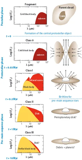
1.1 The current theoretical framework for the formation of a low-mass star

such as the Sun . . . 3

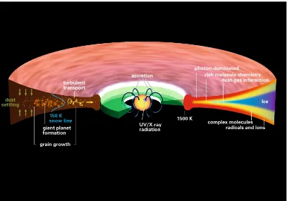
1.2 Physical and chemical structure of a protoplanetary disk . . . 5

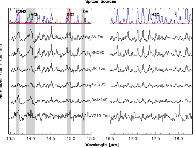
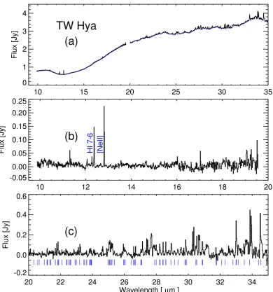
1.3 Spitzer IRS data on volatile molecule emission in protoplanetary disks 9 2.1 The Spitzer IRS spectrum of TW Hya . . . 18

2.2 SED fit and disk structure of TW Hya . . . 20

2.3 Model CO rovibrational fluxes of the TW Hya disk . . . 23

2.4 The best-fit radial abundance of water vapor in TW Hya . . . 29

2.5 Detailed comparisons of the Spitzer IRS spectrumwith RADLite LTE water models . . . 30

2.6 The sensitivity of selected water line fluxes to variations in the water vapor column density distribution . . . 31

2.7 Constraints on the sharpness of the snow-line in TW Hya . . . 34

2.8 The χ2 surface for LTE slab model water fits for TW Hya as a function of N and T . . . 37

2.9 The radial and vertical locations bounding water vapor emission from the TW Hya disk . . . 42

3.1 880 µm continuum map of J1604-2130 . . . 68

3.2 ALMA observations of CO J = 3-2 emission from J1604-2130 . . . 69

3.3 Dust surface density model of J1604-2130 . . . 70

3.5 Comparison of the ALMA 880 µm continuum image with the synthetic

model . . . 72

3.6 CO model for J1604-2130 . . . 72

3.7 Models with different γ . . . 73

3.8 ComparingJ1604-2130 with other transition disks . . . 74

4.1 V-band photometry time series of AA Tau . . . 89

4.2 COM-band spectra of AA Tau before and after the 2011V-band dimming 90 4.3 Time variation in the low-J 12CO and 13CO line shape(s) . . . 91

4.4 Model of the 12_{CO and} 13_{CO absorption components in January 2013 . 92} 5.1 Normalized radial surface brightness distributions of HL Tau at 0.87 (blue), 1.3 (red), and 2.9 mm (black) . . . 106

5.2 The expected condensation fronts in the disk mid-plane of HL Tau . . 107

5.3 Crosscuts of the spectral index in the HL Tau disk . . . 108

List of Tables

2.1 Disk parameters for the dust model . . . 21

2.2 Observed and calculated water line fluxes . . . 27

2.3 Volatile line tracers at different disk radii . . . 42

3.1 Disk parameters . . . 56

3.2 Continuum model parameters for different γ . . . 60

4.1 AA Tau Observation Log . . . 80

5.1 Parameters of the dips, normalized to the local continuum . . . 98

Chapter 1

Introduction

How did we get here? Are we alone in the Universe? Humankind has been seeking answers to these two enduring questions since ancient times. The answers to both questions demand an understanding of the formation of our own Solar system as well as the planetary systems around other stars.

We are privileged to be at a juncture where giant steps forward are being made in our understanding of planet formation. Over the past decade, more than three thousand planet candidates around other stars have been identified, indicating planet formation is a ubiquitous process in the local Universe. It is, however, striking to have discovered that most of the planetary systems around nearby stars show properties wholly distinct from our Solar system. What drives the large diversity observed? Might there be life in other planetary systems that are clearly so different from our own? There are two principal approaches to be taken in seeking further answers. One avenue involves the study of mature planetary systems around other stars, much as we have been doing for the Solar system. The architecture and chemical composition of a planetary system provides rich information on how it was formed. On the other hand, since planet formation is ubiquitous, we can also take advantage of nearby forming planetary systems to characterize the birth environments of planets directly, and use our knowledge of physics and chemistry to decipher the ongoing processes of planet formation.

disks largely regulates the final outcome of planetary system formation. Over the past decade, significant advances have been made in characterizing many basic properties of these disks, including the dust mass in disks and the disk evolutionary timescale(s). One of the most basic properties of disks, that of its chemical composition, is still largely unknown, however. Indeed, a rocky planet at the ‘right’ orbital distance may not be a habitable one, because it also must retain sufficient liquid water and critical elements such as carbon and nitrogen to form life.

Thus, we want to know the distribution of essential living-giving materials, or volatiles, such as water, CO/CO2 and NH3, in disks, before planetary surfaces are assembled. In particular, this thesis will focus recent steps toward understanding the distribution of volatiles in planet-forming disks, and seeks to answer questions such as: how are volatiles distributed in the disks? How does the general evolution of disks change their distribution? This brief introductory chapter is organized as follows: protoplanetary disks, in the context of star and planet formation, are defined and discussed in Section 1.0.1. I then introduce the definition of volatiles and discuss the important role that they play in planet formation processes in Section 1.0.2. I next describe current observations of volatiles in disks (Section 1.0.3), and conclude with an outline of the main chapters in this thesis.

1.0.1

Protoplanetary disks

3

?

t = 0 Formation of the central protostellar object

Birthline for pre–main sequence stars

Protoplanetary disk?

Debris + planets?

SN 0 2 4 6 8 10 12 14 16 18 0 10–2 10–1 101 103 105 107

100 ₁₀2 ₁₀4

5 10 15 20 25 30 35 40 45

0.0 0.1 0.2 0.3 0.4 0.5 0 1 Disk?

10 102

5 10 15

0 0.1 0.2 0.3 0.4 0.5

0 20 40 60 80 100 120

27_Al/24_Mg 27_Al/24_Mg 27_Al/24_Mg 27_Al/24_Mg

Melting of planet esimals

Nebula earliest c ondensat

es

Galactic backg round

δ

26Mg* (‰)

δ

26Mg* (‰)

δ

26Mg* (‰)

δ

26Mg* (‰)

Chondrules Pr es te lla r p ha se Pr ot os te lla r p ha se Pr e–main sequenc e phase

t < 0.03 Myr

t≈ 0.2 Myr

t≈1 Myr

t≈ 10 Myr

t = 0 Myr

t = 1–4 Myr

t = 1–5 Myr

λ(μm) Class III Lo g( λ Fλ ) Lo g( λ Fλ ) Fragment 1 Disk

10 102 λ(μm) Class II Lo g( λ Fλ ) Lo g( λ Fλ ) Lo g( λ Fλ ) 1 Black body Cold black body

submm

Infrared excess

10 10

102

1 10 102 ₁₀3

λ(μm) λ(μm) λ(μm)

Class I Class 0 Cold black body

submm

1 10 102 ₁₀3

Stellar black body

Core Parent cloud

a

b

c

d

356 Dauphas

·

The earliest stages of cloud collapse is represented by the so-called Class 0 objects – systems so deeply embedded within optically thick gas and dust that they are not visible even in deep near-IR rimages. At this stage, a rotationally supported disk may have been formed, but high angular resolutions observations are still sufficiently rare that our characterization the properties of the disks in this stage is poor. Unlike Class 0 objects, a rotational signature of a disk can easily be detected in Class I objects, which still have an envelope of infalling material, and which are usually associated with strong outflows or jets. The transition from a Class 0 to Class I object takes less than 0.5 Myr (Evans et al., 2009). As accretion proceeds, the envelope eventually dissipates (∼1 Myr) and the central young star becomes optically visible, representing the start of the Class II phase. For low and medium mass stars(_.3M), the gas disk is called a protoplanetary disk (Figure 1.2). These disks can last for a few million years (e.g., Haisch et al. 2001, Damjanov et al. 2007, Gutermuth et al. 2008), setting a critical limit for the timescale of the formation of gas giant planets. Once the gas disk has dissipated, the accretion onto the central star wanes and the flux excess at long-wavelengths decreases. A dusty debris disk of so-called ‘second generation’ dust (and small amounts of gas) can be formed via collisions between planetesimals (Class III).

1.0.2

Volatiles in planet formation

Volatiles are compounds with low sublimation temperatures (<200 K). In protoplan-etary disks, these are usually small molecules that form the principle reservoirs of the abundant elements carbon, nitrogen, and oxygen. The most important examples include water, CO, and N2/NH3.

Volatiles, especially water, play an essential role in planet formation. They not only provide the major solid mass reservoir for planetesimal and planet formation at sufficiently low temperatures, but also set the initial chemical composition in the atmospheres of forming planets.

Recent studies have also suggested that volatiles can greatly accelerate the forma-tion of planetesimals, from which planets are built. Planetesimals are usually defined as solid bodies that are held together by self-gravity rather than material strength (minimum size 100-1000 meters, Benz 2000). The growth from (sub)micron-sized ISM grains to planetesimals is a difficult process in protoplanetary disks, because once the grains grow into millimeter or larger size, the strong gas drag in a disk will cause solid bodies to collide destructively or they are dragged radially into the central star before they can grow into planetesimals. Volatiles can accelerate the growth process primarily via two routes: (i) condensed volatiles can add a large amount of solid material that is available for planetesimal formation; and (ii) the icy mantle formed by condensed volatiles on dust grains can greatly enhance their ‘stickiness’ in binary collisions.

The initial distribution of volatiles in a protoplanetary disk thus determines the chemical composition of planetesimals, which will later contribute to the bulk chem-ical composition of planets. Asteroids, meteorites and comets are believed to be the remnants of Solar system planetesimals that are either primitive or have that un-dergone dynamical and chemical processes. Nevertheless, these objects are our best window into the volatile composition of the Solar protoplanetary disk.

cores. In our Solar system, the terrestrial planets are all in the inner region while the gas and ice giants are located at further distances from the Sun. This architecture is attributed to the dividing line provided by the water condensation front, orsnow line, where most of the locally available water vapor condenses as solid ice. The condensed water ice can directly increase the surface density of solids beyond the snow line by factors of a few (between 2-4, depending on the elemental ratios adopted). Further-more, the competition between the inward migration of icy grains and the outward diffusion of water vapor can enhance the local surface density just beyond the snow line by much larger factors (up to ∼75, Stevenson & Lunine 1988). As was men-tioned above, the enhanced surface density can significantly accelerate the formation of planetesimals and planetary cores. The regulation of other condensation fronts is probably less significant than the water snowline, but it has been suggested that many properties of Neptune and Uranus can be accounted for if they formed just beyond the CO condensation line in the Solar protoplanetary disk (Ali-Dib et al., 2014).

Besides accelerating the formation of giant planets, volatiles also set the initial chemical composition in the atmosphere of giant planets. For example, one important parameter of planetary atmospheres is the elemental C/O ratio, determining whether a carbon-dominated or oxygen-dominated chemistry is manifest. Due to the prefer-able condensation of oxygen carriers over some regions of the disk (outside the water sonwline but inside the CO snow line), the C/O ratio in disk gas can be higher than the that of the central star. If a giant planet forms via core accretion from solids followed by the accretion of a gaseous envelope, it will inherit the high C/O ratio in its atmosphere ( ¨Oberg et al., 2011).

1.0.3

Observations of volatile in prototplanetary disks

For many years, the Solar system provided our only case study of planet formation. Direct sampling or spectroscopic observations of planets, meteorites, and comets pro-vided key information on the chemical composition of materials formed in the pri-mordial Solar Nebula and retained in the current planetary system. It is found that the C, N, and O elemental abundances increase with the distance from the Sun and that the terrestrial planets have the largest depletion. Since the majority of the C, N, and O elements are in volatiles, this trend is also that of volatile depletion. As noted above, the distribution of terrestrial planets inside of 3 AU and massive gas/ice giant planets orbiting beyond this radius has long been thought to be related to the presence of a water ice condensation front.

The last decade brought several breakthroughs in the observations of volatiles within protoplanetary disks. Thanks to great sensitivity of the Spitzer Space Tele-scope and Infrared ground-based facilities on 8-10m teleTele-scopes, for example, simple volatiles have now been detected in a large number of protoplanetary disks, including water, CO, C2H2, HCN, and CO2 (Carr & Najita, 2008; Pontoppidan et al., 2010b; Salyk et al., 2011), see Figure 1.3. Modeling shows that these emission bands origi-nate from the warm inner region of protoplanetary disks (that is, distances out to a few AU). In the far-IR wavelength range, theHerschelSpace Telescope has detected water vapor emission in a few protoplanetary disks (Hogerheijde et al., 2011). At (sub)mm wavelengths, ALMA is rapidly expanding our understanding of volatiles in disks (e.g., Qi et al. 2013, ¨Oberg et al. 2015) .

1.0.4

Thesis Outline

is as follows:

In Chapter 2, I discuss the use of multi-wavelength water emission spectra from the mid- to far-IR to constrain the location of the water snowline in the gas-rich protoplanetary disk around TW Hya. This is the first observational constraint on the location of snow line in a protoplanetary disk.

In Chapter 3, I present high spatial resolution interferometry observations of the dust and several volatile molecules in the so-called transition disk around the young star J1604-2130 in the Upper Sco-Cen association. I explain in detail how these observations show that the distribution of dust and gas can be shaped quite differently when the disk undergoes significant structural evolution, likely as the result of planet formation.

In Chapter 4, I present the analysis of near-IR spectroscopic mentoring of the highly inclined protoplanetary disk surrounding the classical T Tauri star AA Tau, which showed a sudden dimming in its optical photometry after maintaining a nearly constant luminosity for more than two decades. I demonstrate that the photometric variation and CO line shape changes associated with AA Tau possibly arise from a disk instability/outburst, which powers material transport from large scale heights in the outer disk toward the inner disk region.

In Chapter 5, I analyze ALMA (sub)mm long baseline Science Verification con-tinuum images of the young star HL Tau, which shows a mysterious suite of dark rings. I show that the most prominent rings are remarkably close to the expected condensation fronts of major volatiles in the mid-plane of the disk, and that the dust emissivity changes between 1.3 and 0.877 mm wavelengths are consistent with dust growth into decimeter size scales inside the dips. These observations suggest that fast pebble growth is likely to be driven around the condensation fronts of abundant volatiles.

Chapter 2

Evidence for a Snow Line Beyond

the Transitional Radius in the TW

Hya Protoplanetary Disk

Ke Zhang

, Klaus M. Pontoppidan

, Colette Salyk

, Geoffrey A. Blake

1. Division of Physics, Mathematics & Astronomy, MC 249-17, California Institute of Technology, Pasadena, CA 91125, USA; [email protected]

2. Space Telescope Science Institute, Baltimore, MD 21218, USA

3. National Optical Astronomy Observatory, 950 N. Cherry Ave., Tucson, AZ 85719, USA

4. Division of Geological & Planetary Sciences, MC 150-21, California Institute of Technology, Pasadena, CA 91125, USA

Keywords: planetary systems: protoplanetary disks — astrochemistry — stars: individual (TW Hya)

2.1

Abstract

We present an observational reconstruction of the radial water vapor content near the surface of the TW Hya transitional protoplanetary disk, and report the first localization of the snow line during this phase of disk evolution. The observations are comprised of Spitzer-IRS, Herschel-PACS, and Herschel-HIFI archival spectra. The abundance structure is retrieved by fitting a two-dimensional disk model to the available star+disk photometry and all observed H2O lines, using a simple step-function parameterization of the water vapor content near the disk surface. We find that water vapor is abundant (∼10−4 _{per H}

2) in a narrow ring, located at the disk transition radius some 4 AU from the central star, but drops rapidly by several orders of magnitude beyond 4.2 AU over a scale length of no more than 0.5 AU. The inner disk (0.5-4 AU) is also dry, with an upper limit on the vertically averaged water abundance of 10−6 _{per H}

2.2

Introduction

Giant planets and planetesimals form in the chemically and dynamically active en-vironments in the inner zone of gas-rich protoplanetary disks (Pollack et al., 1996; Armitage, 2011). Processes taking place during this critical stage in planetary evolu-tion determine many of the parameters of the final planetary system, including the mass distribution of giant planets, as well as the chemical composition of terrestrial planets and moons.

Indeed, some of the most important features of mature planetary systems may be dictated by the behavior of the water content of protoplanetary disks. Such pro-cesses include the formation of a strong radial dependence of the ice abundance in planetesimals – the snow line (Hayashi, 1981). The deficit of condensible water in-side the snow line leads to a need for radial mixing of icy bodies during the later gas-poor stages in the evolution of the planetary system, in particular to explain the existence of water on the Earth (Raymond et al., 2004). Ice mantles on dust beyond the snow line allow grains to stick at higher collisional velocities, allowing for efficient coagulation well beyond the limits of refractory grain growth alone (Blum & Wurm, 2008). The combined mass of the solid component in protoplanetary disks is likely dominated by volatile, but condensible, species, the most abundant of which is water (Lecar et al., 2006).

(Johansen et al., 2007, 2009).

Given the central role that water plays in the formation of planetary systems, its distribution and abundance in protoplanetary disks has been the subject of intense theoretical study (e.g., Ciesla & Cuzzi, 2006; Garaud & Lin, 2007; Kretke & Lin, 2007). Yet, the only source of observational constraints on the initial radial distribu-tion of water in planet-forming regions has been the distribudistribu-tion of ice in the current Solar System (Hayashi, 1981), the remaining bodies of which represent only a small part of the story. Apart from the fact that the solar system water distribution may be unique, theoretical study shows that the initial distribution of ices in protoplanetary disks evolves as does the disk temperature distribution (e.g. Garaud & Lin, 2007), and that in later stages it is confounded by the dynamical interactions between planets and the planetesimal swarm (Gomes et al., 2005). The final distribution of water in a planetary system is thus an obscured tracer of initial conditions, and to understand the role of water and other volatiles in the formation of planets, we should measure their distribution before, during, and after planet(esimal) formation.

The most direct way to trace the water abundance distribution in protoplanetary disks is to image line emission from water vapor. However, due to the strong radial gradient of gas temperature in disks, each line of a given excitation energy will only trace a limited areal extent of the disk. For instance, high-J rovibrational transitions in the mid-infrared waveband are sensitive to the warmer (_&300 K) and inner parts of the disk surface (_.10 AU). Far-infrared transitions arise from cooler gas (_.300 K) in the outer (_& 10 AU) and deeperregions of the disk. In order to measure the total water vapor content in the disk surface, it is necessary to observe lines across states of widely varying excitation energies.

(M-G) stars. With upper energy levels of Eup ∼ 1000 − 3000 K, these water lines arise

from the inner few AU region of the disks. Detailed radiative transfer models show that the surface water vapor abundance may need to be truncated beyond ∼1 AU for a typical classical T Tauri star (cTTs) disk in order to match the general line ratios over 10–35µm (Meijerink et al., 2009). Follow-up ground-based spectra of the brightest targets have constrained the gas kinematics, and confirmed that the water vapor resides inside the snow-line (Pontoppidan et al., 2010a).

Recently, complementary spectral tracers of water vapor in the outer disk have become accessible via Herschel Space Observatory PACS and HIFI observations. Riviere-Marichalar et al. (2012) describe the discovery of warm water emission at 63.3µm in 8 out of their 68 T Tauri disk sources, and tentative detections of water transitions with similar excitation energies have also been reported for the Herbig Ae/Be star HD 163296 (Meeus et al., 2012; Fedele et al., 2012). The first sensitive search for ground-state emission lines of cold water vapor in DM Tau indicated that the vertically averaged water vapor abundance in the outer disk of this source is extremely low, < 10−10 per hydrogen molecule (Bergin et al., 2010). Finally, two ground state water emission lines in TW Hya were detected with HIFI (Hogerheijde et al., 2011). Again, the vertically averaged water vapor abundance is <

∼10−10 per

hydrogen, while the estimated peak water vapor abundance is closer to∼10−8₋₁₀−7 in the near surface layers of the disk. These are values that can be produced by UV photodesorption from icy dust grains. In this interpretation, the low excitation water lines trace a large, but otherwise unseen, reservoir of ice in the outer disk.

The outline of the paper is as follows: in Section 2.3, we describe the Spitzer and Herschel data. In §3.5.1, we describe the structural gas/dust model for the TW Hya disk. Section 2.5 applies a two-dimensional line radiative transfer model to the model disk structure to retrieve a radial abundance water profile based on the full spectroscopic dataset. The results are discussed in§4.4.

2.3

Data reduction

The Spitzer IRS 10−35 µm high resolution mode (R∼600) spectra of TW Hya were acquired as part of a survey program of transitional disks (PID 30300), with J. Najita as PI. The observations were done in two epochs using different background obser-vation strategies, for an obserobser-vation log see Najita et al. (2010). In the first epoch, TW Hya was observed on source (AOR 18017792), followed by north and south off-set observations (AORs 18018048, 18018304). In the second epoch (AOR 24402944), TW Hya was observed using a fixed cluster-offsets mode, such that the background scans were observed in the same sequence. All of the datasets were extracted from the Spitzer archive and reduced using the Caltech High-resolution IRS Pipeline (CHIP) described in Pontoppidan et al. (2010b), which takes full advantage of the existence of redundant background observations. CHIP implements a data reduction scheme similar to that developed by Carr & Najita (2008).

(SNR), and our analysis is therefore based on this spectrum (presented in Figure 2.1). The SH spectrum is scaled by a factor of 1.25 to match the flux of LH spectrum and IRAS 12 µm photometry data.

TheHerschel HIFI line fluxes for the ground state ortho and para water transitions are taken from Hogerheijde et al. (2011). Somewhat higher excitation lines are probed by the PACS instrument, and narrow-range line spectra of TW Hya from 63−180 µm were acquired as part of the public Herschel Science Demonstration Phase program (observation ID 1342187238). The PACS data were reduced using theHerschel inter-active processing environment (HIPE v.6.0), up to level 2. After level 1 processing, spectra for the two nod positions were extracted separately from the central spaxel. The spectra of the two nod positions were uniformly rebinned, using an over-sampling factor of 2 and an up-sampling factor of 2, before co-adding to produce the final re-sult. Linear baselines were fitted to the local continua and integrated line fluxes (see Table 2.2) were obtained using Gaussian fits. While no water emission is formally detected with PACS at 3σ, there are indications of water lines consistent with our water abundance model predictions; see Section 2.5 for further discussion.

2.4

The TW Hya disk structure

10 15 20 25 30 35 0

1 2 3 4

Flux [Jy]

TW Hya

(a)

10 12 14 16 18 20

-0.05 0.00 0.05 0.10 0.15 0.20 0.25

Flux [Jy] HI 7-6 [NeII]

(b)

20 22 24 26 28 30 32 34

Wavelength [ µm ]

-0.2 0.0 0.2 0.4 0.6

Flux [Jy]

(c)

distribution (and thus abundance) at all disk radii via fits to the multi-wavelength water spectra acquired for TW Hya.

2.4.1

The dust temperature and density structure

Dust, as the dominant source of disk continuum opacity, determines the disk SED shape. At a distance of only ∼ 51±4 pc (Mamajek, 2005), TW Hya is one of the best studied protoplanetary disks, with extensive photometric data available from UV to cm wavelengths. Calvet et al. (2002) developed a physically self-consistent dust structure model for TW Hya. They found that the disk is vertically optically thin within 4 AU, corresponding to a depletion of small dust grains by orders of magnitude at these radii. This inner zone of dust depletion has been confirmed by subsequent observations (Eisner et al., 2006; Hughes et al., 2007). A small amount of dust in the inner disk is needed to explain the 10–25µm amorphous silicate features (Calvet et al., 2002), and accretion onto the star continues. The existence of hot gas in the innermost disk has been further confirmed by the detection of CO ∆v=1 rovibrational emission near 4.7µm (Rettig et al., 2004; Salyk et al., 2007, 2009) and via Spectro-Astrometric (SA) observations of these same lines (Pontoppidan et al., 2008). It is not yet clear whether the gas content has been depleted to the same degree as the dust in the inner disk, although Gorti et al. (2011) estimated enhancements of 5-50 in gas/dust in in the inner disk.

We adopt M? = 0.6 M, R = 1 R and Teff = 4000 K for the stellar mass, stellar radius and effective temperature (Webb et al., 1999). The inclination angle of the disk axis to the line-of-sight is fixed to i = 7◦ (Qi et al., 2004). The standard gas-to-dust ratio of 100 is used to estimate the total disk mass.

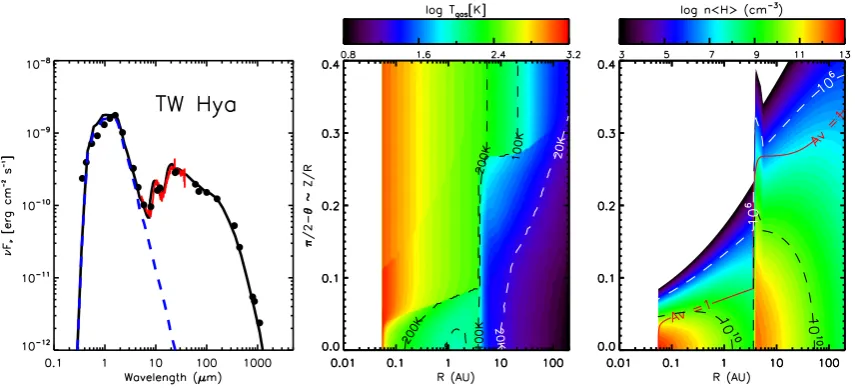
Figure 2.2Left panel: A 2-D model fit to the TW Hya SED using RADMC and the param-eters in Table 2.1. The stellar spectrum (peaking near 1 µm) is generated from a Kurucz model with Teff = 4000 K. The photometric points are taken from Rucinski & Krautter (1983), 2MASS, Low et al. (2005), and Weintraub et al. (1989), while the 5–35 µmSpitzer IRS spectrum is that displayed in Figure 2.1. Middle panel: Fiducial gas temperature pro-file. Right panel: Fiducial gas density profile, with the Av=1 height depicted by the solid

line.

temperature reaches 1400 K. The cavity radius is fixed asrcav = 4 AU, in accord with previous near-IR interferometry (Eisner et al., 2006; Hughes et al., 2007; Akeson et al., 2011). We adopt the power-law density profile of Andrews et al. (2012) for the outer disk, which is based on 870 µm continuum interferometric imaging. A summary of the dust structure model parameters can be seen in Table 1.

Following Pollack et al. (1994) and D’Alessio et al. (2001), we use a dust mixture of astronomical silicates, organics, and water ice. For the optically thin inner disk, pure glassy silicate is used to match the strong silicate bands at 10 and 18 µm. The dust size distribution is taken to be n(a)∝a−s _{with s = 3.5 between a}

min = 0.9 and

amax = 2.0 µm (Calvet et al., 2002). In the cavity wall, we use a dust size range between 0.005 and 1 µm; outside the cavity wall, 95% (by mass) of the dust has a size distribution extending from 0.005 µm to 1 mm, with the remaining 5% contained in grains from 0.005 – 1 µm. Total dust masses in the optically thin and thick parts of the disk are 2.77×10−9 _{and 4.4×10}−4 _M

Table 2.1. Disk parameters for the dust model

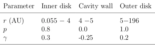
Parameter Inner disk Cavity wall Outer disk

r (AU) 0.055 − 4 4 −5 5−196

p 0.8 0.0 1.0

γ 0.3 -0.25 0.2

Note. — Here γ is the index that describes the vertical scale height zd: zd = z0(r/r0)1+γ where z0 = 0.7 at r0 = 10 AU; p is the index of the surface density distribution: Σd= Σ0(r/r0)−p.

temperature and density profiles, discussed further below, are presented in Figure 2.2.

2.4.2

The gas density and temperature

The gas/dust ratio in disks evolves due to grain growth and transport processes (Birnstiel et al., 2009), and likely has significant radial and vertical structure. For simplicity, the gas density is here assumed to follow that of the dust, with a constant gas/dust mass ratio throughout the disk. For TW Hya, the estimated global gas/dust ratio varies from 2.6 to 100 (Thi et al., 2010; Gorti et al., 2011). The recent detection of the HD J = 1-0 line from TW Hya has offered an independent and robust estimation of the gas mass (Bergin et al., 2013), which indicates a globally averaged gas/dust ratio close to 100, a value we adopt here. Significant dust vertical settling will produce an enhanced gas-to-dust ratio in the upper layers of the disk. Such settling should have little impact on the longest wavelength water transitions studied here, or on the strongest, optically thick lines traced by the Spitzer IRS. By creating a larger column of gas above theτdust = 1 surface, the absolute fractional abundance of water derived

to the dust distribution.

Above a certain altitude in the disk, where the environment becomes exposed to the ambient radiation field, the gas can also be thermally decoupled from the dust. The gas will adopt a temperature profile that is a balance among heating pro-cesses, such as mechanical heating via accretion or that driven by photodissociation or the photoelectric electric effect, and cooling rates driven by atomic, molecular, and dust grain emission (Glassgold et al., 2004; Kamp & Dullemond, 2004). General gas temperature profiles can be estimated using detailed thermo-chemical models (e.g. Woitke et al., 2009; Najita et al., 2011). However, such profiles can be highly depen-dent on input assumptions, and interdependencies between model parameters and observables can be obscure. Here, we simplify the process by deriving the vertical gas temperature structure in the inner disks using the rotational ladder from M-band CO P-branch v = 1−0 emission lines. Due to its (photo)chemical robustness, the abundance of CO is predicted to be fairly constant atnCO/nH2 ≈1.2×10

−4 _{in regions} warmer than 20 K (Aikawa et al., 1996). A high CO abundance is expected to persist even for a depleted inner disk, such as that of TW Hya. Indeed, in the chemical model of Najita et al. (2011), the abundance of CO rises to ∼10−4 _{once the vertical} column density of H2 reaches 1021 cm−2 for radii beyond 0.25 AU (physical densities are >109 _cm−3_).

Since the heating of the inner disk gas is driven by X-ray and FUV photons from the central star and stellar accretion flow (Kamp & Dullemond, 2004; Gorti et al., 2011), we assume that gas and dust temperature become decoupled in regions where the radial optical depth for visible photons is less than unity. That is,

Tgas=







Td, Av >1

Td+δT, Av 61

, (2.1)

where Td is dust temperature in the disk at (r,θ) in spherical coordinates, Av is the

4.66 4.68 4.70 4.72 4.74 4.76 4.78 0

5 10 15 20

4.66 4.68 4.70 4.72 4.74 4.76 4.78

Wavelength (µm) 0

5 10 15 20

Flux (10

-18

W.m

-2 )

δT = 120K

δT = 135K δT = 150K

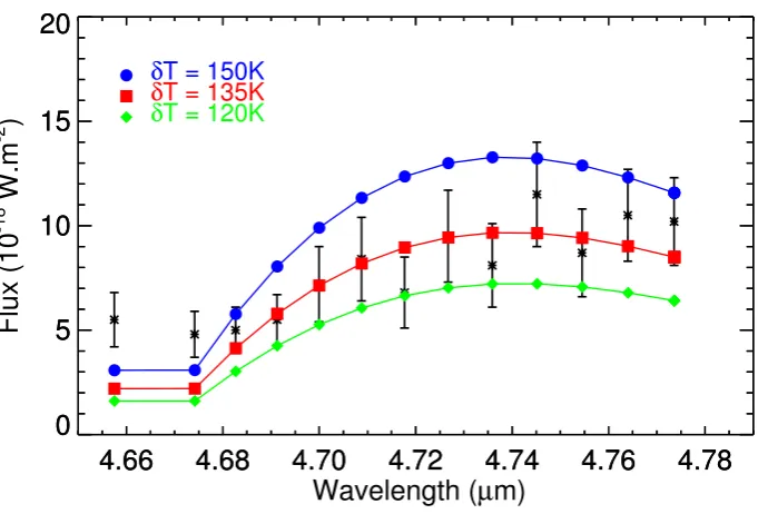
Figure 2.3 Model CO rovibrational fluxes from decoupled gas/dust temperature models compared with the observational data (depicted as crosses with error bars, from Salyk et al. 2007). The models show three different values of δT, the temperature difference between gas and dust, with values of 120 (diamonds), 135 (squares), and 150 K (circles).

The v=1-0 P(1-12) CO line fluxes at 4.7 µm are taken from Salyk et al. (2007), while the model spectra are generated by the raytracing code RADLite (Pontoppidan et al., 2009). The lines are ∼7.5 km/s wide (FWHM) (Pontoppidan et al., 2008), consistent with the nearly face-on orientation of TW Hya. The inner edge of the CO emission in the inner disk is set at rin = 0.11 AU, based on SA imaging of the 4.7 µm

line emission (Pontoppidan et al., 2008). The outer edge of the CO-emitting zone is not well constrained, and is set to 4 AU, the dust transition radius. The model is relatively insensitive to the size of the outer edge, since the majority of the emission is produced at radii 4 AU.

of NH = 1022cm−2. RADLite simulations predict a line width (prior to instrument profile convolution) of FWHM∼6.8-9.6 km/s forvturb ∼0.05vKepler. This is somewhat larger than observed 7.5 km/s linewidths, but this difference may be accounted for by the difference in disk inclination relative to that (i= 4◦) derived by Pontoppidan et al. (2008).

The best fit δT of 135 K applies only to the inner disk radii probed by CO, but similar physics will decouple the gas and dust temperatures near the disk surface at larger radial distances. To model this decoupling, we adoptTg =Td+δT×e−r/50 AUfor

the gas temperature at large scale heights, a parameterization that matches broadly the models of Thi et al. (2010) for TW Hya. Again, the gas density structure follows that of the dust.

We stress that such gas/dust thermal decoupling should have only a modest im-pact on a principle molecular mapping result presented here, namely the significant drop in the water vapor column density beyond the snow line. For the highest excita-tion lines measured byHerschel (and Spitzer) that trace the photon-dominated, and thus heated, layers in the inner disk and cavity wall, gas densities are at least ∼109 H2/cm3. Under such conditions the simulations of Meijerink et al. (2009) show that the emergent fluxes of the water lines detected here are within factors of two-three of their LTE values. Thus, the water vapor column densities should be reasonably well determined by LTE calculations whose temperature distributions are constrained by the CO M-band observations.

The outer disk is too cold to emit in such high excitation water lines, and as discussed further in Section 4.4, the physical density in theAv∼1 layer at radii beyond

5-10 AU is only ∼107 _H

to deplete in a similar manner, with the bulk of the vapor emission arising from an intermediate layer at densities where LTE calculations offer column density estimates good to within an order-of-magnitude (Hogerheijde et al., 2011).

2.5

Retrieving the radial water vapor profile

2.5.1

The water line model

Given the gas temperature and density structure for TW Hya, we can now constrain the water vapor content of the TW Hya disk surface as a function of radius. Our goal is not to provide an exacting description of the volatile abundances versus radius and height, but to determine what radial distribution of water vapor is most consistent with the available data.To this end, we construct a step function in water vapor abundance, with one value,Xinner, in the inner gas-depleted disk within 4 AU, another,

Xring, in a ring starting at 4 AU and extending to the snow line atRsnow, and an outer disk abundanceXouter. That is,

XH2O = 

   

   

Xinner, R <4 AU

Xring, 4 AU6R6Rsnow

Xouter, R > Rsnow

(2.2)

As described below, our calculations assume LTE but do account for line and contin-uum opacity. The XH2O values derived thus reflect the water vapor column densities

to different depths into the disk. Inside of 4 AU and for the longest wavelength Her-schel lines sensitive to the outermost radii the dust opacity permits the full vertical extent of the disk to be sampled. For the IRS features and the shorter wavelength PACS lines that sample gas near the transition radius, significant dust opacity limits the fitted column densities, and hence the XH2O values, to the upper layers of the

disk. Freeze-out and dust/line opacity greatly limit access to the midplane beyond 4 AU.

possible to identify subset of lines that co-vary. Consequently, we can explore one model parameter at a time to derive a best-fit model, illustrated in Figure 2.4. As we shall see, the simplest LTE model, namely a constant water abundance throughout the disk, is inconsistent with the data in hand.In Section 4.2.2, we further discuss whether the data support a modification to this basic structure in which the drop in water abundance beyond the snow line instead occurs over some finite, measurable distance.

To render model spectra, we set the level populations to LTE. While the critical densities (ncrit = 1010 −1012 cm−3) of the high energy mid-IR water transitions suggest that a non-LTE treatment is needed, there is currently no robust and fully tested LTE framework for the modeling of infrared water lines. That is, a non-LTE calculation is also likely to be inaccurate, given the uncertainty of collisional rates and the complexity of the transition network. Further, previous work suggests that non-LTE effects may alter line fluxes by factors of only a few for the moderate excitation lines detected here (Meijerink et al., 2009; Banzatti et al., 2012), which will preserve the qualitative aspects of our treatment. In setting level populations to LTE, we make it easier to reproduce our results and to evaluate the validity of our retrievals using more detailed models in the future.

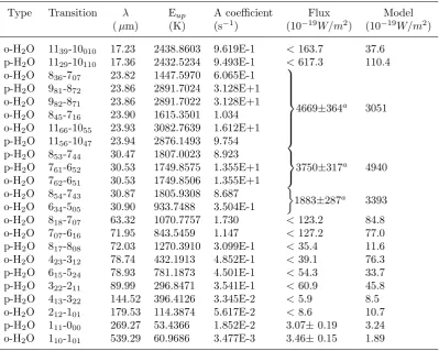
Table 2.2. Observed and calculated water line fluxes

Type Transition λ Eup A coefficient Flux Model

(µm) (K) (s−1_{) (10}−19_W/m2_{) (10}−19_W/m2₎

o-H2O 1139-10010 17.23 2438.8603 9.619E-1 <163.7 37.6 p-H2O 1129-10110 17.36 2432.5234 9.493E-1 <617.3 110.4 o-H2O 836-707 23.82 1447.5970 6.065E-1

              

4669±364a ₃₀₅₁ p-H2O 981-872 23.86 2891.7024 3.128E+1

o-H2O 982-871 23.86 2891.7022 3.128E+1 o-H2O 845-716 23.90 1615.3501 1.034 o-H2O 1166-1055 23.93 3082.7639 1.612E+1 p-H2O 1156-1047 23.94 2876.1493 9.754 p-H2O 853-744 30.47 1807.0023 8.923

 



3750±317a ₄₉₄₀ p-H2O 761-652 30.53 1749.8575 1.355E+1

o-H2O 762-651 30.53 1749.8506 1.355E+1 o-H2O 854-743 30.87 1805.9308 8.687

1883±287a 3393 o-H2O 634-505 30.90 933.7488 3.504E-1

o-H2O 818-707 63.32 1070.7757 1.730 <123.2 84.8 o-H2O 707-616 71.95 843.5459 1.147 <127.2 77.0 p-H2O 817-808 72.03 1270.3910 3.099E-1 <35.4 11.6 o-H2O 423-312 78.74 432.1913 4.852E-1 <39.1 76.3 p-H2O 615-524 78.93 781.1873 4.501E-1 <54.3 33.7 p-H2O 322-211 89.99 296.8471 3.541E-1 <60.9 45.8 p-H2O 413-322 144.52 396.4126 3.345E-2 <5.9 8.5 o-H2O 212-101 179.53 114.3874 5.617E-2 <8.6 10.7 p-H2O 111-000 269.27 53.4366 1.852E-2 3.07±0.19 3.24 o-H2O 110-101 539.29 60.9686 3.477E-3 3.46±0.15 1.89

2.5.2

Best-fitting model

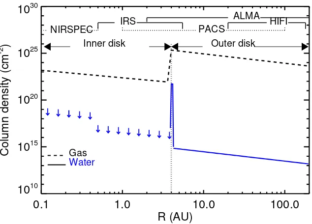
The best-fitting radial water column density profile in TW Hya is shown in Figure 2.4, whose spectral predictions are compared to the Spitzer LH data in Figure 2.5. We find that the inner optically thin region of TW Hya is dry, with upper limits on the vertically integrated fractional water abundance of Xinner < 10−6. The water detected by Spitzer originates in a thin ring near the disk surface, starting at 4 AU and ending at a snow line just beyond this at Rsnow ∼ 4.2 AU. At larger radii, the fractional water abundance drops abruptly by several orders of magnitude, to Xouter values near 3.5×10−11_.

The uniqueness of this solution is illustrated in Figure 2.6, which shows how variations in the water abundance in different regions of the disk affect different lines. This differential sensitivity is the foundation of our method for retrieving the radial column density, and thus abundance, profile, and are the subject of the following discussion.

2.5.2.1 The inner disk

The inner disk of TW Hya – radii within 4 AU – is partially cleared out, leading to integrated vertical column densities that are more than two orders of magnitudes lower than those typical for cTTs. The non-detection of water lines between 10 and 20µm, in the Spitzer SH range, may be a reflection of this, but even though the column density in the inner disk is dramatically reduced from the extrapolation of the outer disk to smaller radii, the scale height is sufficiently small that the physical densities at the Av∼1 surface exceed 109 H2/cm3. Thus, non-LTE effects are likely to be fairly unimportant, and we are able to produce meaningful upper limits on the fractional water abundance at r <4 AU.

sev-0.1 1.0 10.0 100.0 R (AU)

1010

1015

1020

1025

1030

Column density (cm

-2 )

Gas

Water

Inner disk Outer disk

NIRSPEC IRS PACS HIFI ALMA

14 16 18 20 22 24 a 1e-5 1e-6 1e-7 14 16 18 20 22 24 b 2.5e-3 2.5e-4 2.5e-5 14 16 18 20 22 24 c 3.5e-10 3.5e-11 3.5e-12

2 4 6 8 r(AU) 14 16 18 20 22 24 d

a1 a2 a3 a4 a5

0 0.1 0.3 0.5 0.7 0 a6

p-H2O

111-000

269µm

b1 b2 b3 b4 b5

0 0.1 0.3 0.5 0.7 0 b6

c1 c2 c3 c4 c5

0 0.1 0.3 0.5 0.7 0 c6

λ(µm)

d1

17.2017.30

λ(µm)

d2

23.7 24.0

λ(µm)

d3

30.5 30.8

λ(µm)

d4

63.3 63.4 λ(µm)

d5 179.4179.8 v (km/s) 0 0.1 0.3 0.5 0.7 0 d6

0 1 2 3 4 5 6

Water Column Density Log(cm

-2 )

Normalized Flux

IRS SH IRS LH IRS LH PACS PACS HIFI

eral water lines in the PACS range, especially the high excitation 63.3µm lines, while the Spitzer SH lines allow somewhat larger abundances. That is, the Spitzer SH spectrum tends to be consistent with a model in which the lack of lines below 20µm is explained by the overall low gas mass in the inner disk, and not necessarily a drier disk. It is the addition of the non-detection of PACS lines that require the fractional water abundance to be suppressed in the inner disk.

2.5.2.2 The transition region and the snow line

Next, we consider the origin of the water lines seen at 20-35µm. Figure 2.6 shows that the Spitzer LH lines detected are uniquely sensitive to variations in the water vapor content around the transition region. It is clear that a high water vapor col-umn density is required to fit the Spitzer spectra, with an emitting area close to

π×1 AU2. Our fiducial dust/gas model yields Xring ∼ 2.5×10−4 above the τdust=1 surface (line opacity is also significant). As discussed in §5.2, the required column density/abundance can be traded off against excitation temperature to some extent, with higher excitation temperatures corresponding to slightly smaller radii.

In the context of our transitional disk model, the most likely location for warm water vapor lies at the transition radius, or 4 AU, a prediction that can be tested by measurements of the water (or perhaps OH) emission line profiles using high resolution thermal-infrared spectroscopy. Interestingly, the cavity “wall” structure needed to reproduce the 10-30 µm SED (with a z/r value of 0.3) has a surface area close to that derived from the water emission for an inclination of seven degrees, further reinforcing the likely radial location of the high water vapor abundance.

Further, the PACS and HIFI lines are sensitive to the location of the snow line (the outer edge of the water-rich ring). Consequently, we varied the location of the snow lines between 4.2-6 AU. In Figure 2.6, it is seen that placing the snow line farther out in the disk over-predicts primarily the PACS lines. Hence, the detection of water lines by Spitzer in combination with the non-detection of water lines in PACS waveband provides strong constraints on the location of the surface snow line.

Because the water condensation temperature is a function of pressure and because of the strong vertical gradients in the disk, the local water vapor abundance need not precisely be a step function in radius. In particular, can the water lines between 40-150µm be used to constrain how rapidly the water abundance, as inferred from the column density structure, drops beyond the snow line with radius?

Specifically, we modify the abundance step function with an exponential drop-off beyond the snow line:

XH2O(R > Rsnow) = (Xring−Xouter)e

Rsnow−R R_eff

+Xouter, (2.3)

where Reff is the scale length of the abundance change. We consider Reff = 0.1, 0.5, and 1 AU, and find that models with Reff & 0.5 AU produce more flux than is observed by the Herschel PACS instrument (Figure 2.7). This supports our original assumption of a step function, and we conclude that the surface snow line in TW Hya is radially narrow; that is, it occurs over a region that is a small fraction of its distance to the star.

2.5.2.3 The outer disk

An extremely low vertically averaged abundance beyond the snow line,Xouter=3.5×10−11, is required by LTE fits to the HIFI ground state water lines at 267 and 537 µm. In-deed, the strongest constraint on the outer disk water vapor abundance is provided by the ground-state lines, although significant limits are also provided by slightly higher-lying transitions in the PACS range, in particular the 179.5µm transition. The low water vapor content of the outer disk is consistent with the analysis of Hogerheijde et al. (2011) and the HIFI non-detection of water lines in another transitional disk, DM Tau (Bergin et al., 2010). Specifically, our Xouter is comparable to the global disk-averaged value derived by Hogerheijde et al. (2011) – 7.3×1021 _{g of water in a} 1.9×10−2 _M

disk, or XH2O=2.2×10

Figure 2.7Constraints on the sharpness of the snow-line in TW Hya. The left panel shows model water vapor abundance decreases from XH2O∼2.5×10

−4 _{to 3.5×10}−11 _{with three} different radial scale lengths: 0.1 AU (dot line), 0.5 AU (solid line) and 1 AU (dash line). The right panel shows the modeled LTE line fluxes over-plotted onHerschel PACS spectra. The line styles are the same as in the left panel.

2.6

Discussion

From an analysis of the water emission lines from the TW Hya disk over the 10− 567 µm interval, both warm (∼220 K) and cold water vapor are found to be present. The warm water emission most likely originates in a narrow ring region between 4– 4.2 AU where abundant water vapor carries much of the cosmically available oxygen, XH2O ∼10

2.6.1

The origin of the surface water vapor

How does this study inform the origin of the observed water vapor, and of water in protoplanetary disks in general? There are two potential sources of water: one is in situ gas-phase formation, while the other is grain surface formation in a cold reservoir, which could be the disk itself or the primordial protostellar cloud. In the second case, a mechanism is needed to transport the ice inwards and upwards to a location where it can either thermally evaporate or be photodesorbed and observed in the form of vapor (see, for example, Supulver & Lin, 2000).

In the warm inner disk (r<1AU, z/r<0.2), H2O can be formed in the gas phase (Glassgold et al., 2009; Bethell & Bergin, 2009), even in the presence of substantial photolyzing radiation. The key is a sufficient supply of H2, which drives the forma-tion of water via successive hydrogenaforma-tion of atomic oxygen in reacforma-tions with sig-nificant activation barriers. More precisely, we find that using the photodissociation rate calculated only at Lyα (which dominates the 3×10−3L FUV continuum flux), and water reaction rates from Baulch, D. L. (1972) – kOH=3.0×10−14T e−4480/Tcm3 molecule−1s−1and kH2O=3.6×10

−11_{T e}−2590/T_cm3_molecule−1_s−1_{– this simplified} chem-ical model predicts water abundances near 10−4_whenT

g &200 K,ng>109cm−3. These

conditions are satisfied in the inner disk and the cavity wall, but not necessarily in the photon-dominated upper layers of the outer disk.

Thus, production of water via gas-phase reactions can potentially explain the high abundance of ∼220 K water vapor observed inside the TW Hya snow line, even if the initial conditions are atomic, and only until the elemental abundance of oxygen is depleted (∼5×10−4 relative to H, Frisch & Slavin, 2003). Indeed, modern thermo-chemical models (Woitke et al., 2009; Najita et al., 2011; Walsh et al., 2012) predict both that much of the oxygen is locked up in water vapor in the warm inner disk and at large scale heights where the gas is heated by UV and X-ray photons.

radius, the water abundance drops by two orders of magnitude, in conflict with this simple model. However, the models by Woitke et al. and Walsh et al. do not include the depleted inner region of TW Hya, making direct comparisons difficult for the innermost disk.

The warm gas-phase chemistry will not operate in the outer disk. Here, the primordial surface ice chemistry will dominate (Tielens & Hagen, 1982), resulting in a huge reservoir of icy dust and larger bodies from which water molecules must be thermally evaporated or desorbed by high-energy particles and photons. As discussed in Bergin et al. (2010) and Hogerheijde et al. (2011), models of photodesorption from icy grains find that a depletion of icy grains from the outer disk surface, presumably by setting to the midplane, is needed to reproduce the low observed outer disk water vapor abundances. A zeroth-order expectation is that the water vapor abundance across the snow-line can be treated as a step function (Ciesla & Cuzzi, 2006), with high inner disk water vapor abundances created by a mixture of gas-phase reactions and evaporating icy bodies and a low outer disk abundance maintained by desorption. We find a very low (vertically averaged) outer disk water abundance of a few times 10−11 _{per hydrogen, consistent with previous Herschel-HIFI observations, but} in conflict with the static thermo-chemical models, which indicate surface abundances of 10−7₋₁₀−9 _{per H. We interpret this as further evidence for settling of icy grains} in the outer disk of TW Hya.

Figure 2.8 The χ2 _{surface for LTE slab model water fits for TW Hya as a function of}

N andT, with an effective radiusR=1.0 AU. The contour plot is based onSpitzer IRS LH spectra, with best-fit parameters ofT = 220 K and N=1018_cm−2_{. The shadowed} area depicts the parameter space that is excluded by the water upper flux limits from the Spitzer IRS SH spectrum. Empty squares depict the best LTE slab model fit results for cTTs with water detections in the Spitzer-IRS wavelength range (Salyk et al., 2011).

2.6.2

The water vapor abundance distribution in transitional

disks

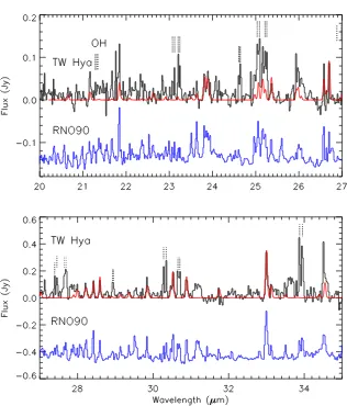
The Spitzer IRS spectrum reveals that the water vapor emission from TW Hya is different from that of typical, but less evolved, protoplanetary disks around solar-type stars. A comparison of the basic properties of the TW Hya water emission is shown in Figure 2.8, where an LTE slab model (disk-averaged) temperature and column density are compared to those of cTTs disks (Salyk et al., 2011). This is consistent with the detailed radial abundance structure derived for TW Hya.

snow line to reside in the optically thick outer disk. In contrast, many of the known transitional disks have transition radii of 10 AU or greater (Andrews et al., 2011), and the snow-line would be located well inside the optically thin region of the disk. They also typically lie two or three times more distant than TW Hya. Therefore, comparisons with additional transitional disks may need to wait for the availability of more sensitive instruments.

In contrast to the ∼1 AU snow line found by Meijerink et al. (2009) for cTTs disks, the TW Hya snow-line is located at a significantly larger radius, in spite of its lower luminosity as compared to DR Tau and AS 205 N. In the case of transitional disks, however, the exposure of the transition radius to nearly unobstructed stellar light and the ‘face on’ nature of the cavity wall at the transition radius should heat the disk more readily at large radii and push the snow-line outwards. One interesting consequence of this property is that if giant planets form and clear out a hole in the disk, creating a transitional disk, the subsequent migration of the snow line to larger radii could slow the growth of new planetary cores over a larger range of radii, out to the location of the new snow line.

At the same time, new planetesimal formation may be catalyzed near the new snow line due to enrichment of water by a combination the radial cold finger effect of Stevenson & Lunine (1988) and inwards radial migration of icy bodies (Ciesla & Cuzzi, 2006). The observed high abundance of water around 4 AU in TW Hya is supportive of a scenario in which new icy planetesimal formation, and perhaps even giant planet formation, is ongoing at this location.

Another interesting feature of the distribution of water vapor abundance in TW Hya is the relatively dry inner disk. The water vapor abundance in the innermost disk (<0.5 AU) is actually unconstrained by the Spitzer data due to beam dilution, but for r >0.5 AU the abundance upper limit is two orders of magnitude below that estimated in cTTs disks, and the lack of water in inner disk can be explained by two possible scenarios.

ring around 0.5 AU plus an outer optically thick disk starting at 4 AU can match the full suite of near-IR interferometric data and the general SED shape of TW Hya. Recent 8 - 18 µm speckle imaging, however, has suggested a more continuous dust distribution out to 4 AU and perhaps the presence of a companion (Arnold et al., 2012).

Furthermore, analysis of the ALMA CO J=2-1 and 3-2 Science Verification ob-servations of TW Hya has revealed gas signatures down to radii as close as 2 AU (Rosenfeld et al., 2012). Thus, the more likely scenario for the structure of the TW Hya disk is that outlined in Figure 2.4, namely an inner disk in which CO remains abundant, since the kinetic temperature is much higher than that needed for freeze-out (∼20 K).Water in the inner disk can still be subjected to some depletion, or in the case that a companion gates the accretion flow into the inner disk any water-ice rich grains that settle to the (outer disk) mid-plane may be blocked from further inward migration. If this is the case, there should be a large difference in the gas phase C/O ratios between the inner and outer parts of the disk. Thus, the quantity of gas along with its C/O content potentially probes that can distinguish whether a given transition disk has been sculpted by planet formation or other mechanisms (grain growth or photo-evaporation, for example; see Najita et al. 2011 for further discussion of how changes in the C/O ratio can impact disk chemistry).

A final aspect of these observations is the short scale length (<0.5 AU) over which the dramatic water vapor decrease occurs, a distance in conflict with scenarios that consider only freeze-out. Such a radial profile may be further evidence for a vertical cold finger effect, in which the surface snow-line location reflects that at the mid-plane, perhaps due to mixing (Meijerink et al., 2009).

2.6.3

Molecular mapping with multi-wavelength spectra

observed to date are in accord with the changing physical conditions that passive cTTs disks experience as they evolve. Much more detailed constraints and comparisons to models will become available over the coming years by exploiting the significant infrared database that exists for stars+disks of varying mass and evolutionary state (Pontoppidan et al., 2010b; Salyk et al., 2011) along with new observations at longer wavelengths.

Because protoplanetary disks are complicated structures, the multi-wavelength molecular mapping method should be used with some caution, however. The flux of each line will arise from a range of disk regions, with lines at various wavelengths characterizing different radii and/or vertical depths, and an overview of several of the key water vapor tracers for the best fitting TW Hya model is presented in Fig. 2.9. As demonstrated in this work, it can take considerable effort to build realistic models for an individual source, and efforts herein were aided by a large set of ancillary observations of this well-studied disk. Nevertheless, it is important to stress that relatively fewer uncertainties are introduced in this type of modeling than with the use of full thermal-chemical disk models, in which chemical abundances are sensitive to a wide array of model parameters, including FUV and X-ray fluxes, accretion rate, disk viscosities and transport rates, dust-versus-gas settling geometries, grain-surface reaction rates, and so on (e.g. Heinzeller et al., 2011). Further, studies of large disk samples will require fast, robust models. We therefore advocate for the direct measurement of chemical abundances with relatively few free parameters, such as is described in this work, to be used in conjunction with physical intuition derived from the more complex thermal-chemical models.

of lines with a significant range of excitation energies will provide the most stringent probes. This technique thus provides an ideal means to study chemical structure at the size scales relevant to planet formation.

With a properly chosen spectral suite, we have demonstrated that it is possible to probe molecular abundance distributions on AU scales, and it is worth emphasizing that this method is highly complementary to the capabilities of ALMA. At its longest baselines (16 km), the full ALMA will be able to resolve a nearby disk (140 pc) on AU scales at its shortest operational wavelength, ∼400 µm, in dust emission. However, due to the quantum-limited nature of heterodyne receivers and the available collecting area, it will be a severe challenge even for ALMA to robustly image the warm molecu-lar gas inside of 10 AU – the principle formation region of terrestrial and giant planets according to core accretion theory. Thus, for the foreseeable future, multi-wavelength methods (which can incorporate ALMA spectral data cubes) offer perhaps the best means of deriving the molecular abundance patterns in planet-forming environments. Table 2.3 presents the general selectivity of each wavelength window for disks around Sun-like stars.

Table 2.3. Volatile line tracers at different disk radii

Wavelength Radius Facility

µm AU

2-5 0.1 NIRSPEC, CRIRES

6-10 0.1- 1 SOFIA FORECAST

10-35 0.5- 5 Spitzer IRS

40 - 200 1-100 Herschel PACS 200- 30000 >50 HIFI, ALMA

Figure 2.9 The radial and vertical locations bounding water vapor emission from the TW Hya disk. The boxes mark the 15% and 85% cumulative radial line flux limits (vertical lines) and the heights where 15% and 85% of the line flux arises from each vertical column (horizontal lines). The gas density of the disk is shown in greyscale, and the location of the Av∼1 gas/dust decoupling transition (Tg =Td) is shown by

the dotted line. As a guide to the eye, the nH2 = 10

2.7

Conclusions

This paper uses multi-wavelength spectra to probe the water vapor distribution in protoplanetary disks, and demonstrates the first application of this method to in-vestigate the water vapor abundance from 0.5-200 AU in the transitional disk TW Hya. Our modeling shows that there is a narrow region between 4-4.2 AU where water vapor is warm (∼220 K) and optically thick, resulting in a high abundance (XH2O∼10

−4_{). Outside the snowline, the water vapor column density in the disk} at-mosphere decreases dramatically over a scale length of less than 0.5 AU due to freeze out, resulting in a vertically integrated vapor abundance of XH2O∼10

Chapter 3

Comparison of the dust and gas

radial structure in the transition

disk [PZ99] J160421.7-213028

Ke Zhang

, Andrea Isella

, John M. Carpenter

, Geoffrey A. Blake

1. Division of Physics, Mathematics & Astronomy, MC 249-17, California Institute of Technology, Pasadena, CA 91125, USA; [email protected]

2. Division of Geological & Planetary Sciences, MC 150-21, California Institute of Technology, Pasadena, CA 91125, USA

Keywords: Stars: pre-main sequence; planetary systems: protoplanetary discs; submillimeter: stars

3.1

Abstract

3.2

Introduction

Planets form in the disks orbiting young stars, but the paths by which the primordial gas and dust accumulate into planetary bodies remain unclear. The capabilities of new optical, infrared, and (sub)-millimeter telescopes can place constraints on the planet formation process by mapping the gas and dust emission of planetary systems in the act of formation. Transition disks, defined by their significantly reduced infrared emission at wavelengths <8µm compared to the median disk emission (Strom et al., 1989; Wolk & Walter, 1996), are of particular interest. The relative lack of infrared emission implies the absence of warm dust in the innermost disk. This dust depletion might be a manifestation of the early stages of planet formation as a result of the dynamic interactions between the disk and forming giant planets (Lin & Papaloizou, 1979; Artymowicz & Lubow, 1994), but other mechanisms can suppress near-infrared dust signatures without the pr