Constructing informative Bayesian map priors: A multi-objective optimisation approach applied to indoor occupancy grid mapping

This is a repository copy of

Constructing informative Bayesian map priors: A

multi-objective optimisation approach applied to indoor occupancy grid mapping

.

White Rose Research Online URL for this paper:

http://eprints.whiterose.ac.uk/111297/

Version: Accepted Version

Article:

Georgiou, C., Anderson, S. orcid.org/0000-0002-7452-5681 and Todd, T. (2017)

Constructing informative Bayesian map priors: A multi-objective optimisation approach

applied to indoor occupancy grid mapping. The International Journal of Robotics

Research. ISSN 0278-3649

https://doi.org/10.1177/0278364916687027

Reuse

Unless indicated otherwise, fulltext items are protected by copyright with all rights reserved. The copyright exception in section 29 of the Copyright, Designs and Patents Act 1988 allows the making of a single copy solely for the purpose of non-commercial research or private study within the limits of fair dealing. The publisher or other rights-holder may allow further reproduction and re-use of this version - refer to the White Rose Research Online record for this item. Where records identify the publisher as the copyright holder, users can verify any specific terms of use on the publisher’s website.

Takedown

If you consider content in White Rose Research Online to be in breach of UK law, please notify us by

Constructing informative Bayesian map priors: a

multi-objective optimisation approach applied to

indoor occupancy grid mapping

Christina Georgiou

_{, Sean Anderson}

_{and Tony Dodd}

January 27, 2017

Abstract

The problem of Simultaneous Localisation And Mapping (SLAM) has been addressed in numerous ways with different approaches aiming to pro-duce faster, more robust solutions that yield consistent maps. This focus, however, has resulted in a number of solutions that perform poorly in chal-lenging real life scenarios. In order to achieve improved performance and map quality this paper proposes a novel method to construct informative Bayesian mapping priors through a multi-objective optimisation of prior map design variables defined using a source of prior information. This concept is explored for 2D occupancy grid SLAM, constructing such pri-ors by extracting structural information from architectural drawings and identifying optimised prior values to assign to detected walls and empty space. Using the proposed method a contextual optimised prior can be constructed. This prior is found to yield better quantitative and qualita-tive performance than the commonly used non-informaqualita-tive prior, yielding an increase of over 20% in theF2 metric. This is achieved without adding

to the computational complexity of the SLAM algorithm, making it a good fit for time critical real life applications such as search and rescue missions.

SLAM, Bayesian estimation, informative priors

1

Introduction

Bayesian methods dominate the estimation algorithms used in Simultaneous Lo-calisation and Mapping (SLAM) (Durrant-Whyte & Bailey 2006), yet there has been very little research to date into how to effectively construct the Bayesian

∗_{Department of Automatic Control and Systems Engineering, The University of Sheffield,} Sheffield, S1 3JD, United Kingdom

†_{PA Consulting}

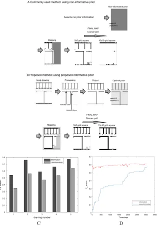
Figure 1: The structure of the SLAM problem: sensor data, prior information and motion model predictions are input to the SLAM algorithm that recursively maps the environment and localises the robot within it; architectural drawings and floor plans can be used to extract prior information. The commonly used Bayesian prior is constructed assuming there is no available information about the environment and so is uninformative. The proposed Bayesian prior is con-structed using available information that is processed and placed in an optimised prior format.

map prior using available information. This is the case even though the use of priors is a key distinguishing feature of Bayesian estimation. The lack of atten-tion given to the map prior can be contrasted to the enormous wealth of raw prior information that is readily available and untapped for most mapping and localisation scenarios, such as architectural drawings for buildings, city maps for the urban environment, geographical surveys for the wider outdoor environment and even pipe network maps for the underground environment. There exists an important and unsolved problem, therefore, in how to optimally synthesize raw prior information into a form that is suitable for robot navigation. This paper addresses this problem for 2D indoors occupancy grid SLAM by proposing a novel method to construct contextual priors that can improve the performance of robot navigation using architectural drawings and floor plans as a source of prior information (Figure 1).

The idea of using prior information to improve the performance of robotics systems has been suggested for a number of systems that operate in real-world, challenging environments. Priors are used in self-driving cars to improve locali-sation (Maddern, Pascoe & Newman 2015) and 3D semantic priors are used to interpret traffic lights (Barnes, Maddern & Posner 2015). Prior knowledge can be incorporated in feature-based SLAM by using known landmarks (Burschka, Geiman & Hager 2003). Implementations such as (Williams & Reid 2010) use only a few known landmarks as points of reference to correct predictions and (Parsley & Julier 2011) constrain the possible location of landmarks in Graph-SLAM using prior information. As a result, the observed position error is re-duced whilst maintaining the same or improved consistency compared to the no-prior solution (de la Puente & Rodriguez-Losada 2014). Finally, skeletal SLAM (Milstein 2005) uses prior information about the shape of a building to construct more accurate occupancy grid maps.

In all of the above cases the use of prior information was found to be bene-ficial and yield improved performance in robot navigation. However, all of the methods reviewed above define the prior in an ad-hoc way, without using any particular method to choose prior probabilities from raw prior data. There is a gap, therefore, in constructing Bayesian map priors from available data using a formal, methodological approach, that can be optimised and repeated across different mapping scenarios. The main contribution of this paper is a novel method to construct contextual Bayesian map priors that improve map quality. Georgiou2015 proposed the use of architectural drawings and floor plans as a source of prior information, presenting a novel method to extract wall and empty space locations from such drawings. The paper presented a method to extract information that can be used to construct the prior map, but did not explore how to construct and use such a prior map using detected walls and empty space. Building on (Georgiou, Anderson & Dodd 2015), we aim to determine optimised values to assign to detected walls and empty space. The maps produced using these optimised values are tested in both simulation and experiment. The optimised Bayesian prior map is benchmarked here against the use of a non-informative prior, and the results demonstrate that the use of the optimised prior is hugely beneficial in the initial period of mapping and localisation, and retains an improvement in the final map. These results suggest that optimised Bayesian priors have great potential, especially in time-critical missions such as search and rescue.

an optimal trade-off surface - a Pareto-optimal front. From the Pareto-front, the user can choose an appropriate trade-off between precision and recall to define the Bayesian prior map.

In summary, the following four steps are proposed as a solution to construct-ing informative Bayesian priors: 1. identify a source of prior information and a method to extract useful information from it; 2. determine prior map design variables that affect final map quality; 3. define quantitative measures of map quality - precision and recall; and 4. perform a multi-objective optimisation to identify prior probabilities that yield high performance metrics.

This paper is organised as follows. Section 2 gives an overview of the role of priors in SLAM and shows how using an optimised Bayesian prior can yield performance improvements. Section 3 presents the proposed strategy to con-struct informative priors and explains each aspect for the case study explored in this paper, indoors occupancy grid mapping. Section 3.1 presents the algo-rithm used to extract the location of walls from an architectural drawing or floor plan. Section 3.2 details a novel quantitative measure of map quality and Section 3.3 presents a multi-objective optimisation using a genetic algorithm to identify Pareto optimal design parameters. Section 4 presents the image test set used to demonstrate results in this paper and details the simulation used to obtain mapping results. Section 5 compares the maps produced in simulation using various shortlisted priors to determine which are optimal and presents the benefits of the proposed prior construction method. Finally, Section 6 validates the benefits of using an informative prior experimentally, both in a simulated robot course and in a large scale experiment.

2

Bayesian priors in SLAM

SLAM aims to have a robot explore and map an environment whilst simultane-ously localising itself within it. The robot uses sensors to perceive the environ-ment, a motion model or odometer to predict robot motion and it can also use a prior to incorporate information about the environment (Durrant-Whyte & Bailey 2006). Each of the elements of the chosen implementation for this paper are presented in this section.

First the probabilistic formulation of SLAM is given, highlighting the role of the prior map. The implementation of choice, occupancy grid FastSLAM (Montemerlo, Thrun, Koller & Wegbreit 2003), is then presented, showing the separation of the localisation and mapping tasks using Rao-Blackwellization, and the incorporation of prior information through the occupancy grid mapping algorithm is highlighted. This separation allows a study of mapping without the need to focus on performing localisation.

2.1

Probabilistic formulation

pose. Formally, it aims to compute the joint posterior of the robot’s pose xk

and the mapm(Durrant-Whyte & Bailey 2006)

p(xk,m|Z0:k,U0:k,x0)∝A×p(m) (1)

for all times k. xk is the state vector describing the robot’s pose,m is the

map of the environment (or a selection of landmarks for feature-based SLAM),

p(m) is the prior map, Z0:k are the sensor observations, U0:k the history of

control inputs andx0is the robot pose at time k= 0. Ais given by

A=p(zk,xk|m)

p(xk,m)

p(xk,m|Z0:k−1,U0:k,x0)

p(zk|Z0:k₋1,U0:k)

(2)

since the joint posterior in (1) can be written

p(xk,m|Z0:k,U0:k,x0) =

p(zk|xk,m)

p(xk,m|Z0:k₋1,U0:k,x0)

p(zk|Z0:k−1,U0:k)

=p(zk,xk|m)

p(xk,m)

p(m)p(xk,m|Z0:k−1,U0:k,x0)

p(zk|Z0:k₋1,U0:k)

∝A×p(m)

(3)

indicating that the joint posterior is proportional to the prior probabilityp(m).

Therefore a choice of an optimised prior p(m) can lead to a more accurate

estimate of the joint posterior.

The aim is to estimate the robot pose for all times k and the map of the

environment given sensor readings, control inputs and a starting pose. SLAM is solved recursively, producing map and pose estimates at each time step.

In the probabilistic formulation of SLAM the tasks of localisation and map-ping cannot be viewed separately. FastSLAM uses Rao-Blackwellization to sep-arate localisation and mapping as discussed in the following section. Therefore FastSLAM allows the study of the effects of a prior map without the need to address the localisation aspect of SLAM.

2.2

Occupancy grid FastSLAM formulation

FastSLAM uses Rao-Blackwellization to decompose the SLAM problem into a robot localisation problem and a collection of landmark/map estimation prob-lems that are conditioned on the robot trajectory estimate (Montemerlo et al. 2003), (Durrant-Whyte & Bailey 2006).

p(X0:k,m|Z0:k,U0:k,x0)

=p(m|X0:k,Z0:k)p(X0:k|Z0:k,U0:k,x0)

(4)

In this case the aim is to compute the joint posterior of the map and the

complete robot trajectoryX0:k rather than the single posexk. That is because

landmarks conditioned on the trajectory are independent, allowing the factori-sation shown in Equation 4. A particle filter can then be used to sample from the motion model and produce the proposal distribution but now the estimates for the landmark locations (conditioned on the robot trajectory estimate) are performed separately.

Since the pose and map estimates can be performed separately using Rao-Blackwellization, the occupancy grid mapping algorithm can be used to

calcu-latep(m|X0:k,Z0:k). The starting posex0is considered to be deterministic for

the purposes of this paper, since for a known prior map we can measure pose

x0 at t = 0 with respect to the prior map, similarly to the minimum

covari-ance case in (Dissanayake, Newman, Clark, Durrant-Whyte & Csorba 2001). Therefore prior information about the environment can only be incorporated

intop(m|X0:k,Z0:k) through the Bayesian priorp(m).

The occupancy grid mapping algorithm (Elfes 1989) is used in this paper to update the probabilities of occupancy of each grid cell in the environment.

This representation is chosen since the prior mapp(m) is the map used at time

k= 0, which is then recursively updated as occupancy measurements are taken

for map cells as the robot explores the environment.

The occupancy grid mapping algorithm (Elfes 1989) splits the environment to be mapped into a grid of cells and a prior probability is assigned to each cell. The log odd occupancy of each grid cell can be updated using

l_{k,i=InverseSensorM odel(}m_i,x_k,z_{k) +}l_k−1,i−l0,i (5)

with

lk,i=log

p(mi|Z1:k,x1:k)

1−p(mi|Z1:k,x1:k)

(6)

A detailed derivation of Equation 5 is given in the Appendix.

The Bayesian priors for each cell,p(mi), are incorporated through l0,i, the

log odds prior for a given cell. When there is no available prior information a

non-informative Bayesian prior is assigned to all grid cells, p(mi) = 0.5, i =

1, ..., N. Most researchers use such a prior in order to produce solutions that do not depend on having prior knowledge of the environment (Durrant-Whyte & Bailey 2006). Others claim that access to information such as detailed ar-chitectural drawings may be difficult (Kumar, Rus & Singh 2004). Information such as floor plans for buildings like hospitals and offices is generally available, however, and can be used to extract useful information and construct SLAM priors.

Incorporating prior information does not add to the computational cost of running SLAM and only incurs a one-off cost of extracting prior information and constructing a prior. Since the posterior is proportional to the prior map (Equation 3) and given the recursive nature of SLAM, constructing an

infor-mative prior mapp(m) can help produce a more accurate map even if a quick

only be scanned once or twice, making the effect of the prior more significant. This is especially useful for time critical applications where the environment needs to be explored quickly, such as USAR missions.

3

Proposed approach

The proposed strategy to convert prior information to an informative Bayesian prior is presented in this section. This consists of the following steps

1. . A method to process a source of prior information such as an aerial image or architectural drawing to extract relevant prior information

2. . A set of prior map design variables that affect final map quality

3. . A set of metrics to assess the quality of the final map which can be used to select optimised design variables

4. . A multi-objective optimisation to identify design variables that yield high map quality metrics

The rest of this paper discusses each of those aspects for the case study of indoors occupancy grid mapping using architectural drawings and floor plans as a source of prior information.

3.1

Extracting structural information from an

architec-tural drawing

In order to construct optimised priors an appropriate source of information needs to be identified. This can be an image such as an architectural drawing or floor plan for indoors SLAM or an aerial photograph or road network map for outdoors SLAM. These drawings or images then need to be processed to extract the location of occupied and unoccupied environment sections. For indoors environments, walls and empty space need to be identified. Similarly, if the source of prior information is a road map, roads and non-traversable areas can be detected. This paper focuses on the use of architectural drawings as a source of information and so this section presents a method to extract structural information from them to construct a prior map.

Structural information such as the location of building walls is required in or-der to construct an indoors prior map. Architectural drawings and floor plans, two-dimensional, top-down drawings of buildings containing structural infor-mation, suggested furniture and annotated text can be used to extract such information. These need to be processed to extract structural information in order to construct a meaningful prior map of the environment. Once the loca-tions of structural elements such as walls have been determined, they can be

used to assign appropriate prior valuesp(mi) to all grid cells.

(a) (b)

Figure 2: (a) Symbols for different types of doors (doors drawn using floor-planner.com) (b) The majority of door types can be approximated as isosceles triangles (drawn in grey).

information that can be used to construct robot priors. The main problem with processing drawings to extract this information is the lack of consistent representations between different drawings (Figure 2(a)). Depending on the architect and drawing method used, doors, walls and other elements can be represented in a different manner. Therefore, in order to yield reliable results for any drawing, the algorithm used to extract structural information needs to be independent of the drawing style.

The information the algorithm aims to extract is the location of walls which can be easily put in an occupancy grid format by assigning detected walls a low prior probability of being empty and detected space a high prior probability. Walls are represented as dark lines in the majority of drawings but have no other distinct geometric features. Given this variation between drawings, using methods such as line thickness to determine wall locations is unreliable. Instead of searching for walls directly, a feature with distinct geometric features and a clear relation to walls is detected. Doors are chosen for their distinctive shape and because they connect wall segments. Therefore if the location of doors in the image is found walls can also be detected.

There is no universally used symbol for all doors (Baden-Powell, Hetreed & Ross 2011) and depending on the type of door (single, double, sliding, foldable, etc., Figure 2(a)) and the way the drawing was produced (different drawing software, hand-drawn) different representations can be used. However, all door symbols share a geometric characteristic: they can be approximated as isosceles triangles defined by three vertices and (usually) two edges/connected sides as shown in Figure 2(b). The proposed algorithm therefore searches for triangles in the image (as defined by their vertices) that fulfill the isosceles triangle criteria.

This algorithm has a computational cost of O(n3) where n is the number of

Harris Corners detected in the image and it is dominated by the cost of finding

the possible combinations nCr = n!

r(n₋r)! of r = 3 out of n detected Harris

corners.

Once wall locations have been extracted from an architectural drawing, prior

occupancy valuesp(mi) need to be assigned to each grid cell mi accordingly.

Three parameters have to be chosen:

• Prior probability assigned to detected walls

Algorithm 1Drawing Processing Algorithm

FindHarrisCorners(Drawing)

PossDoors ←AllUniqueThreeCornerCombinations

DoorsShortlist←[ ] for_{i=1:size(PossDoors)}do

if _{SideCheck(PossDoors(i)) & AngleCheck(PossDoors(i))} then if _{ConnectivityCheck(PossDoors(i))}then

DoorsShortlist←[DoorsShortlist, PossDoors(i)] end if

end if end for

DetectOuterWalls(Drawing)

DetectedDoors←RemoveFalsePositiveDoors(DoorsShortlist)

FindWalls(Drawing, DetectedDoors)

• Occupancy grid cell size (grid resolution)

Each grid cellmiis assigned a Bayesian prior probabilityp(mi) (Section 2.2).

The following notation will be used throughout the rest of the paper. A high probability assigned to a grid cell will mean the cell has a high probability of being empty. Conversely, a low probability will signify a low probability that a cell is empty. If wall locations are known, cells that are located where walls

were detected can be assigned lower prior probabilities,p(mwall

i )<0.5, and cells

located where empty space was detected can be assigned higher prior

probabil-ities,p(mspace_i )>0.5. For brevity these two probabilities will be writtenpwall

andpspace, wherepwall is the prior probability assigned to grid cells that

corre-spond to locations of detected walls in the architectural drawing andpspacethe

prior probability assigned to cells corresponding to detected empty space in the

drawing. This notation can be used since all grid cellsmi that correspond to

occupied locations will be assigned a prior probability ofpwall and those that

correspond to empty space a prior probabilitypspace.

The alignment of grid cells and detected walls depends on the occupancy grid cell size. In all the results presented an appropriate grid cell size was chosen for all drawings used. The effects of using priors when coarser grids are used are discussed in the results section.

3.2

Map quality assessment

Using the method described in Section 3.1 walls and empty space can be detected in architectural drawings. Prior values of occupancy then need to be assigned

to each grid square. In order to determine which (pwall, pspace) pair yields

optimal performance the problem of assessing map quality is presented as a binary classification problem and a precision-recall analysis is performed.

& Stachniss 2014), there is no consistent notion of consistency and determining whether or not a SLAM map is consistent is still an open problem. Global consistency is often used to mean that the map produced agrees with the ground truth whereas local consistency refers to correctly aligning sensor scans locally. A measure for global consistency is proposed in (Mazuran et al. 2014) which uses the mismatch in the sensor data but this framework is tailored to SLAM using 2D laser sensors and can struggle in dynamic environments. (Collins, Collins & Ryan 2007) compute a correlation between the produced map and ground truth but this tends to be computationally expensive.

In this paper we propose a metric that is easy to evaluate and that gives an indication of how successful the system was in detecting occupied and empty space in the environment. The use of the percentage of free and occupied cells identified correctly is proposed as a performance metric in (Grewe, Komar, Hohm, Lueke & Winner 2012). The novelty of our proposed approach is the formulation of the assessment of the quality of an occupancy grid map as a clas-sification problem where the aim is to correctly classify pixels as corresponding to occupied or unoccupied space. Therefore a precision-recall analysis can be used to evaluate the quality of the produced maps. Occupied locations in the environment can then be defined as true positives and empty space as true negatives. Any other objects detected can then be defined as false positives.

The chosen metrics are therefore detailed as follows (Davis & Goadrich 2006):

• P recision(pre) = T rueP ositives

DetectedOccupiedSpace

• Recall(rec) = T rueP ositives

ActualOccupiedSpace

with precision representing the percentage of correctly detected walls and recall representing the number of walls correctly detected out of all walls in the drawing.

Following these assessment criteria, each point in the robot map is tested against the true environment to determine whether it has been classified cor-rectly. A simple way to perform this comparison in practice is to find the difference between the true environment image and the produced map to iden-tify false positives and false negatives and thus calculate the above metrics. This is a simple but effective and computationally inexpensive method to assess quantitative performance.

Constructed priors are tested in a simulation which assumes perfect knowl-edge of the robot’s pose so over or underestimating these values if the map and ground truth images are misaligned is not a problem. Therefore this method of comparing the map to ground truth to find the number of true/false posi-tives/negatives is used to test the performance of maps produced using different priors.

to a lower precision. A coarse grid would assign all cell pixels as occupied for a cell made up of mostly occupied space. For a large cell size this would result in incorrectly assigning many map pixels to occupied space, thus reducing precision. This would result in an area of misclassified points that are not strictly a classification error, just a limitation of an unsuitable grid resolution. In order to avoid penalising a system with an unsuitably coarse grid resolution, maps that perform well quantitatively are also tested qualitatively to ensure overall good performance.

While testing different prior maps for different drawings it was observed that the objectives of maximising precision and maximising recall are conflict-ing. Therefore selecting optimal prior values to maximise both objectives is not trivial and a multi-objective optimisation is proposed to determine optimised prior values.

3.3

Multi-objective optimisation to optimise prior

param-eters

In order to test how the values for (pwall, pspace) that yield maximum

preci-sion and recall compare in a qualitative sense, maps can be constructed using

the prior (pwall, pspace) values yielding maximum precision and recall. These

can then be tested to assess the qualitative performance of maps produced using these prior values. If requirements for each metric are conflicting a

multi-objective optimisation can be performed to determine pairsπ = (p_wall, p_space)

that yield both high precision and high recall. Having both precision and recall

>40% was empirically determined to be an acceptable threshold.

This multi-objective problem can be formulated as

min π

F(π) = [f_pre(π) f_rec(π)]

subject to C=



 

 

0.1≤π<1

fpre(π)<2.5

frec(π)<2.5

(7)

where π = (p_wall, p_space), f_pre(π) = 1

pre and frec(π) = 1

rec (so fpre(π),

frec(π)<2.5⇔pre, rec >40%).

In order to perform this multi-objective optimisation a Pareto-based method was chosen since the relative importance of the objectives is unclear (Giagkiozis, Purshouse & Fleming 2015) and a controlled elitist genetic algorithm (Deb 2001) (a variant of NSGA-II (Deb, Pratap, Agarwal & Meyarivan 2002)) was used.

In this minimisation problem a decision vector ˆπ with ˆπ ∈ C is Pareto

optimal if there is no otherπ∈Cfor whichf_i(π)≤f_i( ˆπ), ∀iand at least one

fi(π)< f_i( ˆπ) for i= 1, ..., K where K is the number of functions inF(π). In

this case the decision vector ˆπ is said to Pareto-dominate vectorπ. If only the

multi-objective optimisation solver used aims to find a subset of Pareto optimal solutions which is referred to as the Pareto front (Giagkiozis et al. 2015).

The concept of Pareto dominance is applied in order to use a genetic al-gorithm to solve this multi-objective problem. First the objective function is

evaluated for each individual in the population Π. Non-dominated

individu-als, Πnond are then found and removed from the population. This process is

repeated until all non-dominated individualsΠnond have been identified.

In order to obtain recall and precision variables and perform the multi-objective optimisation a simulation environment was devised as detailed in the next section.

4

Simulation setup

A simulation was used to produce maps using different (pwall, pspace) pairs.

A simulation allows the testing of a large number of possible prior values to

assign to (pwall,pspace). Thus the multi-objective optimisation can be performed

without the need to obtain mapping results for different buildings using a robot which would be very time consuming. The drawing test set, simulation used and assumptions made are discussed in this section.

4.1

Drawing test set selection

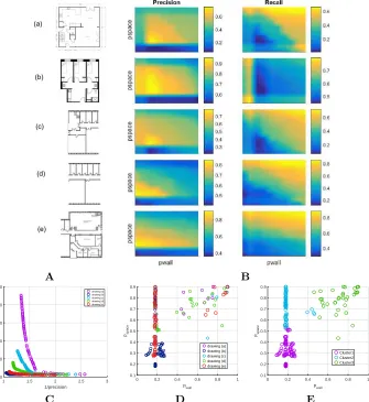
A number of different drawings were tested using the simulation environment described in this section. A version of each drawing containing only structural information was created by hand and used as the ground truth. Two floor plans, drawings (a) and (b) in Figure 4A, are presented, with drawing (a) containing labeling and drawing (b) containing suggested furniture. Drawings (c), (d) and (e) in Figure 4A, are sections of an architectural drawing of a University of Sheffield Engineering building. These sections were chosen because they are a representative sample of different outlines and commonly observed elements. Drawing (d) contains only doors and wall segments making it an easy drawing to process and drawings (c) and (e) are quite challenging to process, containing stairs, text, walls of varying width and, in the case of drawing (e), a door at an angle. These were chosen as a representative sample of common elements and configurations found in architectural drawings and floor plans.

4.2

Occupancy grid mapping simulation

for each particle we assumep(X0:k|Z0:k,U0:k,x0) is known and hence only one

map needs to be updated by determiningp(m|X0:k,Z0:k) using the occupancy

grid mapping algorithm (Elfes 1989).

The robot is modeled as a point moving through space, with the robot state

xk at each time stepkgiven by

xk= (x, y, θ) (8)

where (x, y) give the robot position in Cartesian coordinates andθthe robot

orientation. The distance sensor on the robot is modeled as an ultrasound sensor

with a conical field of view defined by an angleφand ranger.

The occupancy grid mapping algorithm (Elfes 1989) is used to update the

log odds of occupancylk,i for each grid cell at each time step (Section 2.2). The

probabilities of occupancy can be retrieved fromlk,i using

p(mi|Z1:k,x1:k) = 1−

1

1 + exp(lk,i) (9)

The inverse model used is a multiplier, multiplying true occupancy values by a factor of 0.9 to introduce some uncertainty. The code used to update the occupancy grid map was also used to process real sensor and robot pose data collected during experiments.

When prior information is available p(mi) can be assigned a different prior

value based on whether a wall or empty space was detected for grid celliduring

the drawing processing stage as discussed in Section 3.1. The results obtained using this simulator and performing the multi-objective optimisation to

deter-mine optimal prior values (pwall, pspace) are presented in the next section.

5

Simulation Results

This section presents the results obtained using the simulator discussed in

Sec-tion 4.2, testing different prior values to assign to detected walls pwall and to

detected empty space pspace. The results of the multi-objective optimisation

performed to determine the (pwall, pspace) pair that yields optimised precision

and recall are also presented. Finally the map produced using the proposed optimised prior is compared to the map produced using a non-informative prior

and is found to yield an increase in theF2 metric by at least 20%.

5.1

Designing contextual priors that optimise conflicting

performance metrics

In order to evaluate the effect of different priors, possible combinations of prior

values (pwall, pspace) between 0.1 and 1, multiplied by a factor of 0.9 to avoid

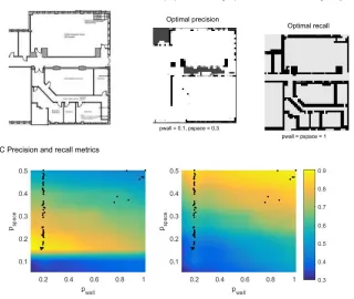
values too close to 1, were examined and linear interpolation was used to pro-duce continuous values. Figure 3C shows colour maps of the precision and

Figure 3A. Figure 3B shows the final maps produced using the prior values that yield maximum precision and those that yield maximum recall.

A higher precision ensures that it is unlikely free space will be incorrectly identified as occupied and a higher recall ensures that the building structure is detected. Figure 3C shows that the aims of having high precision and also maintaining a high recall are conflicting since pairs that yield high precision tend to yield low recall and vice versa. This problem of determining a suitable

pair of (pwall, pspace) that ensures high precision and high recall (> 40% was

empirically determined to be an appropriate threshold) is therefore a multi-objective optimisation problem.

In order to perform this multi-objective optimisation a controlled elitist ge-netic algorithm (Deb 2001) (a variant of NSGA-II (Deb et al. 2002)) was used. The Pareto front for the drawing in Figure 3A can be seen in Figure 3C and the final map produced using one of the Pareto optimal prior values is shown in Figure 3E. This drawing was chosen because, due to the level of detail includ-ing labelinclud-ing, walls at an angle and multiple rooms, it highlights the qualitative difference in performance between Figure 3B and Figure 3E.

The map shown in Figure 3E avoids detecting thicker walls or missing doors as can happen using the prior values that optimise recall, Figure 3B, and also avoids missing most of the walls as is done using the prior values that yield maximum precision, Figure 3B.

5.2

Multi-objective optimisation to determine globally

op-timal contextual priors

Figure 4B shows the precision and recall colour maps for all representative drawings in Figure 4A. The shape of the colour maps for precision and recall does not vary greatly between drawings, other than the fact that the region of values that yield good performance is larger/smaller for different drawings.

These results indicate that a globally optimal region of (pwall, pspace) values

that result in high precision can be identified.

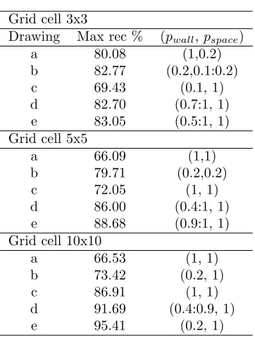
The locations of maximum precision for three different grid resolutions are

shown in Table 1. Maximum values are consistently observed forpwallvalues

be-tween 0.1 and 0.3 andpspace= 0.3 regardless of the drawing and grid resolution

with the exception of drawing (a) for a 10x10 grid cell.

The values that yield optimal recall can be seen in Table 2. These values are in most cases what one would intuitively expect to be optimal: a high value for pspace and a lower value for pwall. For the architectural drawing sections,

optimised values were found to be pspace = 1 with pwall between 0.1 and 1.

Both recall and precision are important to ensure a high quality map.

Figure 3: Multi-objective optimisation overview: A is the architectural draw-ing used to extract prior information; B shows the maps produced usdraw-ing prior values that yield maximum precision and maximum recall, neither of which is

qualitatively optimal; C shows thepreandreccolour maps for all combinations

of (pwall, pspace) between 0.1 and 1, with Pareto optimal values shown as black

points; D shows the Pareto front produced by the multi-objective otpimisation and E shows the map produced using the Pareto optimal proposed prior values

A B

1 1.5 2 2.5 3

1/precision 0 10 20 30 40 50 1/recall drawing (a) drawing (b) drawing (c) drawing (d) drawing (e)

0 0.2 0.4 0.6 0.8 1

pwall 0.1 0.2 0.3 0.4 0.5 0.6 0.7 0.8 0.9 pspace drawing (a) drawing (b) drawing (c) drawing (d) drawing (e)

0 0.2 0.4 0.6 0.8 1

pwall 0.1 0.2 0.3 0.4 0.5 0.6 0.7 0.8 0.9 pspace Cluster1 Cluster2 Cluster3

C D E

Figure 4: Multi-objective optimisation results for all drawings: A Drawings used to extract prior information; B Interpolated precision and recall colour maps for the five drawings; C Pareto fronts for all drawings, with a number of common solutions across drawings meaning there is a set of Pareto optimal (pwall, pspace) pairs that yield good performance for all drawings; D Pareto

optimal (pspace,pwalls) pairs plotted for all drawings; E Clusters detected within

Grid cell 3x3

Drawing Max pre % (pwall,pspace)

a 98.49 (0.3, 0.3)

b 99.42 (0.3, 0.3)

c 91.77 (0.3, 0.3)

d 95.56 (0.1, 0.3)

e 93.77 (0.3, 0.3)

Grid cell 5x5

a 75.00 (0.3, 0.3)

b 95.36 (0.3, 0.3)

c 79.00 (0.3, 0.3)

d 84.94 (0.1, 0.3)

e 90.51 (0.1, 0.3)

Grid cell 10x10

a 48.00 (0.5, 0.6)

b 89.14 (0.1, 0.3)

c 77.42 (0.1:0.2, 0.3:05)

d 92.06 (0.1, 0.3)

e 92.68 (0.1, 0.3)

Table 1: Maximum precision calculated for each of the drawings in Figure 4, grid cell size given in number of map pixels.

Multi-objective optimisation using the controlled elitist genetic algorithm (Deb 2001) (a variant of NSGA-II (Deb et al. 2002)) discussed in Section 5.1 was performed for all five drawings. Figure 4B shows the precision and recall interpolated colour maps for the five drawings used to generate the Pareto fronts in Figure 4C. Figure 4C shows the Pareto optimal fronts for all drawings and floor plans. There is a region where the Pareto optimal fronts for all drawings

overlap, meaning there are Pareto optimal sets of (pwall, pspace) values that yield

good performance regardless of the type of drawing used. Only solutions that

fall within setC as defined in Section 3.3 are of interest.

In the precision plots of Figure 4B we observe higher values forpwall= 0.2.

That is because 0.2 is the lowest probability value for which the log odds value is in the linear section of the log odds plot, Figure 5. Therefore it is the lowest value we can assign to detected walls that avoids the region close to the asymptote near 0.

In Tables 1 and 2 lower prior values for both pwall andpspace do not yield

optimal recall. This seems counter-intuitive given that assigning all cells a low prior probability would be expected to yield a low precision but high recall.

However, lowpwallandpspace can result in assigning high probabilities of being

empty to grid cells that contain mostly occupied space.

Using equation 5, for low pwall andpspace, if a cell contains both occupied

Grid cell 3x3

Drawing Max rec % (pwall,pspace)

a 80.08 (1,0.2)

b 82.77 (0.2,0.1:0.2)

c 69.43 (0.1, 1)

d 82.70 (0.7:1, 1)

e 83.05 (0.5:1, 1)

Grid cell 5x5

a 66.09 (1,1)

b 79.71 (0.2,0.2)

c 72.05 (1, 1)

d 86.00 (0.4:1, 1)

e 88.68 (0.9:1, 1)

Grid cell 10x10

a 66.53 (1, 1)

b 73.42 (0.2, 1)

c 86.91 (1, 1)

d 91.69 (0.4:0.9, 1)

e 95.41 (0.2, 1)

Table 2: Maximum recall calculated for each of the drawings in Figure 4, grid cell size given in number of map pixels.

InverseSensorM odel(mi,xk,zk) =

logOdds(0.9×pelempty

Ncell

) (10)

where pelempty are the number of pixels corresponding to detected empty

space in a given cell andNcellthe number of map pixels in a grid cell. A low prior

pspace <0.2 would result inl0,i <−1.4. For a cell containing fewer than 70%

pixels, corresponding to detected occupied spaceInverseSensorM odel(mi,xk,zk)>

0.4. Therefore, using equation 5, lk,i >2×(k−1)×2.8, which corresponds to

a probability greater than 0.94, incorrectly mapping this as an empty cell.

The Pareto optimal solutions for all drawings were plotted as shown in Fig-ure 4D. The k-means clustering method (Hartigan & Wong 1979), (Arthur & Vassilvitskii 2007) was then used to assign each point to clusters and the results are shown in Figure 4E.

In order to identify an optimal cluster of solutions, representatives from each cluster were tested in terms of qualitative performance. Solutions in Cluster 2,

the light blue cluster in Figure 4E, have high values of bothpwall and pspace.

Figure 5: The log odds plot for probability values 0-1. In the region 0.2-0.8 the log odds show linear behaviour, whereas for values outside that range the resulting log odds value increases rapidly

Figure 4E have low values of bothpwall and pspace and thus correspond to the

maximum precision solutions as shown in Table 1. These were also shown to produce non-optimal qualitative results as discussed in Section 5.1 and shown in Figure 3B. Therefore the optimal solution lies in Cluster 3, the green cluster. The values in the green cluster are those that intuitively would be expected

to perform well: a lowpwalland a highpspace. Converting these back to discrete

values, the possible solutions to investigate are the pairs

Shortlist=

(

pwall= 0.2, 0.6≤pspace≤1

0.4≤pwall≤0.5, 0.7≤pspace≤0.8

(11)

The maps produced using each of these pairs were compared in terms of

visual quality and the best (pwall, pspace) combination out of the green cluster

points in terms of qualitative performance was found to bepwall= 0.2,pspace =

0.9, Figure 6. The next sections discuss the benefits of using an informative

prior and compare the maps produced using the proposed informative prior to those produced using an uninformative prior to quantify the improvement in performance.

5.3

Effects of sensor model on optimised prior values

The proposed optimised prior values were obtained for an optimisation using the simple sensor model described in Section 4.2. The effect of selecting different sensor models is explored in this section. Different sensor models assign a

differ-ent probability of occupancy to detected free and occupied space, settingpf ree

to detected empty space cells and poccupied to cells corresponding to occupied

space. More complex models might use a normal distribution centred around

the location of a detected obstacle/detected empty space cell forpoccupied and

pf ree (Pirker, R¨uther, Bischof & Schweighofer 2011).

initialisa-C D

Figure 6: Comparison of map produced using the proposed optimised prior and the map produced using a informative prior: A Maps produced using a non-informative prior for two different grid resolutions; B Processing and converting a drawing to an optimised prior and using it to produce maps for two different grid resolutions; C A quantitative comparison of the maps produced using an

informative and a non-informative prior using theF2metric; D Evolution ofF2

tion oflk,i=l0,i. Using equation 5, this leads to the update rule

l1,i=InverseSensorM odel(mi,x1,z1)

l2,i= 2×_{InverseSensorM odel}(m_i,x2,z2)−l0,i ..

.

l_k,i=k×_{InverseSensorM odel}(m_i,x_k,z_k)−(_k−1)×l0,i

(12)

for theith cell at the kth iteration. Therefore, to obtain a larger final map

probability for empty cells we need lk,i > 0 corresponding to a probability of

occupancypk

mi>0.5, Figure 5. lk,i>0 would require

InverseSensorM odel(mi,xk,zk)>l0,i (13)

for a large k. Therefore the probability assigned by the sensor model to

detected free space should be greater than the prior value assigned to empty

spacepf ree> pspace. Conversely, the value assigned to detected occupied space

by the sensor model should be smaller than the prior,poccupied< pwall.

5.4

Benefits of using an optimised informative prior

Using an optimised informative prior allows for improved performance when a robot quickly explores an area while operating in a time-critical mission such as USAR, for example. In the mapping example presented in Figure 6 the robot has not fully explored the environment. In such cases using a prior has the added benefit of providing information about building sections even if areas are unexplored. Moreover, for coarse grid resolutions the commonly used uninfor-mative prior produces maps of very low quality whereas the proposed optimised

prior ofpwall= 0.2,pspace= 0.9 produces maps that give an overview of

build-ing structure, as shown in Figure 6. Therefore if a quick and computationally cheaper exploration is required the proposed optimised prior yields significantly better maps in terms of visual quality, identifying the majority of building walls. The maps produced using the proposed prior perform better in a quanti-tative sense as shown in Figure 6C. Given the multi-objective nature of the optimisation, merely comparing the values of precision and recall for maps pro-duced using the informative and non-informative prior does not provide enough

information. In order to overcome this problem theF2 metric (Powers 2011) is

used to allow a comparison of the precision and recall combination rather than individual values for each drawing.

F2= 5×

pre×re

(4×pre) +rec (14)

Recall is favoured over precision since it represents the percentage of cor-rectly detected walls and thus affects the map outline more. As shown in

Fig-ure 6C using an informative prior yields an increase inF2 measure of at least

20% over the uninformative prior. Moreover, it is worth noting that using an

of exploration (Figure 6D) greatly outperforming the map produced using the non-informative prior.

The overall method proposed in this paper to process an architectural draw-ing or floor plan, extract structural information and use it to construct an optimised prior and thus an improved map is shown in Figure 6B.

6

Experimental results

In order to verify the results obtained using simulated data, distance data were collected using a turtlebot mounted with a Microsoft Kinect sensor running ROS. Two sets of experiments were conducted

• A small scale experiment in a constructed course, aiming to simulate a

building, Figure 7A. The robot pose was measured perfectly by hand.

• A large scale experiment in a floor of a University of Sheffield Engineering

building. In this case we used Adaptive Monte Carlo Localisation and the extracted prior to produce estimates of the robot pose.

In both cases the occupancy grid Matlab code presented in Section 4.2 was used to update the map.

6.1

Constructed robot course

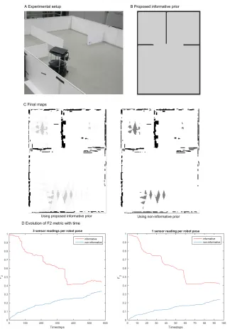
A known, accurate robot pose was used at each time step and the occupancy grid map update in the Matlab simulator proposed in Section 4.2 was used to process the data collected using the Kinect sensor.

An informative prior map produced using perfectly extracted walls and

as-signing the proposed prior values pwall = 0.2, pspace = 0.9 was used,

Fig-ure 7B. The maps produced using the proposed informative prior and the non-informative prior are shown in Figure 7C for an exploration that takes 3 sensor readings per robot pose. The exploration is incomplete with unexplored areas shown in grey. Grey areas in the map that uses the proposed prior correspond to a probability of 0.9 and in the map produced using the non-informative prior to 0.5, providing no information about the environment. This is an advantage of using the proposed prior since, even if areas remain unexplored, there is some information about what we expect to find there. The map that uses the pro-posed prior has correctly detected walls at the bottom of the image as well as the outer right wall. Conversely, using the non-informative prior has resulted in poorly detected outer walls and multiple grey areas that provide no information about the environment.

Figure 7D shows a comparison of the evolution of the F2 metric with time

when using the proposed informative prior and the non-informative prior when 3 sensor readings are used per pose and when only 1 reading is used per pose. These results agree with the simulation results, with the proposed method

Figure 7: Experimental setup and results. A Experimental setup and robot used; B Accurate prior map of the environment; C Final maps produced using the proposed informative prior (left) and the non-informative prior (right); D

Evolution of theF2 metric with time for an exploration that takes 3

Note that the starting F2 value for the maps produced using the informative

prior is very high because the prior used is very accurate and drops as less accu-rate sensor readings are incorpoaccu-rated. Even if the prior information is extracted accurately the final map should be updated using sensor information since floor plans may be outdated (for example due to a demolished wall) or no longer accurate (due to a collapsed wall in a USAR environment).

The multi-objective optimisation proposed in Section 3.3 was repeated for a more realistic sensor model and using the real Kinect data collected during the experiment. The following model was used, based on (Pirker et al. 2011)

InverseSensorM odel(mi,xk,zk) =

        

0.9, npixels<z_i =npixels_i

0.1, npixels>zi =n pixels i

npixels<zi

npixelsi

, 0< npixels<zi < n pixels i

(15)

withnpixels<zi being the number of map pixels for a celli that fall between

the robot and the location of the detected obstacle, z, npixels>zi the number

of map pixels for a cellithat are located beyond the detected object or at the

location of the detected object andnpixelsi the number of map pixels in celli. For

an accurate sensor, cells for which all map pixels correspond to detected empty space are assigned a value of 0.9, those that correspond to detected objects a value of 0.1 and those that contain both empty space and objects are assigned a value equal to the percentage of pixels corresponding to detected objects.

A very narrow range of optimal (pwall, pspace) was observed, which mostly

agree with the results obtained in simulation, yielding opimised values ofpwall=

0.2 and pspace = 1. These values are multiplied by a factor of 0.9 before they

are used in the prior map as explained in Section 5.1 to avoid values too close to 1. A less accurate sensor model assigning 0.8 to detected empty space and

0.2 to detected walls was also tested, yielding optimised valuespwall= 0.4 and

pspace= 0.75.

6.2

Larger scale experimental results

prior map: more accurate localisation and the ability to start with a known,

accuratex0.

The walls used to construct the prior map in this case, Figure 8A are not perfectly extracted, with some of the doors appearing as wall sections on the 6th room in the top row and the 5th room in the bottom row of offices. The final map is unaffected by these small inaccuracies which are corrected during mapping.

Some experiments were also run using a less accurate x0, using particles

initialised with a non-zero variance. The resulting maps were less accurate but still better than those proposed using a non-informative prior. For a low variance

the results were very similar to those produced using a perfectly accuratex0.

Assuming a known prior pose is realistic since, given the extracted prior and a floor plan an operator can align the robot to a known location before starting exploration.

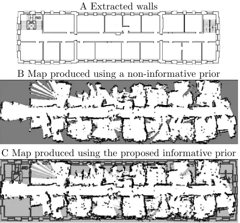
The results of these experiments are shown in Figure 8. Using the proposed prior yields a more accurate map both in a qualitative and quantitative sense.

The map produced using the proposed prior yields a higher F2 value, even if

parts of the building are unexplored. It also yields more correctly mapped walls, demonstrating the advantages of using the proposed prior over a non-informative one. These results also demonstrate an added benefit of using a prior map. If exploration of the whole floor were not possible due to, for example, limited exploration time in a time-critical mission or certain areas being inaccessible, the proposed prior provides some information about unexplored areas. This may not be completely accurate but it would allow a human operator or rescuer to better interpret the mapped sections.

The map shown in Figure 8B is less easy to interpret: it is unclear what sections of the building the map areas correspond to and many of the walls have not been mapped correctly. Conversely, using the proposed informative prior, Figure 8C, a human can interpret the map more easily. Moreover the majority of corridor walls have been mapped correctly, unlike Figure 8B where many of them are mapped as empty space.

In all cases there appears to be some noise in the map, particularly within the detected rooms. That is due to the fact that the environment explored was a real world, cluttered office building, containing furniture. Therefore objects detected within the rooms mostly correspond to desks, chairs, bookcases and half-open doors. Since our aim is to improve performance in real world environments we did not aim to simplify the environment by only exploring long corridors (as is often done in the literature) or emptying the rooms.

A Extracted walls

B Map produced using a non-informative prior

C Map produced using the proposed informative prior

D Map produced using the proposed informative prior;x0 with a variance of

0.1 (less accurate initial pose)

E Evolution ofF2 with time

Figure 8: Large scale experimental results. A Prior map of extracted walls and empty space of Floor C of the Amy Johnson building, Dept of Automatic Control and Systems Engineering, University of Sheffield; B Map produced using a non-informative prior; C Map produced using the proposed prior, successfully mapping more walls than using the non-informative prior; D Map produced

using the proposed informative prior and a slightly less accuratex0; E Evolution

7

Conclusions

This paper presents a method to construct optimised indoors occupancy grid mapping priors. Priors were constructed using structural information extracted from architectural drawings and floor plans by assigning appropriate prior prob-abilities to detected wall and empty space locations. A precision-recall analysis was used to assess quantitative performance and a multi-objective optimisation was used to short list Pareto optimal solutions. Both types of drawings were

found to have a similar region of (pwall, pspace) that yields good performance

metrics.

The commonly used uninformative prior was found to perform worse than a prior constructed using an architectural drawing and was not one of the Pareto

optimal solutions. The values pwall = 0.2, pspace = 0.9 were found to yield

optimal results in terms of qualitative performance whilst also yielding an

im-provement inF2metric of over 20%.

The main contribution of this paper is thus a method to produce optimised Bayesian priors that improve map quality in indoors SLAM applications without adding to the computational complexity of the SLAM algorithm itself. There is a one-off cost of extracting the prior value but no further increase in compu-tational complexity. This method also yields improved performance compared to the non-informative prior for coarser grids or explorations that do not cover the entire building. It is therefore very well suited to time critical challenging real life applications such as USAR missions where a fast and accurate SLAM implementation is required.

Acknowledgments

We would like to thank Jon Lipsky, lead developer of Elevenworks LLC, for allowing us to use a floor plan featured in the Elevenwork website, Figure 3 drawing (a) and the University of West Florida for allowing us to use an image of a floor plan of the Heritage Halls of residence, Figure 3 drawing (b) to test the mapping algorithms presented in this paper.

Funding

The research presented in this paper was funded by the University of Sheffield and PA Consulting.

Appendix: Occupancy grid mapping

p(m|X0:k,Z0:k) =

Y

i

p(mi|X0:k,Z0:k) ₍₁₆₎

where i = 1, ..., N is the current grid cell and N the total number of grid

cells, making this an easier estimation since updating the probability for each cell given the robot pose and sensor readings is merely an update of the probability of occupancy of that cell. As the robot moves through the environment the probabilities of occupancy of cells that are within the field of view of the robot sensors are updated.

The probability that a cellmi is occupied given the observation history is

given by

p(mi|Z0:k) =

p(zk|mi,Z0:k₋1)p(mi|Z0:k₋1)

p(zk|Z0:k−1)

(17)

which can be written as

p(mi|Z0:k) =p(zk|mi)

p(mi|Z0:k−1)

p(zk|Z0:k₋1)

(18)

using the static world assumption which states that past sensor readings are

conditionally independent given knowledge of the mapm(Thrun 2003). Thus

Equation 18 can be written as

p(mi|Z0:k) =

p(mi|zk)p(zk)

p(mi)

p(mi|Z0:k₋1)

p(zk|Z0:k−1)

(19)

usingp(zk|mi) =

p(mi|zk)p(zk)

p(mi)

.

Placing Equation 19 in the odds form we get

odds(mi|Z0:k) =

p(mi|Z0:k)

p(¬mi|Z0:k)

= p(mi|zk)p(mi|Z1:k−1)p(¬mi)

p(¬mi|zk)p(¬mi|Z1:k₋1)p(mi)

(20)

Therefore

odds(mi|Z0:k) =

odds(mi|zk)odds(mi|Z1:k−1)(odds(mi))

−1 (21)

wherep(mi) is the prior probability of occupancy of theith grid cell,odds(mi|Z1:k₋1)

is the odds at the previous time step andodds(mi|zk) represents the inverse

sen-sor model. Taking the logarithm of Equation 21, the log odds representation of Equation 21 is

with

lk,i=log

p(mi|Z1:k,x1:k)

1−p(mi|Z1:k,x1:k)

(23)

Methods to select a suitable or preferable inverse sensor model are proposed in (Thrun 2003) and (Yaqub & Katupitiya 2007).

References

Arthur, D. & Vassilvitskii, S. (2007), k-means++: The advantages of careful

seeding, in ‘Proceedings of the 18th Annual ACM-SIAM Symposium on

Discrete algorithms’, pp. 1027–1035.

Baden-Powell, C., Hetreed, J. & Ross, A. (2011), Architect’s Pocket Book,

El-sevier.

Barnes, D., Maddern, W. & Posner, I. (2015), Exploiting 3D Semantic Scene

Priors for Online Traffic Light Interpretation,in‘Proceedings of the IEEE

Intelligent Vehicles Symposium’.

Burschka, D., Geiman, J. & Hager, G. (2003), Optimal landmark configuration

for vision-based control of mobile robots,in‘Proceedings of the IEEE

Inter-national Conference on Robotics and Automation’, Vol. 3, pp. 3917–3922 vol.3.

Collins, T., Collins, J. & Ryan, C. (2007), Occupancy Grid Mapping: An

Em-pirical Evaluation, in‘Proceedings of the 15th Mediterranean Conference

on Control and Automation’.

Davis, J. & Goadrich, M. (2006), The relationship between Precision-Recall

and ROC curves,in‘Proceedings of the 23rd International Conference on

Machine Learning’, ACM Press, pp. 233–240.

de la Puente, P. & Rodriguez-Losada, D. (2014), ‘Feature based graph-SLAM

in structured environments’,Autonomous Robots 37(3), 243–260.

Deb, K. (2001), Multi-objective optimization using evolutionary algorithms,

Vol. 16, Wiley Interscience Series in Systems and Optimization.

Deb, K., Pratap, A., Agarwal, S. & Meyarivan, T. (2002), ‘A fast and elitist

multiobjective genetic algorithm: NSGA-II’,IEEE Transactions on

Evolu-tionary Computation6(2), 182–197.

Dissanayake, M., Newman, P., Clark, S., Durrant-Whyte, H. & Csorba, M. (2001), ‘A solution to the Simultaneous Localization And Map

build-ing (SLAM) problem’, IEEE Transactions on Robotics and Automation

17(3), 229–241.

Durrant-Whyte, H. & Bailey, T. (2006), ‘Simultaneous Localization and

Elfes, A. (1989), ‘Using occupancy grids for mobile robot perception and

navi-gation’,Computer22(6), 46–57.

Georgiou, C., Anderson, S. & Dodd, T. (2015), Constructing contextual SLAM

priors using architectural drawings, in ‘Proceedings of the International

Conference on Automation, Robotics and Applications’, pp. 50–56.

Giagkiozis, I., Purshouse, R. C. & Fleming, P. J. (2015), ‘An overview of

population-based algorithms for multi-objective optimisation’,

Interna-tional Journal of Systems Science 46(9), 1572–1599.

Grewe, R., Komar, M., Hohm, A., Lueke, S. & Winner, H. (2012), Evaluation

method and results for the accuracy of an automotive occupancy grid, in

‘Proceedings of the IEEE International Conference on Vehicular Electronics and Safety’, pp. 19–24.

Hartigan, J. A. & Wong, M. A. (1979), ‘Algorithm AS 136: A K-Means

Cluster-ing Algorithm’,Journal of the Royal Statistical Society. Series C (Applied

Statistics)28(1), pp. 100–108.

Kumar, V., Rus, D. & Singh, S. (2004), ‘Robot and Sensor Networks for First

Responders’,IEEE Pervasive Computing3(4), 24–33.

Maddern, W., Pascoe, G. & Newman, P. (2015), Leveraging Experience for

Large-Scale LIDAR Localisation in Changing Cities,in‘Proceedings of the

IEEE International Conference on Robotics and Automation’.

Mazuran, M., Tipaldi, G. D. & Stachniss, C. (2014), A Statistical Measure

for Map Consistency in SLAM,in‘Proceedings of the IEEE International

Conference on Robotics and Automation’, pp. 3650–3655.

Milstein, A. (2005), Occupancy Grid Maps for Localization and Mapping, in

X.-J. Jing, ed., ‘Motion Planning’, InTech, chapter 19, pp. 381–408.

Montemerlo, M., Thrun, S., Koller, D. & Wegbreit, B. (2003), FastSLAM 2.0: An Improved Particle Filtering Algorithm for Simultaneous Localization

and Mapping that Provably Converges,in‘Proceedings of the International

Joint Conferences on Artificial Intelligence’.

Parsley, M. & Julier, S. (2011), Exploiting prior information in GraphSLAM,

in ‘Proceedings of the IEEE International Conference on Robotics and

Automation’, pp. 2638–2643.

Pirker, K., R¨uther, M., Bischof, H. & Schweighofer, G. (2011), Fast and accurate

environment modeling using three-dimensional occupancy grids, pp. 1134– 1140.

Powers, D. M. W. (2011), ‘Evaluation: From Precision, Recall and F-Measure

to ROC., Informedness, Markedness & Correlation’, Journal of Machine

Thrun, S. (2003), ‘Learning Occupancy Grid Maps With Forward Sensor

Mod-els’,Autonomous Robots15(2), 111–127.

Williams, B. & Reid, I. (2010), On combining visual SLAM and visual odometry,

in ‘Proceedings of the IEEE International Conference on Robotics and

Automation’, pp. 3494–3500.

Yaqub, T. & Katupitiya, J. (2007), Laser scan matching for measurement

up-date in a particle filter, in‘Proceedings of the IEEE/ASME International