Subspace Tracking Based Blind MIMO Transmit
Preprocessing
W. Liu, L. L. Yang and L. Hanzo
School of ECS, University of Southampton, SO17 1BJ, United Kingdom.
Tel: +44-23-8059 6671, Fax: +44-23-8059 4508
Email:
{
wl03r,lly,lh
}
@ecs.soton.ac.uk, http://www-mobile.ecs.soton.ac.uk
Abstract— In this contribution projection approximation
sub-space tracking using deflation (PASTD) is investigated in the context of MIMO transmit preprocessing systems by exploiting the specific property of Time Division Duplexing (TDD) tech-niques that the uplink and downlink channels are similar, since they both use the same carrier frequency. Hence the channel estimated from the received signal can also be used for transmit preprocessing. More explicitly, based on the received signal, the PASTD algorithm is used for tracking both the left and the right singular vectors of the MIMO channel matrix, which are required by eigenmode transmissions, instead of periodically reestimating the MIMO channel matrix and performing the singular value decomposition (SVD), which would impose a high computational complexity. A specific deficiency of the family of subspace tracking algorithms is their phase ambiguity imposed by the the non-unique nature of the SVD, which is resolved in this treatise by employing differential encoding. The efficiency of the proposed subspace tracking scheme is demonstrated by our performance results, indicating that the advocated technique preforms within 1dB from the BER curve of the perfect channel estimation aided benchmarker.
I. INTRODUCTION
Due to the emerging high demand for supporting novel multimedia applications, next generation wireless systems are expected to support higher data rates. When employing multi-ple antennas at both the transmitter and receiver, multimulti-ple input multiple output (MIMO) systems have the potential achieving a high transmission rate than their traditional single input single output (SISO) counterparts [1].
MIMO systems have attracted intensive research interests during the last decade [1]–[3]. In the absence of channel state information (CSI) at the transmitter, space time coding [4] or spatial multiplexing [5], [6] constitue prime candidates for MIMO transmission. However, when the CSI is available at both the transmitter and the receiver, a more sophisticated technique refered to as eigenmode transmission [7] can be used for decomposing the MIMO channel into several independent SISO subchannels, which involves the singular value decom-position (SVD) of the MIMO channel matrix. In this case no joint detection is needed and the resultant single-antenna-based detection algorithm becomes rather simple.
The third-generation (3G) wireless systems support two different modes, namely frequency division duplexing (FDD) and time division duplexing (TDD) [8], [9]. In the FDD mode, the uplink (UL) and downlink (DL) signals are transmitted at
The financial support of the European Union under the auspices of the Newcom and Phoenix projects, as well as that of the EPSRC UK is gratefully acknowledged.
different carrier frequencies, which results in independently fading channels for the UL and DL. By contrast, in the TDD mode, the UL and DL transmissions ensue at the same carrier frequency. Hence the UL and DL channels tend to fade together and therefore can be considered as similar [8]. We will exploit this similarity of the UL and DL channels of the TDD mode in this paper.
The CSI required at the transmitter can be obtained with the aid of the side-information control channel from the receiver in the FDD mode. Alternatively, it can be directly estimated on the basis of the received signal’s quality and exploited by the transmitter in the TDD mode.
Channel estimation (CE) followed by singular value de-composion (SVD) is invoked, when eigenmode transmissions are employed [10], which potentially imposes a high com-putational complexiy. Instead of estimating the entire MIMO channel matrix and then additionally implementing SVD, it was claimed in [11], [12] that subspace tracking based algorithms may result in lower computational complexity in the context of eigenmode transmissions.
In the family of subspace tracking algorithms, the so-called projection approximation tracking combined with deflation (PASTD) [13] has been shown to be applicable in diverse scenarios [14], [15]. Hence, in this paper PASTD algorithm is employed for subspace tracking in a MIMO-aided TDD system.
II. MIMO TRANSMISSIONMODEL
Consider a system havingMT transmitter andMRreceiver
antennas subjected to a flat-fading channel between any pair of transmitter and receiver antennas. Then the receivedMR
-dimensional symbol vectorycan be expressed as
y = Hx+n, (1)
where x is the MT-dimensional transmitted symbol vector
and H is an (MR × MT)-dimensional complex channel
matrix with the (i, j)th element being the fading channel between the ith receive and jth transmit antennas. Finally,
nis theMR-dimensional AWGN vector having a zero-mean
andE(nnH) =σ2
nIMR. HereIM is an(M×M)-dimensional identity matrix.
If the rank ofHis assumed to beq(q≤min(M, N)), the SVD of the channel matrixH is given by
H = UΛVH
= [Us Un]
Λs 0
0 0
VH s VH
n
where U is an (MR×MR)-dimensional unitary matrix
sat-isfying UHU=I
MR and Vis an (MT ×MT)-dimensional unitary matrix having the property ofVHV=I
MT, whileΛ is an(MR×MT)-dimensional matrix andIM is an(M×M)
-dimensional identity matrix. In the second line of (2), Λs
is a (q ×q)-dimensional diagonal matrix having diagonal elements of λ1 ≥λ2· · ·λq−1 ≥ λq, which are the singular
values of H. Furthermore, in (2) we portrayed U and V
in form of two components, where Us is an (MR ×q)
-dimensional matrix constituted by the first p columns of U, which span the column-space of H andVs is an(MT ×p)
-dimensional matrix formed by the firstqcolumns ofV, which span the row-space of H. Still referring to (2), Un is an [MR×(MR−q)]-dimensional matrix, which is orthogonal
to Us, while spanning the null space of H and Vn is an [MT×(MT−q)]-dimensional matrix that is orthogonal toVs
and spans the left null space of H.
If the channel matrix H is known at both the transmitter and receiver, the so-called eigenmode transmission regime of [7] can be invoked to decompose the MIMO channel into orthogonal subchannels by applying Vs and Us at the
transmitter and receiver, respectively, yielding
˜
y = UHs y
= UHs (HVs˜x+n)
= Λ˜x+˜n, (3)
where ˜xis a q-dimensional transmitted symbol vector, while
˜
n = UHs n is a q-dimensional noise vector, which has the
same statistical properties asn(dl,k), becauseUHs is a unitary
matrix.
As an explicit benefit of using the SVD, the known channel matrixHis finally decomposed intoqindependent orthogonal subchannels, each of which has a channel gain of λi and
this transmit preprocessing regime is referred to as eigenmode transmission [7].
As a further simplication, it was shown in [11] that high-integrity reception can be achieved, if we opt for transmitting in a limited number of p (1 ≤ p ≤ q) subchannels having channel gains of λ1 ≥ λ2· · · ≥ λp for achieving a high
throughput, while meeting the specific target BER perfor-mance.
Another potential advantage of eigenmode transmission is that only the left singular vectors of Us and the right
singular vectors of Vs are needed, as we can see in (3).
Hence it is intuitively appealing to invoke algorithms, which estimate or update the singular vectors only [11], [12] instead of estimating the entire MIMO channel matrix H and then additionally implementing the SVD, which would inevitably impose a high computational complexity.
III. TDD MIMO TRANSMISSIONMODEL
A full-duplex MIMO link may be created using either FDD or TDD mode. In this paper, we assume employing the TDD mode. Consider a TDD system using MT antennas at the
base station (BS) and MR antennas at the mobile station
(MS), encountering a flat-fading channel between any pair of transmitter and receiver antennas. Furthermore, for simplicity,
we assume that the system supports a single user. Then the MR-dimensional received symbol vectorydl(k)of the DL and
theMT-dimensional received symbol vectoryul(k)of the UL
can be expressed as
ydl(k) = Hdl(k)xdl(k) +ndl(k), (4)
yul(k) = Hul(k)xul(k) +nul(k), (5)
wherexdl(k)is anMT-dimensional DL symbol vector
trans-mitted from the BS to the MS, while xul(k) is an MR
-dimensional UL symbol vector transmitted from the MS to the BS. Furthermore,Hdl(k)is the DL channel matrix andHul(k)
is the UL channel matrix. Moreover,ndl(k)is the DL AWGN
noise vector having a zero-mean andE(ndlnHdl) =σ2ndlIMR,
nul(k)is the UL AWGN noise vector having a zero-mean and
E(nulnHul) =σn2ulIMT.
Since the UL and DL timeslots of a TDD link are trans-mitted on the same carrier frequency, the UL and DL channel matrices may be assumed to be identical, provided that the Doppler frequency is sufficiently low and hence the corre-sponding channel impulse response (CIR) does not change dramatically during the time between the UL and DL time slot. Hence we have
Hul(k) = HTdl(k). (6)
Upon substituting (6) into (5), we arrive at
yul(k) = HTdl(k)xul(k) +nul(k). (7)
The transmitted symbol vectorxulis conjugated before
trans-mission, as proposed in [11]. In this case, we obtain
yul(k) = HTdl(k)x∗ul(k) +nul(k). (8)
Furthermore, the received symbol vector is conjugated as well, hence we have
y∗
ul(k) = H
H
dl(k)xul(k) +n∗ul(k). (9)
According to (2), the SVD ofHdl can be expressed as
Hdl = [Udls Udln]
Λdls 0
0 0
VH dls
VH dln
, (10)
whereUdls is an(MR×q)-dimensional unitary matrix, while
Vdls is an(MT×q)-dimensional unitary matrix. Furthermore,
Λdlsis a(q×q)-dimensional diagonal matrix with its diagonal elements given by λ1 ≥ λ2· · ·λq−1 ≥ λq, which are the
singular values ofHdl. Accordingly, the SVD ofHHis given
by
HHdl = [Vdls Vdln]
Λdls 0
0 0
UHdl
s
UH dln
. (11)
When eigenmode transmission is used for the sake of avoiding interference among the transmitted data symbols, thep-dimensional transmitted symbol vectors˜xdland˜xulare
multiplied by Vdlsp andUdlsp given by the first p columns of Vdls and Udls, respectively, before their transmission. Accoding to (3), we obtain
y∗
ul(k) = H
H
dl(k)Udlsp˜xul+nul(k). (13)
The resultant received symbol vectors ydl and yul∗ are
multiplied by the matrices UH
dlsp andV
H
dlsp, respectively, for the sake of avoiding interference among the transmitted data symbols. Finally, we obtain
˜
ydl(k) = UHdlsp(k)ydl(k)
= Λdlp(k)˜xdl(k) +U
H
dlsp(k)ndl(k), (14)
˜
yul(k) = VHdlsp(k)y ∗
ul(k) = Λdlp(k)˜xul(k) +V
H
dlsp(k)nul(k), (15)
where Λdlp is a (p×p)-dimensional diagonal matrix having
λ1 ≥ λ2· · ·λp−1 ≥λp as its diagonal elements. As we can
see, only the matrixUdlsp has to be known at the MS, while the matrixVdlsp is used for preprocessing at the BS.
The matrices Udlsp and Vdlsp can be obtained by SVD of the channel matrix Hdl. However, this requires estimating
the channel matrix first, then implementing the SVD, which improses a high computational complexity. Observe in (9) to (15) however, that only the subspace matricesUdlspandVdlsp are required instead of the knowledge of the entire channel matrix.
Let us continue by considering the DL transmission in more detail. More explicitly, our goal is to obtain the matrices
UdlspandVdlspwithout estimating the channel matrixHand without performing the SVD ofH. Upon substituting (10) into (12), we obtain
ydl = [Udls Udln]
Λdls 0
0 0
VdlH
s
VH dln
Vdlspx˜dl+ndl.
(16)
The autocorrelation matrix of the vector ydl of received
symbols is given by
Rydl=E[ydly
H
dl] =HdlVdlspR˜xdlV
H dlspH
H
dl+σn2dlI. (17)
Let the total average transmit powerP be a constant and let us allocate an equal power to each nonzero subchannel in (16). Then we obtain the autocorrelation of thep-dimensional vector
˜
xdl of transmitted symbols as follows
R˜xdl =E[x˜dlx˜
H dl] =
P
pIp. (18)
Hence, following a few further manipulations, (17) can be written as
Rydl = [Udls Udln]
P
pΛ
2
dlsp+σ 2
ndl 0
0 σn2dl
UH dls
UH dln
,
(19)
whereUdlsis constituted byqeigenvectors ofRydl associated with the q largest eigenvalues (P
pλ
2
1 +σ2ndl) ≥ (
P pλ
2 2 + σn2dl)· · · ≥ (
P pλ
2
q +σn2dl) of Rydl. The space spanned by the columns of Udls is referred to as the signal subspace, while Udln consists of (MR−q) number of eigenvectors of
Rydl related to (MR−q) number of eigenvalues {σ 2
ndl} of
Rydl. Finally, the space spanned by the columns of Udln is
Operation procedure of PASTD algorithm
y1(k) =ydl(k)
Fori= 1,2,· · ·, p, Do
ri(k) =wi(k−1)yi(k); prejection operation di(k) =βdi(k−1) +|ri|2;
ei(k) =yi(k)−wi(k−1)ri(k);
wi(k) =wi(k−1) +ei(k)[r∗i(k)/di(t)]; updating eigenvectors yi+1(k) =yi(k)−wi(k)ri(k); deflation
TABLE I
THEPASTDALGORITHM DESIGNED FOR TRACKING THE SIGNAL SUBSPACE COMPONENTS OF THE RECEIVED SIGNAL VECTORydl
termed as the noise subspace, which is orthogonal to the signal subspace [12], [14].
We can see from our discussions above that the eigenvectors in Udls also consist of the orthonormal basis vector of the column-space of Hdl. Moreover, when the vector ydl of
re-ceived symbols becomes available, so-called subspace tracking algorithms can be used to track the orthonormal basis vectors of Udlsp, which spans the column-space ofH.
Similarly, when the vector y∗
ul of received symbols
be-comes available, the eigenvectors in Vdlsp can be tracked as well, which spans the row-space of H. Upon obtaining the corresponding left and right singular vectors of H, the eigenmode MIMO-aided transmission regime described above can be employed.
In the family of different subspace tracking algorithms, the Projection Approximation Subspace Tracking technique using deflation (PASTD) [13] stands out as one of the most popular algorithms. In the next section, the PASTD algorithm will be briefly described in the context of tracking the elements of
Udlsp. The same algorithm can also be used for tracking the elements ofVdlsp.
IV. PASTD SUBSPACETRACKING[13]
The PASTD algorithm of [13] designed for signal sub-space tracking is summarized in Table I, where ydl(k) is
the kthMR-dimensional received signal vector generated for
DL transmission, while di(k) represents the exponentially
weighted estimate of the ith eigenvalue and wi(k) denotes
the estimate of the ith eigenvector at the kth time instant. Furthermore, β (0 < β ≤1) represents the forgetting factor. Table I summarizes the operations of the PASTD algorithm, which is based on the so-called deflation technique [13] and its basic philosophy is that of the sequential estimation of the so-called principal components [13]. The most dominant eigenvector is updated first by applying the PAST algorithm at the 1st iteration [13]. Then the projection of the current signal sample vectorydl(k)onto this eigenvector is removed
fromydl(k)itself. Now the second most dominant eigenvector
becomes the most dominant one in the updated signal vector and hence can be extracted in the same way as outlined above. This procedure is applied repeatedly, until all desired eigencomponents have been estimated.
Number of transmitter antennasMT 4 Number of receiver antennasMR 4 Normalized maximum Doppler frequencyfdmTs 0.001
[image:4.595.75.278.51.104.2]Forgetting factorβin Section IV 0.95 TABLE II
PARAMETERS FOR THEPASTDALGORITHM INTDDMODE
reorthogonalizing the signal subspace after each update. The variablesdi(0)andwi(0)have to be initialized, as seen
in Table I . Specifically, the SVD of the firstM vectors of the received symbols are used for the initialization of di(0) and wi(0)[14].
Since the singular vector generated according to (2) can be different up to a complex-valued coefficient of unit norm [11], it may cause phase ambiguity [11], which can be resolved for example by differential encoding, leading to differential phase shift keying (DPSK) modulation [11].
V. PERFORMANCERESULTS
Having described the TDD system and the PASTD algo-rithms in Section IV, in this section our simulation results are provided in order to characterize the attainable performance of PASTD subspace tracking in the context of a TDD system. Furthermore, differential BPSK modulation is used.
0.8 0.85 0.9 0.95 1.0 Forgetting factor
10-5 10-4 10-3 10-2 10-1 1
BER
[image:4.595.337.522.286.429.2]SNR=-10dB SNR=-5dB SNR=0dB
Fig. 1. BER performance against the forgetting factor β introduced in Section IV, when only the largest eigenvalue is used for uplink transmission at different values of SNR. The remaining parameters are the same as in Table II.
In Figure 1 the achievable BER performance is plotted against the forgetting factor β, when only the largest eigen-value is used for both the uplink and downlink transmissions, respectively, at SNRs of−10dB,−5dB and0dB. The remain-ing parameters are the same as in Table II. We can see from Figure 1 that for a given SNR, the BER slightly decreases upon increasing the forgetting factorβ, until an optimum point is reached. Beyond this point the BER increases relatively sharply upon increasing the forgetting factorβ. This is because for the low normalized Doppler frequency offdmTs= 0.001,
the channel exhibits a high correlation for a long period, which
allows us to exploit the channel knowledge over a longer period, resulting in a higher forgetting factor. Beyond the optimum value ofβ, more than necessary past channel output samples are invoked, therefore the correlation between a far distant channel sample and the current one is low and hence the effects of the noise imposed by a distant noisy sample on the correlation becomes more dominant, which actually degrades the algorithm’s performance. We can also see for SNR=−10dB and−5dB that the optimum forgetting factor is around β = 0.95, while for SNR=0dB it is around 0.90. The reason behind this may be attributed to the observation that for lower SNRs a higher number of noisy samples may be needed to mitigate the effects of the noise and hence a higher forgetting factor is required. By contrast, for higher SNRs a lower number of noisy samples is sufficient for mitigating the effects of noise, which results in a lower forgetting factorβ.
-10 -5 0 5 SNR (dB)
10-5 10-4 10-3 10-2 10-1 1
BER
UL Tracked UL Perfect
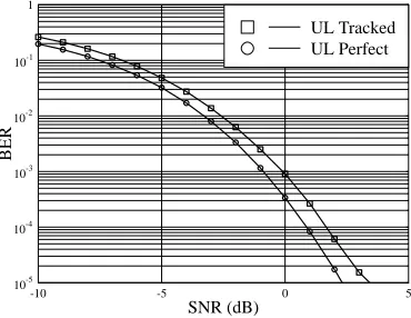
Fig. 2. BER versus SNR performance, when only the largest eigenvalue is used for uplink transmission. The remaining parameters are the same as in Table II.
In Figure 2 the attainable BER performance is portrayed for different values of the SNR, when only the largest eigenvalue is used for uplink transmission. The remaining parameters are the same as in Table II. We can see from Figure 2 that the achievable BER performance of PASTD subspace tracking is similar to that achieved with the aid of perfect channel knowledge. Observe, however that the BER difference between the perfect estimation based scenario and the tracked scenario becomes higher upon increasing the SNR. This is because the forgetting factor ofβ= 0.95is not the optimum value for higher SNRs, as seen earlier in Figure 1. The same performance is observed for downlink transmissions because the uplink and downlink are similar.
[image:4.595.75.261.398.541.2]0.95 0.96 0.97 0.98 0.99 Forgetting factor
10-3 2 5
10-2
2 5
10-1
BER
[image:5.595.75.260.75.223.2]SNR=6dB SNR=7dB SNR=8dB SNR=9dB SNR=10dB
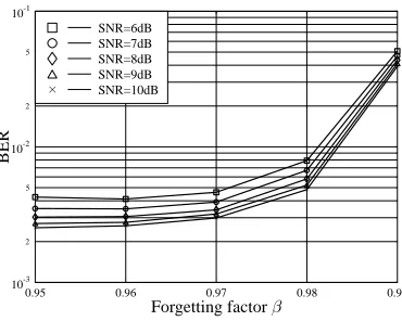
Fig. 3. Mean BER performance against the forgetting factorβin Section IV, when the first two largest eigenvalues are used for uplink transmission at different SNRs. The remaining parameters are the same as in Table II.
-10 -5 0 5 10 SNR (dB)
10-3
2 5
10-2
2 5
10-1
2 5
1
BER
[image:5.595.75.262.328.475.2]Tracked 1st Tracked 2nd Tracked Mean Perfect 1st Perfect 2nd Perfect Mean
Fig. 4. BER versus SNR performance, when the first two eigenvalues are used for uplink transmission. The remaining parameters are the same as in Table II.
In Figure 4 the attainable BER performance is characterized for different values of the SNR, when the first two eigenvalues are used for uplink transmission. The remaining parameters are the same as in Table II. We can see from Figure 4 that the performance recorded for the largest eigenvalue is the same as in Figure 4 and when the availability of perfect channel knowledge is assumed, while the performances achieved by the PATSD algorithm are quite different from theoe seen in Figure 2. This is because the subspace tracking algorithm is unable to eliminate the interferece between the two eigenval-ues, while there is no interference between the two eigenvalues in case of perfect channel knowledge. Furthermore, the BER curve exhibits a floor value upon increasing the SNR. This is because the interference between two eigenvalues becomes the dominant factor for high values of the SNR.
VI. SUMMARY ANDCONCLUSIONS
In this paper, PASTD subspace tracking aided MIMO trans-mit processing techniques were investigated in the context of a TDD system. Since only the left or right singular vectors of the channel matrix are required at transmitter and receiver, respectively, for eigenmode transmission in the TDD mode, PASTD subspace tracking can be used at both the transmitter and receiver to acquire the required left and right singular vectors without estimating the entire MIMO channel matrix
H. This operation is followed by SVD ofH, which typically results in a high complexity. Furthermore, since the PASTD subspace tracking technique is a blind algorithm, it improves the achievable spectral efficiency. A specific deficiency of the family of subspace tracking algorithms is their phase ambiguity imposed by the the non-unique nature of SVD, which was resolved by employing differential encoding. Fi-nally, the efficiency of the proposed scheme was verified by our simulations.
REFERENCES
[1] A. J. Paulraj, D. A. Gore, R. U. Nabar, and H. B¨olcskei, “An overview of MIMO communications - a key to gigabit wireless,” Proceedings of
the IEEE, vol. 92, pp. 198– 218, February 2004.
[2] D. Gesbert, M. Shafi, D. Shiu, P. J. Smith, and A. Naguib, “From theory to practice: an overview of MIMO space-time coded wireless systems,”
IEEE Journal on Selected Areas in Communications, vol. 21, pp. 281–
302, April 2003.
[3] S. N. Diggavi, N. Al-dhahir, A. Stamoulis, and A. R. Calderbank, “Great expectations: the value of spatial diversity in wireless networks,”
Proceedings of the IEEE, vol. 92, pp. 219– 270, February 2004.
[4] S. M. Alamouti, “A simple transmit diversity technique for wireless communications,” IEEE Journal on Selected Areas in Communications, vol. 16, pp. 1451–1458, October 1998.
[5] G. J. Foschini, “Layered space-time architecture for wireless communi-cations in a fading environment using multi-element arrays,” Bell Labs
Technical Journal, vol. 1, pp. 41–59, Autumn 1996.
[6] G. D. Golden, G. J. Foschini, R. A. Valenzuela, and P. W. Wolniansky, “Detection algorithm and initial laboratory results using v-blast space-time communication architecture,” Electronics Letters, vol. 35, pp. 14– 16, January 1999.
[7] I. E. Telatar, “Capacity of multi-antenna Gaussian channels,” European
Transactions on Telecommunications, vol. 10, pp. 585–595, May 1999.
[8] A. S. Dakdouki, V. L. Banket, N. K. Mykhaylov, and A. A. Skopa, “Downlink processing algorithms for multi-antenna wireless commu-nications,” IEEE Communications Magazine, vol. 43, pp. 122 – 127, January 2005.
[9] J. S. Blogh and L. Hanzo, Third-generation systems and intelligent
wireless networking: smart antennas and adaptive modulation. John
Wiley-IEEE Press, 2002.
[10] G. Lebrun, J. Gao, and M. Faulkner, “MIMO transmission over a time-varying channel using SVD,” IEEE Transactions on Wireless
Commu-nications, vol. 4, pp. 757– 764, March 2005.
[11] T. Dahl, N. Christophersen, and D. Gesbert, “Blind MIMO eigenmode transmission based on the algebraic power method,” IEEE Transactions
on Signal Processing, vol. 52, pp. 2424– 2431, September 2004.
[12] A. S. Y. Poon, D. N. C. Tse, and R. W. Brodersen, “An adaptive multi-antenna transceiver for slowly flat fading channels,” IEEE Transactions
on Communications, vol. 51, pp. 1820 – 1827, November 2003.
[13] B. Yang, “Projection approximation subspace tracking,” IEEE
Transac-tions on Wireless CommunicaTransac-tions, vol. 43, pp. 95 – 107, January 1995.
[14] X. Wang and H. V. Poor, “Blind multiuser detection: a subspace approach,” IEEE Transactions on Information Theory, vol. 44, pp. 677– 690, March 1998.
[15] C. Li and X. Wang, “Performance comparisons of MIMO techniques with application to WCDMA systems,” EURASIP Journal on Applied
Signal Processing, vol. 2004, pp. 649–661, May 2004.