White Rose Research Online
[email protected]
Universities of Leeds, Sheffield and York
http://eprints.whiterose.ac.uk/
This is an author produced version of a paper accepted for publication in
Journal
of Nonparametric Statistics.
White Rose Research Online URL for this paper:
http://eprints.whiterose.ac.uk/42950/
Paper
Di Marzio, M and Taylor, CC (2009) Using small bias nonparametric density
estimators for confidence interval estimation. Journal of Nonparametric Statistics,
21 (2). 229 - 240.
Journal of Nonparametric Statistics Vol. 00, No. 00, January 2008, 1–12
RESEARCH ARTICLE
Using small bias nonparametric density estimators for confidence interval estimation
Marco Di Marzioaand Charles C. Taylorb∗
aDMQTE, Universit`a di Chieti-Pescara, Viale Pindaro 42, 65127 Pescara, Italy;bDept.
of Statistics, University of Leeds, Leeds LS2 9JT, UK
(...)
Confidence intervals for densities built on the basis of standard nonparametric theory are doomed to have poor coverage rates due to bias. Studies on coverage improvement exist, but reasonably behaved interval estimators are needed. We explore the use of small bias kernel-based methods to construct confidence intervals, in particular using a geometric density estimator that seems better suited for this purpose.
Keywords:Bootstrap; Coverage rate; Geometric density estimators; Higher-order bias estimators; U-statistic.
AMS Subject Classification: Primary 62G07; secondary 62E20.
1. Introduction
Nonparametric density estimation is plagued by a bias problem, and much effort has been devoted to obtain modified estimators with a smaller bias. [11] perform an extensive, MISE based simulation study where many of these small bias, kernel-based estimators are compared. Their final advice favours the use of the standard kernel method in many situations.
Confidence intervals for nonparametric density estimates typically have poor cov-erage rates as a result of the bias problem. Bootstrap methods do not provide a remedy because the bootstrap expectation of a linear nonparametric estimator is the estimate itself. Hall [5] accurately treats bootstrap confidence intervals for ker-nel density estimation, and concludes that undersmoothing is preferable to explicit bias estimation. After observing that Hall’s undersmoothing deteriorates the vari-ance estimate, and consequently is unable to guarantee the promised coverage, [2] uses empirical likelihood to avoid this reported flaw. To date, it seems that off-the-shelf methods for confidence interval estimation of densities are still needed. In addition, the above studies do not give rules for practical bandwidth selection, and little account is taken of the expected width.
In this paper we explore the feasibility of confidence intervals on the basis of small bias density estimators. Apart from [5], who studies how undersmoothing of higher-order kernel estimators influences the coverage, this strategy has not been fully explored. A reason could be that often many small bias estimators neither
∗Corresponding author. Email: [email protected]
ISSN: 1048-5252 print/ISSN 1029-0311 online c
2008 Taylor & Francis
2 M. Di Marzio & C.C. Taylor
have small theoretical minimum MISEs (as pointed out by [11]), nor possess effi-cient data-driven bandwidth selection. Another reason could be that these methods produce estimates that are not densities. But notice that here the coverage is our main target, therefore the performance of an estimator relies primarily on inte-grated squared bias; much less on MISE. In addition, since our final goal is a confi-dence interval, the fact that the estimate does not integrate to one is of secondary importance. However, the non-negativity constraint – violated by higher-order ker-nel estimators – remains relevant when estimating in the tails.
We focus on a couple of density estimators which implement the same bias re-duction idea, one via a multiplicative structure, and the other one via an addictive structure. Our simulation study compares other known reduced bias estimators for which it is straightforward to obtain a bandwidth selector. Having said that there is an edge for our methods, it seems that all the bias-reduction estimators tried give reasonable performance for confidence interval estimation, even for small samples. In Section 2 we present the estimators. A number of different interpretations are available for them. Unifying views suggest that they rely on the same twic-ing principle or that they have a bootstrap nature. Other different interpretations are possible for the multiplicative version. In Section 3 we obtain asymptotic (inte-grated) mean squared errors. We also formulate normal-based bandwidth selectors, also for a number of estimators included in the paper of [11]. In Section 4 we provide theory to motivate confidence interval estimation, such as asymptotic normality, variance estimation and a Chi-square method to approximate bootstrap distribu-tions. Section 5 contains a simulation study. Finally, some concluding remarks are given in Section 6. A few preliminaries follow.
Given a random sample sample X1, . . . , Xn from an unknown density f of a
continuous r.v. X, the usual kernel density estimate of f at x is
ˆ
f(x;h) := 1
nh
n
X
i=1 K
x−Xi
h
, (1)
the function K, measurable and integrating to 1, is the kernel, the positive real number his the bandwidth. If f has at least p >1 derivatives in a neighbourhood of x, a Taylor series expansion gives
E[ ˆf(x;h)]−f(x) =
p−1 X
k=1
hk(−1)
k
k! f
(k)(x)µ
k(K) +O(hp),
where µk(K) :=
R
ukK(u)du. If K is a density such that µ1(K) = 0 – as in the
standard case – then the bias isO(h2). If an estimator has bias of orderO(hp) with
p >2, we refer to it as a small (or higher-order) bias estimator. K is said to have order p ifµk(K) = 0,0< k < p, and 0< µp(K)<+∞.
2. The estimators
A multiplicative estimator of f at x is
ˆ
fM(x;h) :=
ˆ
f2(x;h) ˆ
it was originally motivated by the observation that the expectation of the smoothed bootstrap normal-kernel estimator is simply ˆf(x; 21/2h). Hence, a standard boot-strap bias correction approach (see [3], pg. 103) leads to the additive estimator
ˆ
fA(x;h) := 2 ˆf(x;h)−fˆ(x; 21/2h)
or the multiplicative estimator ˆfM. ˆfA amounts to (1) equipped with the fourth
order kernel 2K−K∗K, i.e. the “twicing” kernel proposed in fixed design regression by [14]. Although ˆfA is simpler to analyze, we prefer ˆfM because it cannot take
negative values.
The estimator ˆfM is already known, in the sense that [9] cite it as an example
within a family of special cases of a more general technique. This family has been referred to by them as “generalized jackknifing on the log scale”, and ˆfM is thus
an example of a multiplicative form, akin to that of [15]. Although this is a multi-plicative estimator, we note that it is distinct from that of [10]. As it will be seen below, ˆfM has a smaller bias than ˆf, but at the price that it does not integrate
to one. To make the estimator well defined, we require the various denominators to be strictly positive everywhere in the support. This appears a good reason for using Gaussian kernels.
3. Bandwidth selection
The naturalL2risk measure for a generic estimator ˆf(x) isMSE[ ˆf(x)] :=E[{f(x)−
ˆ
f(x)}2]. But, in view of a more general usage, we consider the following global version of it
MISE[ ˆf] :=E
Z
(f −fˆ)2
.
In particular, for a kernel-type estimator ˆf(·;h),h is selected in order to minimize an estimate of an asymptotic version of MISE[ ˆf]. Selectors of this kind are usually indicated as hAMISE. We now give the asymptotic MSEs for our estimators.
Theorem 3.1 : Let X1, ..., Xn be a random sample from a density f of a
contin-uous univariate r.v. X. Given the estimatorsfˆM(x;h) and fˆA(x;h), both equipped
with kernel K, assume that
(1) f is bounded and continuous at x; moreover fiv(x) exists and is finite; (2) the bandwidth h depends on n; in particular limn→∞nh = ∞, and
limn→∞h= 0;
(3) K is a Gaussian density;
Then, at a point x in the support of f we have
E[ ˆfM(x;h)] =f(x) +h
4
4
f′′2(x)
f(x) −f
iv(x)
+O(nh)−1+h6 ,
VAR[ ˆfM(x;h)] =0.72 f(x)
nhπ1/2 +O{(nh)− 2},
MSE[ ˆfM(x;h)] =h
8
16
f′′2(x)
f(x) −f
iv(x)
2
+ 0.72 f(x)
nhπ1/2 +O
4 M. Di Marzio & C.C. Taylor
Table 1. Coefficients ofhAMISE=cˆσn−1/9for various small bias estimators: ˆfMand
ˆ
fAare given in Section 2; ˆfFOis the fourth-order kernel estimator; ˆfJFis an estimator
(explicitly given by (4) in [11]) of [9]; ˆfJLNis that of [10]; ˆfHRis an estimator from
[7], and ˆfTSindicates the variable bandwidth estimator of [16].
Estimator fˆM fˆA fˆFO fˆJF fˆJLN fˆHR fˆTS
c 0.8928 0.9126 1.0834 0.9055 0.9642 0.8617 0.8124
and
E[ ˆfA(x;h)] =f(x) +h
4
4 f
iv(x) +Oh6 ,
VAR[ ˆfA(x;h)] =0.72 f(x)
nhπ1/2 +O{(nh)− 2},
MSE[ ˆfA(x;h)] =h
8
16f
iv(x)2+ 0.72 f(x) nhπ1/2 +O
(nh)−2+h10
Both MSE[ ˆfM(x;h)] and MSE[ ˆfA(x;h)] fit into the general form of MSE expres-sions for small bias estimators in [11].
3.1. Normal Reference Bandwidth Selection
A very simple bandwidth selector for the usual ˆf is thenormal scale rule. It results from a normal population assumption. This gives hNS= 1.06ˆσn−1/5. We now give
similar rules for many small bias estimators. [11] give the approximated AMSE of many O(h4)-bias estimators. All of these, together with the corresponding results for ˆfM and ˆfA, can be integrated under the normal assumption, then optimized
over h. This leads to bandwidth selectors of the form hAMISE = cσnˆ −1/9. The coefficients c are summarized in Table 1.
4. Confidence Interval Estimation
Denote as G an element of{A,M}. To construct a 100(1−α)% confidence interval, we consider normal (IN) and bootstrap percentile (IB) methods:
IN:=
ˆ
fG−zα/2VARˆ [ ˆfG]1/2,fˆG+zα/2VARˆ [ ˆfG]1/2
,
IB:= (FG∗−1(α/2), FG∗−1(1−α/2)),
where FG∗−1(u) := inf{x : F∗
G(x) ≥ u}, with FG∗(x) the bootstrap distribution of
ˆ
fG(x), andVARˆ [ ˆfG] derived below.
The theoretical motivation for using a normal based confidence interval lies in the following
Theorem 4.1 : Given a random sample X1, ..., Xn, taken from a density f of a
continuous univariate r.v. X, then at x in the support of f we have
(nh)1/2{fˆG(x;h)−E[ ˆfG(x;h)]}−→L N
0,0.72f(x) π1/2
if,
• in the case G = M, the assumptions of Theorem 3.1 hold, and, in addition
E[|K(Xi, Xj)|2]<∞ 1≤i, j≤n, where
K(Xi, Xj) :=
1
2{Kh(x−Xi)Kh(x−Xj)−K21/2h(x−Xi) +Kh(x−Xj)Kh(x−Xi)−K21/2h(x−Xj)}.
Finally, if nh5 → 0, the convergence holds true also with f(x) in place of
E[ ˆfG(x;h)].
Proof : See Appendix D.
An alternative to the Normal-based confidence interval, which also avoids the resampling process, follows. By analogy with the estimation of a spectral density [17], approximate FG∗(x) by a scaled χ2 distribution:
Z x
0
a(u)χ2b(u)(u)du
with a(u), b(u) chosen to match the mean and variance of f∗
G(u):
a(x) := VAR∗[fG∗(x)] 2E∗[f∗
G(x)]
, b(x) := 2{E∗[fG∗(x)]}
2
VAR∗[f∗
G(x)] .
whereE∗ andVAR∗are taken with respect to the bootstrap distribution. This leads to a third method denoted as Iχ2.
To obtain an estimator of the variance of ˆfM(x;h), we express it by the expansion in Lemma A of the Appendix – this approximation includes all of the terms of order
O{(nh)−2}, having a residual of orderO{(nh)−3}– then we replacef(x) by ˆf(x;h). We obtain
ˆ
VAR[ ˆfM(x;h)]≃
E[ ˆf2(x;h)]
E[ ˆf(x;21/2h)]
2
VAR[ ˆf2(x;h)]
E[ ˆf2(x;h)]2 +
VAR[ ˆf(x;21/2h)]
E[ ˆf(x;21/2h)]2
−2Ecov[ ˆf2(x;h),fˆ(x;21/2h)] [ ˆf2(x;h)]E[ ˆf(x;21/2h)]
+O{(nh)−3}, (2)
The estimatorVARˆ [ ˆfA(x;h)] is obtainable by similar calculations. In Lemma E the explicit expressions for the estimators involved in the above formula are reported. We notice that VARˆ [ ˆfM(x;h)] is made of ratios with the same bias order both in the numerator and in the denominator. So the bias of VARˆ [ ˆfM(x;h)] is strongly reduced just like the bias of ˆfM(x;h). We note that, in our simulations with small
sample sizes, this estimate of the variance is occasionally negative far in the tails of the distributions. In this case bootstrap intervals can be used.
5. Simulations
6 M. Di Marzio & C.C. Taylor
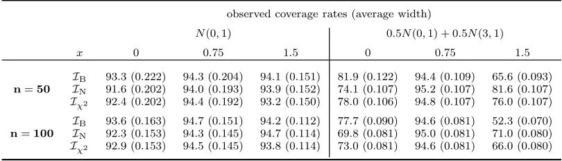
Table 2. Coverages and average widths for various 95% confidence interval estimators atx= 0,0.75,1.5 of a standard normal, and a bimodal density. Methods are: bootstrap percentile; normal approximation; Chi-square approximation. Averages over 100 000 simulations.
observed coverage rates (average width)
N(0,1) 0.5N(0,1) + 0.5N(3,1)
x 0 0.75 1.5 0 0.75 1.5
IB 93.3 (0.222) 94.3 (0.204) 94.1 (0.151) 81.9 (0.122) 94.4 (0.109) 65.6 (0.093)
n=50 IN 91.6 (0.202) 94.0 (0.193) 93.9 (0.152) 74.1 (0.107) 95.2 (0.107) 81.6 (0.107)
Iχ2 92.4 (0.202) 94.4 (0.192) 93.2 (0.150) 78.0 (0.106) 94.8 (0.107) 76.0 (0.107)
IB 93.6 (0.163) 94.7 (0.151) 94.2 (0.112) 77.7 (0.090) 94.6 (0.081) 52.3 (0.070)
n=100 IN 92.3 (0.153) 94.3 (0.145) 94.7 (0.114) 69.8 (0.081) 95.0 (0.081) 71.0 (0.080)
Iχ2 92.9 (0.153) 94.5 (0.145) 93.8 (0.114) 73.0 (0.081) 94.6 (0.081) 66.0 (0.080)
our study. This is in order to check how the performance deteriorates in such scenarios. Curiously, to the best of our knowledge, data driven smoothing is new both for higher order kernels and kernel-based confidence intervals. In particular, higher order estimators have been compared on the basis of their best possible MISEs, while in the only two empirical studies existing on confidence intervals based on kernel density estimators (see [5] and [2]) the coverage rates are reported at predetermined smoothing levels.
In what follows kernels are Gaussian; the bandwidths are given by the normal-based plug-in rules specified in Table 1; the confidence levels are 1−α= 0.95, and, finally, the number of bootstrap samples is 1000.
5.1. Interval estimation
As a first case study, we use the setup of [5]: estimate the standard normal, and a symmetric, bimodal, normal mixture at x= 0,0.75,1.5; use n= 50 and n= 100. Also [2] estimates the standard normal density at 0 with n= 50.
Our results – contained in Table 2 – are averages over 100 000 simulations. It can seen that our coverage favorably compares with those of [5] and [2]. In particular,
IN works also for these small sized samples, yet its theoretical motivation has an
asymptotic nature. It is noticeable that Iχ2 also performs well. For the bimodal
density, the coverage at x= 1.5, which is a local minimum, is, as expected, poor. But it is still superior to most of the performances seen in [5].
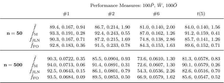
The second case study is more general: we estimate models #1 (Gaussian), #2 (Skewed Unimodal) and #6 (Bimodal) of [12] in [−3,3]; moreover a Studenttwith five degrees of freedom in [−4,4]. Sample sizes are 50 and 500. As a motivation for this choice consider that we have included the main three unimodal models, i.e. symmetric, skewed and heavy tailed, to obtain a more general conclusion on the matter. We compute bootstrap percentile confidence intervals based on various es-timators. Concerning our choice of estimators, consider what follows. It is possible to divide small bias methods into two categories, depending on their output: “pos-itive” estimators and “negative” ones. Now, from the extensive comparative study provided by [11], it results that excellent candidates to represent these categories are, respectively, the proposal of [10] ( ˆfJLN), and the fourth-order kernel estimator in Section 2.1 of [11] ( ˆfFO). As a benchmark, also ˆf is included.
We adopt the following performance indices:
P :=
Z
Table 3. Integrated performance measures ¯P ,W ,¯ O¯ (10 000 simulations) for a variety of bootstrap 95% percentile confidence intervals (indicated by the corresponding point estimator symbol).
Performance Measures: 100 ¯P, ¯W, 100 ¯O
#1 #2 #6 t(5)
ˆ
f 89.4, 0.167, 0.94 86.7, 0.214, 1.90 81.0, 0.140, 2.00 84.0, 0.140, 1.56
n=50 fˆM 93.3, 0.191, 0.28 92.4, 0.243, 0.55 87.0, 0.162, 1.26 91.2, 0.159, 0.41
ˆ
fJLN 90.3, 0.167, 0.71 87.2, 0.215, 1.69 74.8, 0.138, 2.86 85.7, 0.141, 1.26
ˆ
fFO 92.8, 0.183, 0.36 91.5, 0.233, 0.78 84.3, 0.153, 1.63 89.6, 0.152, 0.71
ˆ
f 90.3, 0.0722, 0.35 85.5, 0.0904, 0.93 73.6, 0.0610, 1.30 81.3, 0.0578, 0.83
n=500 fˆM 94.0, 0.0713, 0.06 91.4, 0.0891, 0.31 72.6, 0.0607, 1.30 90.1, 0.0579, 0.26
ˆ
fJLN 92.5, 0.0643, 0.15 86.1, 0.0801, 0.79 54.3, 0.0536, 2.26 82.6, 0.0516, 0.70
ˆ
fFO 93.5, 0.0684, 0.09 89.5, 0.0853, 0.50 66.9, 0.0579, 1.62 85.6, 0.0547, 0.52
W :=
Z
w(x)f(x)dx,
the expectations of the coverage (p) and width (w). Strictly, narrower intervals are of importance only when the desired coverage is attained, so the trade-off we have used is
O :=
Z
|1−α−p(x)|w(x)f(x)dx .
Table 3 gives the results for each of the measures P, W, O calculated on 10 000 samples. It can be seen from Table 3 that small bias methods give much better coverage than ˆf, recalling that the bandwidth is always automatically selected. The results for ˆfA (not shown) were quite similar to those of ˆfM, but not quite as
good. Overall, it seems that ˆfM is well behaved for the unimodal case. In order to
investigate why ˆfM seems to outperform ˆfJLN and ˆfFO, we now consider a more
typical analysis of performance in point estimation.
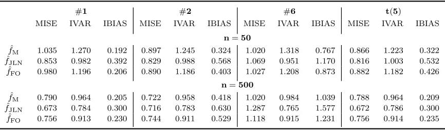
5.2. Point estimation
For the same models and estimators as before, we have calculated the usual L2
integrated discrepancies. For each model 10 000 samples were drawn. Each column of Table 4 gives the ratio of MISE, integrated variance and integrated bias-squared between an element of {fM,ˆ fJLN,ˆ fFOˆ } and those of ˆf. As can be seen from Table 4, ˆfM is the best in bias reduction, even though it is not so good at minimizing
MISE. Now, note that in presence of bias (small bias estimators are still biased) we will need the variance to have a bigger magnitude than bias, in order to get the right coverage. But this is exactly the case of ˆfM, on the basis of Table 4, where we
can observe comparatively small biases and big variances. In conclusion, the point estimation results, if read from a confidence interval perspective, explain a certain superiority of ˆfM.
5.3. On normalizing the estimators
8 M. Di Marzio & C.C. Taylor
Table 4. Integrated performance measures for a variety of estimators and models. Ratios of estimators (fe∈ {fˆM,fˆJLN,fˆFO}),
for MISE, integrated variance, and integrated bias-squared, relative to those of ˆf, i.e.MISE[fe]/MISE[ ˆf],IVAR[fe]/IVAR[ ˆf], and IBIAS[fe]/IBIAS[ ˆf]. Quantities are averages over 10 000 simulations.
#1 #2 #6 t(5)
MISE IVAR IBIAS MISE IVAR IBIAS MISE IVAR IBIAS MISE IVAR IBIAS
n=50
ˆ
fM 1.035 1.270 0.192 0.897 1.245 0.324 1.020 1.318 0.767 0.866 1.223 0.322
ˆ
fJLN 0.853 0.982 0.392 0.829 0.988 0.568 1.069 0.951 1.170 0.816 1.003 0.532
ˆ
fFO 0.980 1.196 0.206 0.890 1.186 0.403 1.027 1.208 0.873 0.882 1.182 0.426
n=500
ˆ
fM 0.790 0.964 0.205 0.722 0.958 0.418 1.020 0.984 1.039 0.788 0.964 0.209
ˆ
fJLN 0.673 0.784 0.300 0.716 0.783 0.630 1.287 0.765 1.577 0.672 0.786 0.300
ˆ
fFO 0.756 0.913 0.230 0.744 0.911 0.529 1.118 0.915 1.231 0.756 0.914 0.235
performance of an estimator — both absolute and relative — to a subjective choice of the correction method. It would be a subjective choice exactly because the for-mal properties of these estimators refer to the uncorrected versions. The only fair alternative could have been to select the best correction method for each pair
{estimator, model}, but this seems a long way from practical usage. However, we note that the correction subject seems problematic, for example, [4] show that the simple dividing by the integral of the estimate – inappropriate for correcting higher-order kernel methods – could even deteriorate the performance, depending on the model to estimate, and with no way to know this in advance from the data.
6. Concluding Remarks
Higher-order bias methods have been much studied in kernel density estimation, but are less used. Given that, in some cases, explicit bias correction of an ordinary kernel is essentially equivalent to using a small bias estimator [8], there seems to be justification for using such methods when the goal is confidence interval estimation rather than point estimation. In this case, it seems that the strength of any method lies mainly in its ability to reduce bias with the availability of a suitable plug-in rule for the smoothing parameter. Further work could extend these methods to nonparametric regression, which could also be incorporated in hypothesis testing, for example, in tools such as SiZer [1].
Finally, we note that our data-based smoothing parameters are chosen to min-imize AMISE (under a normal assumption). However (as also pointed out by [5]) there is absolutely no reason that an adequate choice for the bandwith which min-imizes MISE will be the correct one in terms of coverage accuracy. However, our simulations suggest that these AMISE-bandwidth selectors may nevertheless pro-vide a good trade-off between coverage and expected width in many situations. Moreover, practical selectors which “optimize” the coverage do not yet exist.
Acknowledgements
References
[1] P. Chaudhuri and J.S. Marron,SiZer for exploration of structures in curves, J. Amer. Statist. Assoc. 94 (1999), pp. 807–823.
[2] S.X. Chen,Empirical likelihood confidence intervals for nonparametric density estimation, Biometrika 83 (1996), pp. 329–341.
[3] A.C. Davison and D.V. Hinkley,Bootstrap Methods and Their Application, Cambridge: Cambridge University Press, 1997.
[4] I.K. Glad, N.L. Hjort, and N. Ushakov,Correction of density estimators that are not densities, Scand. J. Statist. 30 (2003), pp. 415–427.
[5] P. Hall,Effect of bias estimation on coverage accuracy of bootstrap confidence intervals for a proba-bility density, Ann. Statist. 20 (1992), pp. 675–694.
[6] W. Hoeffding,A class of statistics with asymptotically normal distribution, Ann. Math. Statist. 19 (1948), pp. 293–325.
[7] O. H¨ossjer and D. Ruppert,Asymptotics for the transformation kernel density estimator, Ann. Statist. 23 (1995), pp. 1198–1222.
[8] M.C. Jones,On higher order kernels, J. Nonparametr. Stat. 5 (1995), pp. 215–221.
[9] M.C. Jones and P.J. Foster,Generalized Jackknifing and higher order kernels, J. Nonparametr. Stat. 3 (1993), pp. 81–94.
[10] M.C. Jones, O. Linton and J.P. Nielsen, A simple bias reduction method for density estimation, Biometrika 82 (1995), pp. 327–38.
[11] M.C. Jones and D.F. Signorini,A comparison of higher-order bias kernel density estimators, J. Amer. Statist. Assoc. 92 (1997), pp. 1063–1073.
[12] J.S. Marron and M.P. Wand,Exact mean integrated squared error, Ann. Statist. 20 (1992), pp. 712– 736.
[13] R.J. Serfling,Approximation Theorems of Mathematical Statistics, Wiley, New York, 1980.
[14] W. Stuetzle and Y. Mittal,Some comments on the asymptotic behavior of robust smoothers, inLecture Notes in Math 757: Smoothing Techniques for Curve Estimation, T. Gasser and M. Rosemblatt, eds., Springer-Verlag, Berlin, 1979, pp. 191-195.
[15] G.R. Terrell and D.W. Scott,On improving convergence rates for nonnegative kernel density estima-tors, Ann. Statist. 8 (1980), pp. 1160–1163.
[16] G.R. Terrell and D.W. Scott,Variable kernel density estimation, Ann. Statist. 20 (1992), pp. 1236– 1265.
[17] J.W. Tukey, The sampling theory of power spectrum estimates inProc. Symp. on Applications of Autocorrelation Analysis to Physical Problems, NAVEXOS–P-735, Office of Naval Research, Depart-ment of the Navy, Washington, USA, 1949, pp. 47–67.
Appendix A. Lemma A
Consider two continuous, real random variables X and Y, If bothµX and µY are
non-zero, and VAR[X/Y] exists finite, then
VAR
X Y
≃
µX
µY
2σ2
X
µ2
X
+σ
2
Y
µ2
Y
− 2σXY µXµY
,
provided that all the involved moments are finite.
Proof : This standard result is obtained by calculating the expectation of the second-order bivariate Taylor expansion ofX/Y in a neighborhood of (µX, µY).
Appendix B. Lemma B
Consider a random sample X1, ..., Xn, taken from a continuous univariate density
f. Let φ(h) := E[Kh(x−X1)] where x belongs to the support of f. Assume that the kernel K is a Gaussian density. Then
E[ ˆf2(x;h)] = 1
n
(n−1)φ(h)2+φ(h/2
1/2)
2π1/2h
,
10 REFERENCES
VAR[ ˆf(x; 21/2h)] = 1
n
φ(h)
81/2π1/2h −φ(2 1/2h)2
,
n4VAR[ ˆf2(x;h)] =n
φ(h/2) 321/2π3/2h
3/2− φ(h/21/2)2
4πh2
+ 2n! (n−2)!
φ(h/21/2)2
4πh2 −φ(h) 4
+ 4n! (n−3)!
φ(h)2
φ(h/21/2)
2π1/2h −φ(h) 2
+ φ(h)
n−3
φ(h/31/2)
121/2πh2 −
φ(h/21/2)
2π1/2h φ(h)
,
COV[ ˆf2(x;h),fˆ(x; 21/2h)] = n! (n−2)!
(n−2)φ(h)2φ(21/2h) + φ(h/2
1/2)
2π1/2h φ(2 1/2h)
+2φ((2/3)
1/2h)
61/2π1/2h φ(h)
+ n
201/2πh2φ((2/5)
1/2h)− 1 n
(n−1)φ(h)2+ φ(h/2
1/2)
2π1/2h
.
Proof : The first three equations are immediate. SetYi:=x−Xi, now
VAR[fb2(x;h)] = 1
n4VAR
hX X
Kh(Yi)Kh(Yj)
i ,
then n4VAR[fb2(x;h)] is equal to
nVARKh(Y1)2+ 2 n!
(n−2)!VAR[Kh(Y1)Kh(Y2)] +
n!
(n−4)!COV[Kh(Y1)Kh(Y2), Kh(Y3)Kh(Y4)]
+4 n!
(n−3)!COV[Kh(Y1)Kh(Y2), Kh(Y1)Kh(Y3)] + 2
n!
(n−3)!COV[Kh(Y1)Kh(Y1), Kh(Y2)Kh(Y3)]
+4 n!
(n−2)!COV[Kh(Y1)Kh(Y1), Kh(Y1)Kh(Y2)] +
n!
(n−2)!COV[Kh(Y1)Kh(Y1), Kh(Y2)Kh(Y2)].
Assuming that the kernel is Gaussian, a little algebra leads to the result. Concerning the mixed moment of COV[ ˆf2(x;h),fˆ(x; 21/2h)], we have
n3X X XE[Kh(Yi)Kh(Yj)K21/2h(Ys)] =
n!E[Kh(Y1)Kh(Y2)K21/2h(Y3)]
(n−3)!
+n!E[Kh(Y1)
2K
21/2h(Y2)]
(n−2)! + 2
n!E[Kh(Y1)Kh(Y2)K
21/2h(Y1)]
(n−2)! +nE[Kh(Y1)
2K
21/2h(Y1)].
Assuming that the kernel is Gaussian, again a little algebra leads to the result.
Appendix C. Proof of Theorem 3.1
The proof is based on a “linearization” argument. First of all, we note that
{fˆM(x;h)−f(x)} −
(
ˆ
fh(x;h)2−f(x) ˆf(x; 21/2h)
f(x)
) ∼op
n
and so the bias is approximated by the expectation of the second term, i.e.
E[ ˆf(x;h)2]−f(x)E[ ˆf(x; 21/2h)]
f(x) =
h4
4
f′′(x)2
f(x) −f
iv(x)
+O(h6) +O(nh)−1 .
Now let fn(x) :=E[ ˆf(x;h)2]/E[ ˆf(x; 21/2h)] and note that
ˆ
fM(x;h)−fn(x) =
"
ˆ
f(x;h)2
f(x) − ˆ
f(x; 21/2h)fn(x)
f(x)
#
f(x) ˆ
f(x; 21/2h).
Since
f(x) ˆ
f(x; 21/2h)
p
−→1
the variance of the LHS is equal to the variance of the term in square brack-ets. Lemma B provides the various elements. For an approximate version of VAR[ ˆfM(x)], consider that ¯φ(h) =f(x) +h2f′′(x)µ2(K) +O(h4) and replace ¯φ(h) with f(x). Finally consider that K is a Gaussian density. To get the asymptotic moments of ˆfA(x;h) apply Lemma B, then approximate as above.
Appendix D. Proof of Theorem 4.1
We have
ˆ
fA(x;h) =
1
nh
n
X
i=1 H
x−Xi
h
where H(z) := 2K(z)−1/21/2K(z/21/2), a higher order kernel. But the Lindberg condition holds, as for the standard kernel, as follows. For any ǫ >0,
h−1E
" H
x−X1
h 2
I{|H(x−X1 h )−E[H(
x−X1 h )]|>
√
nhǫ} #
=
Z
{|H(y)−E[H(x−X1 h )]|>
√
nhǫ}H(y)
2f(t−hy)dy
which converges to 0 if nh→ ∞.
Concerning ˆfM, as seen in the proof of Theorem 3.1, ˆfM(x;h) − fn(x) and
ˆ
f(x;h)2/f(x)−fˆ(x; 21/2h)f
n(x)/f(x) have the same asymptotic distribution. So
it is sufficient to prove that
n1/2{Vn−E[Vn]}−→L N(0,4ζ1)
with Vn:= ˆf(x;h)2−fˆ(x; 21/2h) and ζ1:=VAR[R K(X1, x2)f(x2)dx2]>0.
We have
Vn=
1
n2
X X
1≤i,j≤n
12 REFERENCES
Now observe thatK(Xi, Xj) =K(Xj, Xi) 1≤i, j≤n, thereforeVn is a von Mises
statistic. Now define the U-statistic Vn∗ := {n(n−1)}−1P P1≤i6=j≤nK(Xi, Xj).
Provided thatE[|K(Xi, Xj)|2]<∞ 1≤i, j≤n,we haven1/2(Vn−V∗
n) p
−→0 (see [13], pg. 206). Now,
n1/2{Vn∗−E[V∗
n]} L
−→N(0,4ζ1)
provided thatVAR[Ke(X1)]>0,whereKe(x1) :=E[K(x1, X2)] (see [6]). But observe that
E[K(x1, X2)] =Kh(x1−x)E[Kh(X2−x)]−1
2{K21/2h(x1−x) +E[K21/2h(X2−x)]},
which is not degenerate. Finally, if nh5→0,
lim
n→∞{
E[ ˆfG(x;h)]−f(x)}= lim
n→∞(nh)
1/2O(h4) = 0.
Appendix E. Lemma E
The expressions of the estimators contained in formula (2) are listed below
ˆ
E[ ˆf2(x;h)] = (n−1) ˆf
2(x; 21/2h) + ˆf(x; (3/2)1/2h)/(2π1/2h)
n2 ;
ˆ
E[ ˆf(x; 21/2h)}= ˆf(x; 31/2h) ;
ˆ
VAR[ ˆf(x; 21/2h)] = 1
n ˆ
f(x; 21/2h) 81/2π1/2h −fˆ
2(x; 31/2h)
;
n3VARˆ [ ˆf2(x)] = 4(n−1)(n−2) ˆf2(x; 21/2h)
ˆ
f(x; (3/2)1/2h)
2π1/2h −fˆ
2(x; 21/2h)
+
ˆ
f(x; (5/4)1/2h) 321/2π3/2h3 −
ˆ
f2(x; (3/2)1/2h) 4πh2
+ 2(n−1)
ˆ
f2(x; (3/2)1/2h)
4πh2 −fˆ
4(x; 21/2h)
+4(n−1) ˆf(x; 21/2h)
ˆ
f(x; (4/3)1/2h) 121/2πh2 −
ˆ
f(x; 21/2h) ˆf(x; (3/2)1/2h) 2π1/2h
;
n2COVˆ
h
ˆ
f2(x;h),fˆ(x; 21/2h)i= 2(n−1) 61/2π1/2hfˆ(x; 2
1/2h) ˆf(x; (5/3)1/2h)
−fˆ(x; (3/2)
1/2h) ˆf(x; 31/2h)
2π1/2h −2(n−1) ˆf
2(x; 21/2h) ˆf(x; 31/2h) + fˆ(x; (7/5)1/2h)
![Table 1.Coefficients of hAMISE = cσnˆ−1/9 for various small bias estimators: fˆM andfˆA are given in Section 2; ˆfFO is the fourth-order kernel estimator; ˆfJF is an estimator(explicitly given by (4) in [11]) of [9]; fˆJLN is that of [10]; fˆHR is an estimator from[7], and fˆTS indicates the variable bandwidth estimator of [16].](https://thumb-us.123doks.com/thumbv2/123dok_us/8006827.210556/5.595.105.441.80.252/coecients-estimators-estimator-explicitly-estimator-indicates-bandwidth-estimator.webp)