Rochester Institute of Technology
RIT Scholar Works
Theses
8-16-2018
Robust Path-based Image Segmentation Using
Superpixel Denoising
Renee T. Meinhold
Follow this and additional works at:
https://scholarworks.rit.edu/theses
This Thesis is brought to you for free and open access by RIT Scholar Works. It has been accepted for inclusion in Theses by an authorized administrator of RIT Scholar Works. For more information, please [email protected].
Recommended Citation
Robust Path-based Image
Segmentation Using Superpixel
Denoising
by
R
enee
T. M
einhold
A Thesis Submitted in Partial Fulfillment of the Requirements
for the Degree of Master of Science in Applied and Computational Mathematics
School of Mathematical Sciences, College of Science
Rochester Institute of Technology
Rochester, NY
Committee Approval:
Dr. Nathan Cahill
School of Mathematical Sciences
Thesis Advisor
Date
Dr. Nathaniel Barlow
School of Mathematical Sciences
Committee Member
Date
Dr. Kara Maki
School of Mathematical Sciences
Committee Member
Date
Dr. John Hamilton
School of Mathematical Sciences
Committee Member
Date
Dr. Matthew Hoffman
School of Mathematical Sciences
Director of Graduate Programs
Abstract
C
ontents
I Introduction 1
II Introduction to Clustering and Image Segmentation 4
II.1 Centroid-based clustering . . . 4
II.2 Hierarchical clustering . . . 5
II.3 Graph-based spectral clustering . . . 7
II.4 Image segmentation . . . 9
II.4.1 Defining the Weight Matrix for Graph-based Image Segmentation . . . 9
II.4.2 Image Segmentation Algorithms . . . 11
II.4.3 Superpixel Representation . . . 13
III Longest-Leg Path Distance Ultrametric 16 III.1 Definition . . . 16
III.2 Prior research . . . 17
III.3 Computation . . . 18
III.4 Advantages and disadvantages for use in spectral clustering . . . 20
IV Path-based Clustering Denoising by Pre-cluster Averaging 23 IV.1 Motivation . . . 23
IV.2 Out-of-sample extension of a Laplacian-Eigenmaps embedding . . . 26
IV.3 Spatial-smoothing techniques for out-of-sample image segmentation . . . 27
IV.4 General algorithm for image segmentation . . . 28
IV.5 Linear interpolation of superpixel embedding . . . 30
V Image Experiments and Results 32 V.1 LLPD in images . . . 32
V.2 Segmentation evaluation criteria . . . 33
V.3 Image segmentation experiments . . . 35
V.4 Results . . . 36
V.5 Varying of parameters for interpolation segmentation . . . 38
VI Conclusion and Future Directions 40 VI.1 Conclusion . . . 40
VI.2.1 More sophisticated methods of smoothing final embedding . . . 41
VI.2.2 Application to hyperspectral images for target detection . . . 42
VI.2.3 Computational improvement . . . 42
VI.2.4 Impact of the Bandwidth Parameter . . . 42
L
ist of
F
igures
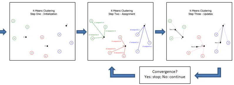
1 Outline of k-means iteration scheme. This process is initialized by assigning k
random central vectors shown in Step One, then each point is then assigned to
its closest central vector in Step Two. Thekcentral vectors are then recomputed
as the average of all points assigned to it, and Steps Two and Three are repeated
until the central vectors have converged to a point within a user specified tolerance.
Visualizations from http://www.turingfinance.com . . . 5
2 (a) Two-dimensional data set with four high density clusters surrounded by low
density noise, (b) Corresponding single linkage dendrogram for data set of (a).
Figure from [1]. . . 6
3 Example of segmented image. (a) Original image, (b)k=2, (c)k=5, (d)k=10. . . 9
4 Examples of superpixel calculation using SLIC algorithm. By columns, Left: Original
image, Middle left: Outlines of region size 10 superpixels, Middle: Region Size 10
superpixels displayed with average color and mean position as black dot, Middle
right: Outlines of region size 20 superpixels, Right: Region Size 20 superpixels
displayed with average color and mean position as black dot. . . 14
5 Normalized cut image segmentations using superpixels for k=5, with each pixel
being assigned the label of its superpixel. . . 15
6 (a) Four Lines Data Set, (b) Plot of each point’s K=10th LLPD nearest neighbor
in ascending order, points withKthLLPD nearest neighbor distance above the red
line are considered noise and removed, (c) Plot of data with noise as red circles and
cluster data as blue circles, (d) L2 clustering results, (e) LLPD clustering results, (f)
40 smallest eigenvalues for L2 and LLPD embedding. . . 20
7 (a) LLPD clustering results without denoising, (b) 40 smallest eigenvalues for LLPD
embedding without denoising. . . 21
8 Comparison of L2 to LLPD from the point p= (1.1910, 0.2114)in an artifical data
set with and without noise. (a) L2 distances from pwithout noise, (b) LLPD from p
without noise, (c) L2 distances from pwith 10 added data points of noise, (d) LLPD
distances from pwith 10 added data points of noise. . . 22
9 Clustering by preclustering on three artificial data sets: Four Lines (Row 1), Nine
Gaussians (Row 2), and Three Arcs (Row 3). Columns left to right: Original data set,
pre-clustering reduced data set, LLPD clustering of reduced data, corresponding
10 (a) Original Image, (b) LLPD segmentation of full image without noise reduction
for k=4 segments, with the background class represented by average color and
three noise classes represented by red, green, and blue for clarity (c) Superpixel
visualization of approximately 6×6 pixels each, (d) LLPD segmentation using
superpixels of (c) for k = 4 segments. Using superpixels allows for the main
structure of the image to be visible after segmentation whereas segmentation of the
full image identifies noisy pixels as clusters. . . 25
11 Flowchart of superpixel denoising with extension method. . . 29
12 Normalized cut image segmentations using superpixels fork=5. First row: original
image, Second row: each pixel is assigned the label of its superpixel, Third Row:
Interpolating of the superpixel embedding over the spatial coordinates of the image. 31
13 (a) Original Image, (b) Color representation of LLPD pixel degree, (c) Color
repre-sentation of LLPD pixel degree , (d) Contours of image given by sharp changes in
LLPD pixel degree . . . 32
14 L2- (top row) and LLP- (bottom row) distances to all superpixels from chosen
superpixel outlined in red. By column left to right, the chosen superpixel is located
on the body of the bird, the black colored facial area, the lower branches, and the
upper background. . . 33
15 Segmentations for images in the BSDS-500 data set, by column from left to right:
Original Image, L2 interpolation, LLPD interpolation, LLPD out-of-sample
exten-sion, LLPD sample extension with post-spatial smoothing, LLPD
out-of-sample extension with pre-spatial smoothing . . . 37
16 Segmentations with varying α values fork = 10, with the first row showing L2
segmentations and the second row showing LLPD segmentations. By column, (a)
Original image, (b)α=0, (c)α=0.2, (d)α=0.4, (e)α=0, 6, (f)α=0.8, (g)α=1. 39
17 Segmentations with varying kvalues forα = 0.5, with the first row showing L2
segmentations and the second row showing LLPD segmentations. By column, (a)
L
ist of
T
ables
I.
I
ntroduction
Clustering, the process of partitioning a data set into groups with similar characteristics, is an
important automated task with uses in many fields. Many techniques have been created to solve
this problem, with one of the most popular being spectral clustering [2]. A spectral clustering
method represents the data as a graph where vertices represent data points and edges show the
similarity between those data points, and then computes a new representation, or embedding, of
each data point based on the eigendecomposition of an affinity matrix representing graph edges.
The populark-means clustering algorithm can then be applied to the embedded coordinates to
compute the final point labels. Althoughk-means is limited in capability for data on a manifold in
a high-dimensional space, the embedding produced by the spectral clustering procedure gives a
basis for a lower-dimensional representation that preserves local relationships, allowing for this
simpler clustering procedure to perform well in the embedding space.
An important component of spectral clustering methods is how the affinity matrix is defined. A
common method employs a Gaussian kernel using the Euclidean distance between data points;
however, this often performs poorly for elongated or non-convex clusters where data points
may be separated by a large Euclidean distance but are connected by a high density of points.
Therefore, for data sets composed of high density clusters with low density noise, a path-based
distance metric between points can overcome these challenges. The longest-leg path distance
(LLPD) between vertices on a graph is the minimum edge weight such that all unique paths
between the two vertices contain an edge of at least this weight, and has been shown to perform
well in spectral clustering, where edges are weighted by Euclidean distance to compute the LLPD,
under certain assumptions about the data model [1]. The LLPD, however, is sensitive to noise
and outlying data points, so denoising before computing an LLPD spectral clustering is necessary.
Denoising schemes usually rely on identifying and removing noise points before computing the
spectral clustering.
The removal of outlying points from a data set may be difficult or unreasonable for certain data
sets, like images, that have a specific structure. The clustering problem applied to images is known
as image segmentation, and it involves partitioning an image into regions containing similar pixels,
where similarity is based on both spatial and feature components. Removing image pixels from an
image data set thus interrupts the spatial continuity of the final segmentation as well as the spatial
similarity between two image pixels. However, keeping allN Mpixels of anN×Mimage can be
eigenvectors of anN M×N Mmatrix, and even an average sized image can contain hundreds of thousands of pixels.
In this thesis, we propose a new method for robustly performing LLPD spectral clustering. This
method first denoises the data set by performing a pre-clustering of the data on a fine scale,
meaning the number of pre-clusters is much larger than the final number of data clusters desired,
but much less than the total number of data points. All data points in a pre-cluster are then
averaged to form a reduced data set. Under the assumption that noise points are of a much lower
density than cluster points, a large enough pre-cluster will contain mostly cluster data points with
only a few noise points. Averaging all point in a pre-cluster will largely reflect the relevant cluster
data, making the effect of noise much smaller. The spectral clustering algorithm is applied to the
reduced data set, yielding an embedding of the reduced data set that is robust to noise of the full
data set. The embedding is extended back to the full data set using an out-of-sample extension
technique [26] to get the final clustering.
For an image, pre-clusters can be computed by oversegmenting an image into a few hundred
or thousand small spatial regions of similar pixels called superpixels [16]. These superpixels
are then represented by the mean color or feature and spatial location of all component pixels
and an embedding is computed based on a graph whose vertices are defined over the set of
superpixels. Since image pixels are defined at a known spatial locations, the embedding can be
extended to each pixel location by a simple spatial interpolation, as opposed to the more general
out-of-sample extension technique. The spatial interpolation method is much less computationally
expensive for LLPD spectral clustering, but it lacks the mathematical foundation of the
out-of-sample extension. Both methods have the advantage over other techniques that the noise does
not have to be identified specifically, and significantly reduces the size of the eigendecomposition
problem.
The goal of this thesis is to enable robust image segmentation via approximate LLPD spectral
clustering, and show the advantage of this method employing path-based distances over the use
of the standard euclidean distance. This thesis is organized as follows: Section 2 provides an
introduction to several clustering techniques pertinent to this research and an introduction to
basic concepts of image segmentation. Section 3 explains various aspects of the LLPD including
its formal definition, prior uses in clustering, computation, and specific advantages. Section 4
introduces our new denoising method providing specific motivating examples, mathematical
background, schematic for computing, and optional spatial smoothing. We also discuss the simpler
image segmentation tests on the publicly available BSDS-500 [21] data set in Section 5, comparing
L2 and LLPD spectral clustering, and comparing out-of-sample extension to spatial interpolation
methods. The results are discussed both qualitatively and quantitatively in the context of well
known segmentation performance measures [14]. Section 6 concludes the thesis by summarizing
II.
I
ntroduction to
C
lustering and
I
mage
S
egmentation
Given a set of data pointsX={x1,x2, . . . ,xn}withxi ∈Rm, the process of partitioningXinto
a set of k groups with similar characteristics C = {C1,C2, . . . ,Ck} is calledclustering, withC
often referred to asa clustering of X. We assume for this thesis thatCis a strict partitioning ofX,
meaning it is exhaustive and all clusters are mutually exclusive, however there is a separate body
of work known as "fuzzy" clustering allowing each data point to belong to more than one cluster.
Clustering is an unsupervised learning technique, which, unlike supervised learning techniques,
assumes that there are no response variablesY={y1,y2, . . . ,yn}corresponding to each data point.
This is one of the most fundamental problems of machine learning because of its applicability
to problems in a wide variety of fields, such as pattern recognition, bioinformatics, finance, and
image processing. As such, many different approaches have been proposed to solve this problem.
The subgroups of solution techniques that are most relevant to this research are centroid-based,
hierarchical, and graph-based clustering, each of which are summarized below.
II.1
Centroid-based clustering
Centroid-based clustering represents each clusterCjwith a central vector ˆCj, then createskclusters
by minimizing the sum of the squared Euclidean distances between ˆCjand each data pointx∈Cj.
The most popular centroid-based clustering algorithm is thek-means algorithm where the central
vector is the average of the data points in its cluster,
ˆ
Cj=x¯j = 1
|Cj| x
∑
∈Cjx. (II.1)
The optimization problem of thek-means algorithm can then be written formally as
C∗=arg min
C
k
∑
j=1x
∑
∈Cjkx−x¯jk22, (II.2)
whereC∗is thek−means clustering. Finding the exact solution of Equation II.2 is NP-hard, but
the solution can be easily and quickly approximated with an iteration scheme, initialized byk
random points inRmrepresenting thekcluster vectors. Each data point is then assigned to the
process is then repeated until the central vectors converge. An outline of this process is displayed
[image:14.612.111.509.139.285.2]in Figure 1.
Figure 1:Outline ofk-means iteration scheme. This process is initialized by assigningkrandom central vectors shown in Step One, then each point is then assigned to its closest
central vector in Step Two. Thekcentral vectors are then recomputed as the average
of all points assigned to it, and Steps Two and Three are repeated until the central
vectors have converged to a point within a user specified tolerance. Visualizations from
http://www.turingfinance.com
This approximate solution, however, can be dependent on initialization since the iteration scheme
may converge to a local minimum. Therefore, computing the clustering for different initializations
may be necessary. A limitation of k-means clustering is that it has been shown to perform
inadequately for data sets composed of poorly separated, noisy, and/or non-spherical clusters.
Because of these limitations, a variety of more sophisticated techniques (including spectral
clustering) first compute or define a new representation of the data in which these problems are
lessened, followed by k-means clustering on the new representation.
II.2
Hierarchical clustering
Hierarchical clustering methods form a set ofnnested clusterings of a data setX, each containing
a different number of clusterskranging from 1 ton. These techniques can be categorized as either
agglomerative or divisive. An agglormerative method initially considers each data point as a
cluster and iteratively merges the two most similar clusters, while a divisive algorithm initially
dissimilarity.
Deciding which regions to merge or break defines specific hierarchical clustering methods. This is
done by defining a distance between pairs (potential pairs) of clusters, and choosing the clusters
with the minimum (maximum) of those distances to merge (break). Most technical research
has been focused on agglomerative methods, of which complete linkage, group average, and
single linkage are some of the most well known. Complete linkage clustering defines the distance
between two clusters as the maximum distance of the distances between two points drawn from
separate clusters. Group average clustering takes the average distance of all inter-cluster data
pairs as the cluster distance. Single linkage clustering defines cluster distance as the minimum
distance of all inter-cluster data pairs. Single linkage clustering tends to produce a "chaining"
effect, causing unbalanced clusters by retaining single outlying data points as clusters until the
final iterations [6].
All these cluster distances obey the utlrametric property, which guarantees that once two clusters
are merged or a cluster is broken, they cannot be separated or merged again in future iterations.
The ultrametric property will be discussed in the next section in detail. This allows for the
creation of a hierarchical structure that can be represented by a dendrogram, of which the height
represents the value at which each cluster merge or break is made. An example of a data set and
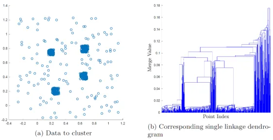
its corresponding single linkage dendrogram is shown in Figure 2. It is then up to the user to
decide at which height to retrieve a clustering, defining how many clusters are appropriate. This
is not always obvious however, especially with noisy data. For example, it is not readily seen from
[image:15.612.168.449.489.633.2]the dendrogram of Figure 2 that the data set is composed of four clusters.
Figure 2:(a) Two-dimensional data set with four high density clusters surrounded by low density
II.3
Graph-based spectral clustering
Graph-based clustering relies on representing the data setXas a weighted undirected graph with
vertices representing the data points and weighted edges the similarity between the data points.
Edges with high weight signify that the two connected data points are very similar and should
likely be placed in the same group. Dissimilar data points are connected by edges with low or
zero weight, and likely should be placed in different groups.
Formally, let G = (V,E) be an undirected graph consisting of the set of verticesV = X and
edgesE. To specify the weight of each edge, we define ann×nweighted adjacency matrixW
ofG, whereWij holds the weight of the edge between vertexiand j. W is symmetric since G
is undirected, and it contains zeros along the diagonal since self-edges are not considered. A
common technique to define the adjacency matrix is using the Gaussian or heat kernel, defined
as
Wij = e−
kxi−xjk2
σ2 , i6=j
0, i=j
(II.3)
whereσ>0 is a user-specified a bandwidth parameter. Note that any type of norm may be used
in the exponential, and thatWij∈(0, 1]. Asσis increased, all weights tend toward a value of 1,
meaning points that are further from each other will be considered more similar. Likewise, asσ
is decreased, all weights tend toward 0, meaning only points very close together are considered
related. Therefore, varyingσcontrols the scale at which points are considered similar. The user
may choose to compute the weight of edges between all data points creating a complete graph,
threshold the weights at a small value by assigning all weights below the threshold to zero, or
only keep each point’sK-nearest neighbors’ edge weights, assigning the rest weight zero.
Next, define the diagonaldegreematrixD, whose entries are the degrees of each vertex, given by the
row sums ofW, that is,Dii=∑nj=1Wij. The graph Laplacian matrix is then given by L=D−W,
but often is normalized to obtain the symmetric graph LaplacianLS= I−D−
1
2WD−12.
A clustering can now be performed by "cutting" or removing all edges of the graph in an optimal
way, yielding a set of connected subgraphs, with each connected subgraph defining one of
the clusters. Letλ1 ≤ λ2 ≤ . . . ≤ λk be the ksmallest eigenvalues of LS, v1,v2, . . . ,vk be the
eigenvectors as rows. Next a matrixY is formed fromVby normalizing the columns ofV as
Yij =Vij/ q
∑iVij2. Each column inY, which we will denote byyi, is now treated as a point inRk,
andk-means is applied to cluster these points intokclusters. It is assumed thatyi represents the
ith data pointx
iof X, and the label assigned toyi is then assigned toxi giving the final cluster
label assignments [2].
Althoughk-means clustering is applied to find the final cluster labels, the power in this method
comes from the new representationyi of each pointxi. In this lower dimensional space, the new
data points are tightly grouped in a Euclidean sense and clusters can be easily identified. This
method therefore keeps the relevant information about the high dimensional data setX when
representing the data as an embeddingYin a lower dimensional space where the clustering is
calculated. To gain perspective on why this is true, this embedding can be related to a well known
field in machine learning called dimensionality reduction.
The Laplacian Eigenmaps data reduction technique [11], which assumes that the data lies on a
low-dimensional manifold embedded in a high-dimensional space, has a related solution. This
technique then attempts to recover the low-dimensional coordinates that still capture the relevant
information of the high-dimensional input data. The low-dimensional Laplacian Eigenmaps
embedding is given by thek×nmatrix Y= [y1, . . . ,yn]solving the constrained minimization
problem
min
Y
∑
i,j Wijkyi−yjk2 2
subject to YDYT= I, (II.4)
YD1=0
whereyiis thek-dimensional representation of theith vertex ofXand theith column ofY, and1
is then×1 vector of ones. The first constraint enforces orthogonality to ensure the embedding
Y is nontrivial, while the second constraint avoids the trivial eigenvalue. Although spectral
clustering does not avoid the trivial eigenvalue, it always corresponds to the eigenvector√D1
ifGis connected. Therefore LE ignores this constant eigenvector. The solutionY of Equation
II.4 is given by thekeigenvectors corresponding to theksmallest nontrivial eigenvalues of the
generalized eigenvector problem
(D−W)y=λDy, (II.5)
which are thekeigenvectors corresponding to the strictlyksmallest eigenvalues of Equation II.12. Thus, in performing spectral clustering, we are reducing the dimension of data set in a way that
preserves the structure and better separates distinct groups of data points where clustering can be
performed easier.
II.4
Image segmentation
The clustering problem applied to an image is known as image segmentation and involves dividing
an image intokregions of similar characteristics. Segmenting an image into two regions typically
identifies the foreground and background of the image, while more regions identifies distinct
image regions. Often these regions represent physical objects and can therefore be used as a
preprocessing step in many computer vision tasks like tracking, detection, and recognition. Note
though that a region does not have to be spatially contiguous, and so may be composed of
non-adjacent pixels. For example, in an image of a person, pixels displaying the person’s arms
and legs may be one region even though they are not spatially contiguous. An example of an
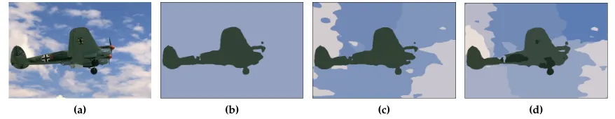
image and its segmentation intok=2, 5, 10 regions is shown in Figure 3. In this figure, for eachk,
the segmentation is represented as a color image with each pixel of a group labeled with the mean
color of its assigned region. This is a standard technique for visual and qualitative representation
of a segmentation.
[image:18.612.86.525.446.531.2](a) (b) (c) (d)
Figure 3:Example of segmented image. (a) Original image, (b)k=2, (c)k=5, (d)k=10.
II.4.1 Defining the Weight Matrix for Graph-based Image Segmentation
Image segmentation involves grouping pixels based on their color or feature characteristics, but
it also has the added complexity of being dependent on spatial location. Spatially close pixels
are more likely to come from the same physical object and should be more likely to be grouped
spatial and feature data vectors; however, this does not allow control over how much each type
of data influences the distance between pixels. It is also dependent on the ratio of the spatial
to feature dimension, which is dependent on the type of image. Instead, it is suggested in [10]
for graph-based image segmentation to compute the Gaussian weight matrix with the feature
coordinates multiplied by a Gaussian spatial window,
Wij=e
−kfi−fjk
2 2
σ2f · e−
ksi−sjk22
σs2 , ks
i−sjk2<r
0, otherwise
(II.6)
where {f1,f2, . . . ,fn} represents the normalized feature data of each pixel with fi ∈ Rw and
{s1,s2, . . . ,sn}represents the normalized spatial data of each pixel withsi ∈R2, andris a user
inputted distance. The feature data are normalized by the largest feature value, and the pixel
coordinates are normalized by the largest image dimension, ensuring that elements of fi andsi
are between 0 and 1. Note that the information included in the feature vector fi need not be
restricted to color/intensity values, but may include information like texture signatures, gradients,
and results of filtering techniques. The method of Equation II.6 captures the local relationships
between pixels by only considering points within anrradius of each pixel as related. A more
global approach is to define a single distance between pixelspi andpj to then use in the Gaussian
kernel of Equation II.3; i.e.,
d(pi,pj) = q
αksi−sjk22+ (1−α)kfi−fjk22, (II.7)
for α ∈ [0, 1]. This technique allows for control over the amount of spatial versus feature
information desired with the adjustment ofαwhile not restricting distances to a spatial domain.
Defining a data vectorxi= [
√
αsTi,
√
1−αfiT]Tfor each pixelpiallows the data setX={xi}ni=1,
xi∈Rw+2, to represent our image, with distances between points inXequivalent to Equation II.7.
This also gives the user the option of computing a full ork-nearest neighbors graph where only
the distances tokclosest neighbors of each point are kept in the weight matrix. We will represent
the image data as the above described data setXwhen computing Gaussian affinity matrices in
II.4.2 Image Segmentation Algorithms
Although image segmentation can be treated as a clustering problem, many algorithms have been
proposed and applied specifically to the image segmentation problem. Many of the fundamental
image segmentation algorithms are graph-based, and although they are very similar to the spectral
clustering methods of Section II.3, they are derived from a different perspective. Perhaps the most
well known is the Normalized Cut algorithm.
Let the image be represented as a undirected weighted graph G = (V,E) where the vertices
represent image pixels and the edges the similarity between the pixels, whose weights contained
in the affinity matrixW. To build the intuition behind the Normalized Cut algorithm, first consider
the case wherek=2; that is, we wish to partition the graph into two groups of verticesC1and
C2by cutting edges between these groups. Thecut cost, or cost for creating this partitioning is
defined as the sum of edge weightsWij of edges between the two groups:
cut(C1,C2) =
∑
xi∈C1,xj∈C2
Wij. (II.8)
The minimum cut is the partitioning of G that minimizes Equation II.8; however, this often
produces undesirable results by cutting a singleton point away fromG [31]. To overcome this
problem, the Normalized Cut cost
NCut(C1,C2) = Cut
(C1,C2)
Assoc(C1,V)
+ Cut(C1,C2)
Assoc(C2,V) (II.9)
can be minimized instead, where
Assoc(C,V) =
∑
xi∈C,xj∈V
Wij (II.10)
is theassociation cost, or total degree ofC. Normalizing by the total degree of each cluster makes
the minimum of the above NCut cost has been shown to be equivalent to
min y
yT(D−W)y yTDy
subject to yi ∈ {1,−β},i=1, 2, . . . ,n, (II.11)
yTD1=0,
where D is the diagonal degree matrix containing the row sums of W, di = Dii = ∑jWij,
β= (∑zi>0di)/(∑zi<0di),y= (1+z)/2−β(1−z)/2, andzis ann-dimensional indicator vector
wherezi=1 if vertexxiis inC1andxi=−1 ifxi is inC2. Finding the solution to Equation II.11
is NP-hard, but by relaxing the binary constraint onyby allowingy ∈ Rn, the solution of this
relaxed problem becomes equivalent to solving the generalized eigenvector problem
(D−W)y=λDy (II.12)
for the generalized eigenvector corresponding to the smallest non-trivial eigenvalue. Since we
allow components ofy to take on continuous values, a clustering algorithm such ask−means
must be applied to the eigenvector to assign a discrete labeling, howeveryis close enough to the
solution of Equation II.11 that this can now be done easily.
Remembering back to Section II.3, the solutionYof the Laplacian Eigenmaps objective function of
Equation II.4 is given by thekeigenvectors corresponding to theksmallest nontrivial eigenvalues
of Equation II.12 as well. This implies that fork=2, the solution to the Laplacian Eigenmaps
embedding problem is identical to that of the relaxed version of the NCut problem to optimally
cut a data set in two. This provides a natural extension for partitions intokclustersC, where we
can define the multiway cut and normalized cut [24] respectively as
Cut(C) = 1
2 k
∑
l=1
cut(Cl,V\Cl), (II.13)
NCut(C) = 1
2 k
∑
l=1
cut(Cl,V\Cl)
Assoc(Cl,V)
. (II.14)
The minimization of Equation II.14 can be relaxed into a form that is equivalent to the k
-dimensional Laplacian Eigenmaps problem, which has a solution that can be found from the
k-clustering is then found by applyingk−means clustering to thek-dimensional embeddingY, just as in the spectral clustering algorithm of Section II.3.
II.4.3 Superpixel Representation
Image segmentation is also complicated by the vast number of pixels in most images. Since each
image pixel is considered a vertex in the graph representation, ifnis the number of image pixels
then spectral clustering requires computing ann×ngraph Laplacian matrix with potentiallyn2
nonzero elements and then performing an eigendecomposition. This becomes computationally
prohibitive with medium to large images for most computers. Even if aK-nearest neighbors graph
is used, guaranteeing a Laplacian matrix havingO(kn)nonzero entries, sparse solvers may still
have problems for large images with hundreds of thousands or millions of pixels. To simplify the
complexity of the problem, small spatial regions of similar featured pixels calledsuperpixelscan be
identified and used to form vertices of a smaller graph that can be used for clustering. Letting
S ={S1,S2, . . . ,Sb}be the partitioning ofXinto superpixels, the reduced superpixel feature data
set becomesFS ={fSi}and spatial data setSS ={sSi}, where
fSi =
1
|Si|x
∑
j∈Sifj, (II.15)
sSi =
1
|Si|x
∑
j∈Sisj. (II.16)
Since these regions contain similar pixels, these sets of mean feature and spatial vectors of each
superpixel are still a good representation of the original data set. Similarly to Section II.4.1, we
can represent this as a reduced data set Xr = {xri}
b
i=1 with xri = [
√
αsTS i,
√
1−αfST
i]
T so that
Euclidean distances between points inXr are equivalent to the desired feature-spatial distance
of Equation II.7. In the context of images,Xr will represent the superpixel data set and in later
sections will represent the reduced data set for any type of data set.
Superpixels have been applied successfully to target detection [25], anomaly detection [20], and
image segmentation [17], as well as many other problems. The power of superpixels is the ability
to represent an image by a few thousand superpixels instead of hundreds of thousands of pixels
which allows for reasonable computation of these complex computer vision tasks. Superpixels are
also intimately related to image segmentation as the approximately equal sized superpixels can be
Figure 4:Examples of superpixel calculation using SLIC algorithm. By columns, Left: Original
image, Middle left: Outlines of region size 10 superpixels, Middle: Region Size 10
superpixels displayed with average color and mean position as black dot, Middle right:
Outlines of region size 20 superpixels, Right: Region Size 20 superpixels displayed with
average color and mean position as black dot.
A fast and robust algorithm for computing superpixels is the Simple Linear Iterative Clustering
(SLIC) [16] method, which creates image superpixels based on user-provided size and shape
parameters. The region size is specified as the approximate side length of the desired superpixels,
so for example a region size of 10 gives superpixels that contain around 100 pixels each. An
implementation of this method for use in MATLAB is publicly available in the VLfeat Toolbox
[23]. Examples of images, their SLIC superpixel regions, and the mean representation for different
region sizes are shown in Figure 4. The first column shows the original RGB image, the second and
fourth columns shows the outlines of each superpixel for a region size of 10 and 20 respectively,
and the third and fifth column displays the image with each superpixel assigned its mean color,
with a black dot representing the mean position of that superpixel for region size 10 and 20
respectively.
When computing a segmentation using superpixels, the data embedding is created for the reduced
superpixel data set instead of the full image data set. Since the desired output is a segmentation of
the original image, labels must be assigned to all pixels using only the knowledge of the reduced
data embedding. The simplest method of doing this would be to performk-means clustering
on the superpixel data embedding, and assign each pixel the label of its containing superpixel.
This however gives very chunky regions since superpixels do not perfectly conform to object
10.
III.
L
ongest
-L
eg
P
ath
D
istance
U
ltrametric
III.1
Definition
LetG = (V,E) be an undirected graph consisting of the set of verticesV and edgesE, and let
u,v∈V. LetPu,vbe the set consisting of all pathspiconnectinguandvinG, wherei∈ {1,· · ·,L}
withLrepresenting the total number of unique paths. Note that sinceG is undirected,Pu,v=Pv,u.
Each pathpi consists of a series edgespi={ei,1,ei,2, ...ei,Ki}representing the edges traversed by
that path, withei,j∈E. The longest-leg path distance (LLP-distance or LLPD) between verticesu
andv is defined as the minimum of the maximum weight edges of all paths connectinguand
v,
dll(u,v) = min pi∈Pu,v
max ej∈pi
w(ej) (III.1)
Thus, no matter which path is chosen betweenuandv, or equivalently betweenvandu, an edge
of weight at leastdll(u,v)must be traversed. A similar concept in graph theory is the Bottleneck
Edge Query (BEQ) problem which involves finding the maximum of the minimum edge weights
of paths of between two vertices. Since the graph adjacency matrix is computed from a Gaussian
Kernel, finding the LLP-distances on a graphG0= (V,E0)with the same vertices asGand edges
weighted based on Euclidean distance is equivalent to solving the Bottleneck Edge Query (BEQ)
problem on the graph adjacency matrix followed by a conversion via a logarithm.
An important quality of the LLP-distance is that it is an ultrametric, meaning it satisfies a stronger
version of the triangle inequality given by
dll(u,v)≤max{dll(u,w),dll(w,v)}, (III.2)
withu,v,w∈V. This provides the foundation for many theoretical guarantees for the outcomes
of unsupervised graph clustering using the LLP-distance as the metric in the exponent of the
Gaussian Kernel of Equation II.3 [1].
Ultrametrics naturally induce hierarchies because of this stronger version of the triangle inequality,
and hierarchies naturally induce an ultrametric [13]. The distances discussed in Section II.2 on
hierarchical clustering all obey this property, and actually the LLP-distance is closely related to
single linkage clustering. The LLP-distance between two points can be though of as the
III.2
Prior research
The LLP-distance was first introduced for use in clustering problems by Fischer et. al. [4], creating
the field of path-based clustering. The LLP-distance is used to define a clustering cost function
which is then minimized by an Iterated Conditional Mode algorithm using multi-scale techniques
to improve computational performance. This algorithm was shown to outperform other concurrent
top agglomeration methods on artificial data sets as well as segmentation of textured images. This
algorithmic framework was later modified to include automatic outlier detection by inclusion of
an outlier class, which was shown to perform well for edgel grouping and textured data [3].
In a later publication, Fischer et. al. proved that the LLP-distance is an ultrametric and thus
the matrix of LLP-distances was shown to induce a Mercer’s Kernel [5]. This allows for an
approximation of the path-based clustering result by applying k-means clustering to a lower
dimensional embedding of path-based distances using Kernel Principle Components Analysis. This
technique has the advantage of de-noising the hierarchy created by their previous agglomerative
method, leading to a more robust method. This also lead the way for path-based spectral
clustering.
Since path-based distances have the disadvantage of being heavily affected by noisy data points, a
robust path-based similarity measure was introduced in [8] based on M-estimation which lessens
the effect of outliers. This similarity measure was then used to define the affinity matrix for both
supervised and unsupervised spectral clustering. This method was tested on difficult artificial
data sets, image grouping of hand written digits and faces, and image segmentation of color
images, with promising results reported.
Theoretical guarantees of LLP-distance based spectral clustering have been proven under the
low-dimensional large noise (LDLN) data model, which assumes clusters are high density sets
separated by lower density regions of noise or outliers [1]. In this model, points with large
LLP-distance to theirKthnearest LLPD nearest neighbor are considered noise and are removed.
LLP-distances are then recomputed on the denoised data set before spectral clustering. It was
shown that given this data model, the largest eigengap of the symmetric LLPD Laplacian correctly
estimates the number of appropriate clusters as the number of eigenvalues before this gap. It was
also proved that the embedding of the data according to the symmetric LLPD Laplacian followed
by k-means clustering correctly labels most data points [1]. This brings improvement over using
the standard Euclidean distance between data points to create the affinity matrix which does not
III.3
Computation
In order to compute a spectral clustering, ann×nmatrix of distances is required, where nis
the total number of data points. When employing the LLP-distance, this is referred to as the All
Points Path Distance (AAPD) problem. The AAPD problem has been solved previously with the
algorithm of Floyd withO(n3)complexity [4], and can be solved using bottleneck spanning trees
using a modified SLINK algorithm withO(n2)complexity [1]. There exist theoretical methods
using bottleneck spanning trees with complexityO(nlogn), but numerical implementations of
these methods are currently not publicly available. There is however an easily implemented
algorithm to approximate the LLP-distance for a set of high dimensional data introduced in [1]
withO(nlogn)complexity. Due to the flexibility and efficiency of this approximate method, we
employ a modified version of this algorithm to calculate LLP-distance matrices in the experiments
of this thesis.
This fast approximate method represents the data points theoretically as vertices on a complete
graphGwith edge weights given by the Euclidean (L2) distances between vertices. Since computing
the complete graph would be computationally expensive for most data sets, a spanning tree ˜Gof
the complete graph is created instead by computing the edges corresponding to theK1-nearest
L2 neighbors of each vertex. It is assumed thatK1is chosen large enough to induce a spanning
tree ofG, with it being sufficient for this algorithm to chooseK1only large enough to induce a
minimum spanning tree.
Next, a set ofmthresholdst1<t2<· · ·<tmare chosen between the maximum and minimum
edge weights of ˜G, which are used to create a series of subgraphs of ˜G, denoted ˜Gts, containing
only edges of weight less thants. The LLP-distance between two verticesu,v ∈V can then be
approximated by finding the thresholdts at which two separate path connected componentsC1
andC2, withu∈C1andv∈C2, merge. That is, we assigndll(u,v) =ts, which is approximating
the minimum weight edge separating these two clusters. Since all intra-cluster edges at this stage
have edges of weight less than or equal tots, the clusters are connected and any further edges
joining the two clusters will have weight greater than or equal tots. It thus intuitively makes
sense thatts represents the minimum of the maximum edges separating anyu∈C1andv∈C2.
The algorithm is set up to find a vertex’sK-LLPD nearest neighbors by computing and sorting a
representation of each thresholded graph’s connected components.
We use a small generalization of this algorithm by approximating the LLP-distances using an
arbitrary L2 distance matrixDL2instead of theK
L2-distance matrix to be inputted if the size of the data set allows, and a knn-graph if the data
set is too large. Pseudo-code for our modified fast approximate LLPD algorithm is shown in
Algorithm 1. This algorithm works by computing ann×1 list of connected components for each
of subgraph described above and placing in the columns of ann×mmatrixCC. The rows of
CC are then sorted by column from left to right, which simulates a hierarchical clustering by
organizing all rows in the same connected component together at each stage. Therefore starting at
some row and traversing the first column ofCCsortedup or down will show if those points are in
the same connected component. If they are, thistsis the approximate minimum weight separating
those two data points. If they are not, then these points are still not in the same cluster, so we look
at the next row representing a higher thresholdts+1and check if this point is in the same cluster.
This process is continued untilKnearest neighbors are found. Note that ifK=na full matrix of
approximate LLP-distances will be returned.
Algorithm 1Modified Fast Computation of Approximate LLPD
Input:X,DL2,{ts}ms=1,K
Output:n×n Kapproximate LLPD-nearest neighbors matrix ˆDll
1: Allocaten×mmatrixCC.
2: fors=1 :m
3: Form matrixDts containing elements ofDL2less thants, zeros elsewhere.
4: Compute connected components ofDts storing insthcolumn ofCC.
5: end
6: Sort the rows ofCC by column from right to left to createCCsortedand let π(i)denote the
corresponding point order.
7: fori=1 :n
8: NN = 1 (number of nearest neighbors found)
9: iup=1,idown=1 10: fors=1 :m
11: whileCCsorted(iup,s) =CCsorted(iup−1,s)andNN<Kandiup>1 12: iup=iup−1
13: Dˆπll(i),π(i
up)=ts 14: NN=NN+1
15: end
16: whileCCsorted(idown,s) =CCsorted(idown−1,s)and NN<Kandidown>n 17: idown=idown+1
18: Dˆπll(i),π(i
down)=ts 19: NN=NN+1
20: end
21: end
III.4
Advantages and disadvantages for use in spectral clustering
Many clustering algorithms, including spectral clustering, have the disadvantage of poor
perfor-mance on non-convex and highly elongated clusters. This is due to points in the same cluster
being considered far apart in the Euclidean sense even if there is a high density of points between
signifying they belong to the same cluster. The LLPD is able to overcome this problem, since
points in high density clusters have small LLP-distances no matter the shape of the cluster.
(a) (b) (c)
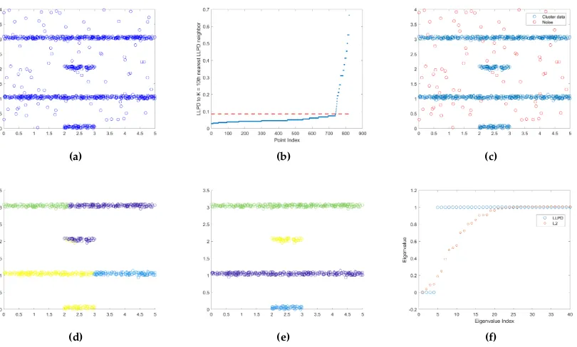
[image:29.612.107.512.234.478.2](d) (e) (f)
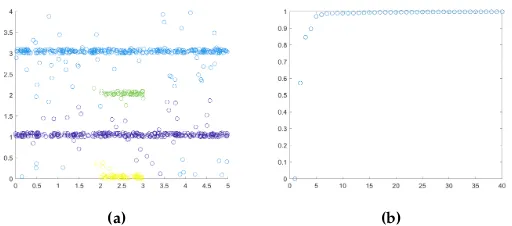
Figure 6:(a) Four Lines Data Set, (b) Plot of each point’s K = 10th LLPD nearest neighbor in
ascending order, points withKth LLPD nearest neighbor distance above the red line
are considered noise and removed, (c) Plot of data with noise as red circles and cluster
data as blue circles, (d) L2 clustering results, (e) LLPD clustering results, (f) 40 smallest
eigenvalues for L2 and LLPD embedding.
For example, consider the Four Lines data set from [1] in Figure 6, where points in two-dimensional
space are positioned in four elongated lines with low density noise between. Computing each
point’sK=10thnearest LLPD-neighbor and finding the elbow point when plotted in ascending
order gives an estimate of which points are outliers. These points are removed from the data
set, then the clustering is done on the remaining data. Using L2-distances to create the Gaussian
instead of keeping the high density clusters together. Spectral clustering using the LLPD Gaussian
weight matrix however yields a more accurate clustering. The LLPD clustering also has the
advantage that the correct number of clusters is clearly shown by the number of eigenvalues
before largest eigengap, whereas for the L2 clustering there is no large eigengap. This process is
outlined in Figure 6.
If instead clustering is performed on the Four Lines data set without denoising, the four lines are
still pulled out as separate clusters with noise getting assigned to one of the four clusters, shown
in Figure 7a. Although the correct clusters are identified, the largest eigengap no longer suggests
the correct number of clusters, shown in Figure 7b. Therefore the denoising process is still useful
for this data set in order to guarantee the eigengap property, and would be more necessary in
data sets with distinct outliers versus low density noise as with this data set.
[image:30.612.179.435.312.425.2](a) (b)
Figure 7:(a) LLPD clustering results without denoising, (b) 40 smallest eigenvalues for LLPD
embedding without denoising.
The LLP-distance has the disadvantage of sensitivity to noise and outliers [29], especially structured
noise and clusters that are much denser than others [1]. For example, consider the data set in
Figure 8, composed of two boomerang shaped clusters. Choosing one data point, the LLPD and
L2 distances from this point to all other points are calculated and plotted by color in Figures 8a
and 8b respectively. The LLP-distances alone suggest two clusters, while the L2 distances do not
provide such a crisp boundary. Adding ten points along the liney=x+ewhere x∈[.1, .7]and
e∈[−.02, .02]are randomly chosen, the same two plots are created in Figures 8c and 8d. With
these few added points of structured noise, the scale of the LLPD changes dramatically, and causes
the two clusters to no longer be distinctly separable visually, showing that the addition of just
a few well placed data points can affect the LLPDs of the entire data set. Although all sets of
random noise chosen along this line may not give such drastic changes in the LLP-distances of
An advantage of the L2 distance is that the scale of distances and distances to non-noise points
remains the same with the addition of the noise, so only 10 new distances need to be calculated,
whereas all LLPDs must be recalculated.
[image:31.612.95.521.156.244.2](a) (b) (c) (d)
Figure 8:Comparison of L2 to LLPD from the pointp = (1.1910, 0.2114)in an artifical data set
with and without noise. (a) L2 distances frompwithout noise, (b) LLPD from pwithout
noise, (c) L2 distances frompwith 10 added data points of noise, (d) LLPD distances
IV.
P
ath
-
based
C
lustering
D
enoising by
P
re
-
cluster
A
veraging
We propose a novel LLPD-based clustering scheme that reduces the influence of noise on the
spectral data embedding as well as the size of the eigendecomposition problem while maintaining
accuracy.
IV.1
Motivation
The noise removal method introduced in [1] relies on identifying and removing potential outliers
before computing the spectral clustering. This method been shown to be effective on a number of
artificially created data sets as well as the DrivFace data set [12]. These data sets are all composed
of a set of discrete data points, however for other types of data the strict removal of data points
becomes more problematic. For example, consider a data set of pixels of an RGB or hyperspectral
image where both a spectral as well as a spatial component are important to segmenting relevant
regions of the image. Removing data points in this instance amounts to removing pixels in the
image which complicates the spatial component of similarity as well as the continuity of the
final segmentation. This is also quite computationally expensive since images generally contain
hundreds of thousands of pixels. We thus are looking for a way of negating the effect of noise on
a path-based distance metric without removing the noise.
Assuming the data set is composed of high density clusters with relatively uniform low density
noise, an initial coarse clusteringCinit={c1,c2, . . . ,cb}of approximatelyequal-sizedpartitions of
the data should each contain about the same number of noise points, withk bn. These
"pre-clusters"ciwill be mostly composed of non-noise data points with a few noise data points
each due to the low density of noise points. The average of the data points of each initial cluster
¯
ci = (1/|ci|)∑xj∈cixj will thus largely reflect the data points of the desired clusters and not the
noise. We then can define these averages of the initial clusters as points in a new reduced data set
Xr ={c¯1, ¯c2, . . . , ¯cb}which reflect the relevant characteristics of the full data set, and calculate the
embeddingYr ∈Rb×kon this smaller data set. Using this embedding, we can then transfer this
information back to compute an embeddingY∈Rn×kof the full data set.
We illustrate this with three artificial data sets in Figure 9 and show that, using this alternative
denoising technique, the appropriate clusters are identified. The first data set is the Four Lines
data set of Figure 6, the second is the Nine Gaussians data set introduced in [1] composed of
deviation, and the last is composed of three intertwined arcs of data points. All data sets have
uniform low density random noise inserted. Each data set is reduced by performingk-means
clustering and merging clusters until all are of approximately equal size, shown in the second
column of Figure 9. An LLPD spectral clustering is then applied to each reduced data set seeking
[image:33.612.97.518.253.491.2]the appropriate number of clusters, that isk=4, 9, 3 respectively, shown in the third column of
Figure 9. We then extend this clustering to the full data set by naively assuming that allxj ∈ci
should be assigned the same label asci, shown in the last column of Figure 9. From the results
of these three toy problems we can see that this method yields the correct clusters, assigning the
noise to a nearby cluster.
Figure 9:Clustering by preclustering on three artificial data sets: Four Lines (Row 1), Nine
Gaussians (Row 2), and Three Arcs (Row 3). Columns left to right: Original data set,
pre-clustering reduced data set, LLPD clustering of reduced data, corresponding LLPD
clustering of original data.
For an image, we can decompose the hundreds of thousands of uniformly spaced pixels into a
few hundred or thousand superpixels, represented by the mean color and spatial location of all
containing pixels. The superpixel segmentation will be used as the preclustering step for our
new denoising method described above. We test this on the 50×50 pixel artificially created RGB
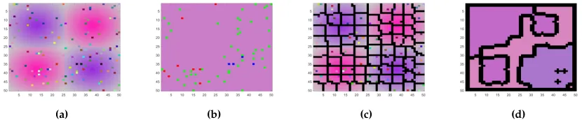
image of Figure 10a. The image is composed of four square regions of Gaussian shaped pink or
purple squares should be identified, and withk=4 segments the four separate squares should be
identified. Performing LLPD spectral clustering withk=4 on the full image without any noise
reduction causes three of the segments to be composed of noise, represented by red, green, and
blue in Figure 10b for clarity, and the fourth segment containing all other pixels, represented by
their average color in Figure 10b. This is very far from the desired segmentation of the four square
regions, and shows how affected by noise segmentation, and especially path-based segmentation
can be. The image is then divided into approximately 6×6 superpixels, visualized in Figure 10c
with black lines showing the outlines of the superpixels. A new segmentation is then calculated
from the set of averaged superpixel data, and all pixels in a superpixel are given the label of that
superpixel. This is displayed in Figure 10d by giving each segment its average color and outlining
the segment boundaries in black. The segmentation in Figure 10d is still not ideal, but is able to
capture the main structure of the image with only one class getting lost to noise.
[image:34.612.99.514.322.408.2](a) (b) (c) (d)
Figure 10:(a) Original Image, (b) LLPD segmentation of full image without noise reduction for
k = 4 segments, with the background class represented by average color and three
noise classes represented by red, green, and blue for clarity (c) Superpixel visualization
of approximately 6×6 pixels each, (d) LLPD segmentation using superpixels of (c)
fork=4 segments. Using superpixels allows for the main structure of the image to
be visible after segmentation whereas segmentation of the full image identifies noisy
pixels as clusters.
These simple artificial examples show that pre-cluster averaging can be a viable way to compute
an embedding robust to noise. In these examples we made the simple assumption that all points
in a pre-cluster should be assigned the same label as the pre-cluster data point in the reduced
model. For more complex and noisy data sets, this simple assumption will give coarse and
unsophisticated segmentations, such as very blocky region borders in images (see Figure 5). This
also does not guarantee that the embedding at each image pixel will be the same embedding
coordinates as the full non-noisy image computation. Therefore we explore various methods of
appropriate clustering of the full data set.
IV.2
Out-of-sample extension of a Laplacian-Eigenmaps embedding
A large burden of spectral graph-based clustering methods is the necessary computation of a large
square weight matrix and its eigendecomposition. For large data sets this becomes computationally
prohibitive quickly as the size of the data set grows. Therefore, methods that make use of a smaller
data set for the bulk of the computations, then extend this information back to the full data set are
needed. This type of method is also useful for data sets that are continually growing, so that with
each new data input a new model does not have to be created.
An out-of-sample extension for unsupervised graph-based spectral techniques was introduced in
[26]. This method based on the Nyström extension formula [7] can be used to extend the results
from Multi-Dimensional Scaling (MDS) [19], Laplacian Eigenmaps (LE) [11], Isomap [9], and Local
Linear Embeddings (LLE) [18]. These methods are all based on computing a low-dimensional
representation of a set of data points from the eigenvectors of a symmetric matrix, with each using
a different matrix. The steps and notation for this common framework can be described as
1. Given a data setX={x1,x2, . . . ,xn}withxi ∈Rm, construct ann×nsimilarity (adjacency)
matrixM, with each entryMij=KX(·,·)defined by a symmetric functionKX :(Rm×Rm)→
R,
2. Compute the matrixV = [v1, . . . ,vk]T containing the eigenvectors ofMcorresponding to
theklargest positive eigenvaluesλ1, . . . ,λk and define the vectorλvec= [λ1, . . . ,λk]T,
3. Letyi represent theithcolumn of the matrixV. The embeddingei∈Rk of data pointxi ∈X
is ei = yi for LE and LLE, andei = λ1/2vec yi for MDS and Isomap where represents
pointwise multiplication.
Note that in Section II.3, the LE embedding solution was given by the eigenvectors corresponding
to theksmallest nontrivial eigenvalues of a generalized eigenvector problem. This is an equivalent
result up to a componentwise scaling to the solution described by the above framework using the
normalized adjacency matrix [28].
Now consider a pointx∈Rm, withx ∈/X, that we would like to embed as a new pointy∈Rk.
Ideally this should be done so that the relation betweenxand allxi ∈Xis captured in the relation
converge to an eigenfunction. Therefore, a linear operatorKρoperating on functions in a Hilbert
spaceHρof densityρ(x)can be associated with kernelKX forg∈ Hρas
(Kρg)(x) =
Z
KX(x,y)g(y)ρ(y)dy. (IV.1)
The actual density ρ(x)is unknown given our limited data set, so IV.1 must be approximated
using the empirical distribution ˆρgiven by the data inX. Using these ideas, it is shown in [27]
that using the empirical distribution ˆρ, thek×1 embedding coordinateyfor LE and LLE of the
new pointxis given componentwise by
ej =yj= 1
λj n
∑
i=1
VjiKX(x,xi), (IV.2)
which gives a single real valued number, and is calculated for j = 1 to j = kthen stacked to
form the embedding coordinatey == [y1,y2, . . . ,yk]T. For MDS and Isomaps, the embedding
coordinate componentwise isej =
q
λjyjas before.
IV.3
Spatial-smoothing techniques for out-of-sample image segmentation
Denoising by superpixel averaging causes the superpixel embedding to be relatively unaffected
by noise, so that when extended to non-noise image points via the out-of-sample extension, the
"correct" embedding coordinates are calculated. When the superpixel embedding is extended to
noise points however, the resulting embedding of those points are still noisy since the superpixel
embedding will not represent them well. This may seem counterintuitive since we are claiming
this method is robust to noise, however the distinction between this method and previous is that
theunderlying embeddingto be extended is robust to noise, whereas performing the embedding with noisy points results in the entire embedding being tainted, as shown earlier in Figure 10. Our
new technique therefore allows the underlying embedding of the superpixels to be true to the
main features of the image.
Therefore, since noise points are not embedded well by the extension, the final segmentation
will be composed of spatially incoherent segments. Desired segments however are generally
composed of spatially neighboring pixels representing physical objects in the image. To overcome
two-dimensional convolution operator that is used to smooth or "blur" an image, given pixelwise
by
˜
pi=
∑p∈Ωi f Gˆ (p,pi)
∑p∈ΩiG(p,pi)
(IV.3)
where ˆf represents the vector pixelp (either the feature vector for smoothing the image or the
embedding vector for smoothing the final embedding),Ωi is a square spatial window around
pixelpi, andG(p,pi)is the two-dimensional Gaussian distribution given by
G(p,pi) = 1
2πσ2e
−(x−xi)2+(y−yi)2
2σ2 . (IV.4)
where xandy represent the spatial location of pixel p, andxi andyi represent the location of
pixelpi.
IV.4
General algorithm for image segmentation
In order to calculate the out-of-sample extension of Equation IV.2, the value of the LLPD Gaussian
kernel must be computed between each point of X and Xr. This could be computed by first
finding the LLP-distances using Algorithm 1 for the data set{X,Xr}, however this would be
computationally expensive and only distances between the two groups of data points are needed.
Instead, we can simply use theCCmatrix computed usingXr in Algorithm 1 by adding a row for
the new data point ofXbeing considered, connect this point to each graph representation ofXrat
levelts with any new edges, and merge any distinct connected components that have been joined
by new edges. The same method of finding nearest neighbors as Algorithm 1 is then employed for
the newly added point only. This method is outlined in Algorithm 2 with pseudocode. Combining
this with the ideas of the previous three sections, we present the framework for computing an
image segmentation using the LLPD and superpixel denoising with extension method. The overall
process is shown by the flow chart of Figure 11, with each step written in detail below:
1. Inputp×q×wimageIand calculate pixel data setX={xi}withxi= [
√
αsTi,
√
1−αfiT]T.
Optional: Perform pre-spatial smoothing on input imageI.
2. Calculate the b SLIC superpixels S = {S1,S2, . . . ,Sb} of I and create the reduced data
setXr ={xri}
b
Figure 11: Flowchart of superpixel denoising with extension method.
xri = [
√
αsTS i,
√
1−αfST
i]
T.
3. Create adjacency matrix W of Xr using Gaussian kernel, Wij = e
−kxi−xjk
2
σ2 . Use to form
diagonal degree matrixDii=∑jWij.
4. Solve the generalized eigenvector problem(D−W)v=λDvfor thekeigenvectorsv1,v2, . . . ,vk
corresponding to theksmallest eigenvaluesλ1≤λ2≤. . .≤λk.
5. Form the spectral embedding ofXr given by the columns ofV= [v1,v2,· · ·,vk]T.
6. Calculate the LLPD of each xi ∈ X to each xrj ∈ Xr using Alg. 2. That is b distances
dll(xi,xrj)for eachxi. Form kernel from each distanceKX(xi,xrj) =exp(−
dll(xi,xrj)2
σ2 ).
7. Use out-of-sample extension to calculate the k×1 embedding y of each x ∈ X given
componentwise byyi= λ1i∑bj=1VijK(x,xrj).
8. Compute k−means clustering on final image embedding yi to compute segmentation.
Algorithm 2Compute LLP-distances to new point in reduced data set
Input:CC,x,Xr,{ts}ms=1Output:List of distances to new pointx,Dll,x
1: Add zero row to bottom ofCC.
2: Calculateb×1 vectorDn,xof L2 distances ofxto allxi ∈Xr.
3: fors=1 :m
4: Calculate indicator vector ˜Dn,xof entries inDn,x<ts.
5: ifD˜n,xcontains nonzero entry(s)
6: Find which connected component each nonzero entry corresponds to: nbrs=CC(s, ˜Dn,x).
7: Merge all components of nbrs into one component
8: Add merge component number to last row of columns.
9: else
10: CC(s, end) =max(CC(s, :)) +1.
11: end
12: end
13: CalculateCCsortedby sorting rows of CC by column, withπ(i)denoting the corresponding
point order.
14: startingPoint=π(n+1)% row ofCCcorresponding to the new point
15: Compute lines 7-21 of Alg. 1 for i=startingPoint,K=n+1, storing distances inDll,x.
16: end
IV.5
Linear interpolation of superpixel embedding
A less sophisticated method of extending a superpixel embedding to the full pixel grid is to
perform a linear interpolation of the superpixel embedding over the spatial coordinates of all
pixels. That is, letSibe theithsuperpixel andNibe the set of superpixels that are adjacent spatially
to superpixelSi as well asSi. A linear interpolationFi is then created such that forS∈N,
Fi(sS) =yS (IV.5)
where sS is the average spatial location of superpixel S and yS represents the embedding of
superpixelS. Now that this function has been created, for every pixel pi ∈ S, the embedding
of that pixel is given byFi(spi)wherespi is the spatial location of pi. A different interpolation
functionFi is then created for each superpixelSi, giving an embedding coordinate for every pixel
in the image.
This method allows us to assign each pixel an embedding coordinate that transitions smoothly
Figure 12:Normalized cut image segmentations using superpixels fork=5. First row: original image, Second row: each pixel is assigned the label of its superpixel, Third Row:
Interpolating of the superpixel embedding over the spatial coordinates of the image.
yielding segmentations with smoother boundaries compared to assigning each pixel the label of
its superpixel, as seen in the third column of Figure 12. Even using this interpolation method,
object boundaries are not captured with high accuracy since the interpolated embedding is not
equal to the true embedding of the image.
Unlike the out-of-sample extension method described in the previous sections, the interpolation
method does not guarantee the convergence of the embedding coordinates as the number of
samples grow. This method does however still benefit from the denoising by superpixel averaging
outlined in Section IV.1, and is much less computationally expensive. Therefore we provide it as a
viable alternative and will compare the more mathematically founded out-of-sample extension
V.
I
mage
E
xperiments and
R
esults
V.1
LLPD in images
Image segments are separated by boundaries called contours, often represent