A Study On Short Term Load Forecasting

UNIVERSITI TEKNIKAL MALAYSIA MELAKA (UTeM)

FACULTY OF ELECTRICAL ENGINEERING

FINAL REPORT (PSM 2)

NAME: MOHD ZULHAFIZ BIN MOHD JOHARI

MATRIC NO: B010510164

COURSE: 4 BEKP

“I hereby declare that I have read through this report entitle “a study on short term load forecasting” and found that it has comply the partial fulfillment for awarding the degree of

Bachelor of Electrical Engineering (Industrial Power)”

Signature : ………..

Supervisor’s Name : ELIA ERWANI BTE HASSAN

A STUDY ON SHORT TERM LOAD FORECASTING

MOHD ZULHAFIZ BIN MOHD JOHARI

A report submitted in partial fulfillment of requirements for the degree of bachelor in electrical engineering (industrial power)

Faculty of Electrical Engineering

UNIVERSITI TEKNIKAL MALAYSIA MELAKA

I declared that this report entitle “a study on short term load forecasting” is the result on my own research except as cited in the references. The report has not been accepted for any degree and is not concurrently submitted in candidature of any other degree.

Signature : ………

Name : MOHD ZULHAFIZ BIN MOHD JOHARI

v

ACKNOWLEDGEMENT

Bissmillahirahmanirahim. In the name of Allah S.W.T, the most gracious and

merciful, praise to Allah the lord of universe and may blessing and peace of Allah be upon his messenger Muhammad S.A.W. Thanksgiving to Allah because He has give me opportunity to complete my final year project and final year report. Without His blessing, I sure can’t complete this task in the time given.

First and foremost, my sincerest appreciation must be extended to the Elia Erwani

bte Hassan who has gives me opportunity to complete my final year project under her supervision. She have share all her experience, expertise and knowledge to help me complete my final year project. Her brilliant advices and guidance have helped me to complete this task successfully within the given time.

Apart of that, to my supportive friends who have helped me all the time during the process to finish the final year project and final year report. Those entire things happen because of brilliant idea, help and support from all my friends.

vi

ABSTRACT

vii

ABSTRAK

viii

TABLE OF CONTENTS

CHAPTER TITLE PAGE

ACKNOWLEDGEMENT v

ABSTRACT vi

ABSTRAK vii

TABLE OF CONTENTS viii

LIST OF TABLES xi

LIST OF FIGURES xii

LIST OF ABBREVIATIONS xv

LIST OF APPENDICES xvi

1 INTRODUCTION 1

1.1 Objectives 1

1.2 Problem Statement 1

1.3 Scope of Work 1

1.4 Background 2

1.4.1 Artificial Neural Network 2 1.4.1.1 The Components of ANNs 3 1.4.1.2 The Back Propagation Algorithm 4

2 LITERATURE REVIEW 5

2.1 Introduction 5

2.2 The Components of ANNs 5

2.2.1 Input and Output Factor 6

2.2.2 Weighting Factor 6

2.2.3 Neuron Model 7

2.2.4 Transfer Function 7

ix

2.2.7 Hidden Layers and Node 10

2.2.8 Learning Rate 10

2.2.9 Momentum Rate 10

2.3 Literature Review 11

2.3.1 Application of Neural Network to Load Forecasting in Nigerian Electrical Power System by G. A. Adepoju, S.O.A.

Ogunjuyigbe and K.O. Alawode, Ladoke Akintola University of Technology, Nigeria

(2007) 11

2.3.2 Short Term Load Forecasting based on Neural Network and Moving Average by Jie Bao, Department of Computer Science, Iowa State University, Ames, IA (2002) 14 2.3.3 Short Term Load Forecasting for The Holiday

Using Fuzzy Linear Regression Method by Kyung Bin Song, Member, IEEE,

Young-Sik Baek, Dug Hun Hong, and

Gilsoo Jang, Member, IEEE. 18

3 METHODOLOGY 22

3.1 Introduction 22

3.2 Network Structure 22

3.3 Pattern Data 24

3.3.1 Training Data 24

3.3.2 Testing Data 25

3.4 Flow Chart of Overall Process 25

3.4.1 Flow Chart of Training Process 27 3.4.2 Flow Chart of Testing Process 29

4 RESULT AND DISCUSSION 30

4.1 Single Network 30

x

4.1.1.1 The Network ANN Without

Indicator 31

4.1.1.2 The Network ANN With

Indicator 38

4.1.2 Testing Phase 48

4.1 Results for Load Forecasting 49

5 CONCLUSION AND RECOMMENDATION 54

REFERENCES 56

APPENDICES 57

xi

LIST OF TABLES

TABLE TITLE PAGE

2.1 Absolute Mean Error (%) 14

xii

LIST OF FIGURES

FIGURE TITLE PAGE

1.1 Black box device 3

1.2 Component of ANN 3

2.1 Basic Component of ANN 5

2.2 Simple summation function to determine the output 6

2.3 Summation function that is compared to the threshold to

determine output 7

2.4 The types of transfer function. (a) Hard limiter (b) Linear function

(c) Sigmoid function 8

2.5 Single layered neural network 9

2.6 Multilayered neural network 9

2.7 Average daily loads for August 2003 12

2.8 Plots of the ‘target’ and ‘forecast’ loads in MW values against

the hour of the day 13

2.9 The general neural network load forecasting 15

2.10 Forecasted result (hour-ahead model) 16

2.11 Forecasted error (percent) 16

2.12 Forecasted result (day-ahead model) 17

2.13 Forecasted error (percent) 17

2.14 The load differences between the peak loads of the four weekdays

before the Arbor Days and the peak loads of the Arbor Days during

xiii

2.15 Load differences between the peak loads of the four weekdays

before the Arbor Days and the peak loads of the Arbor Days

from the 1960s to 1990s. 20

3.1 Network structure of ANN without indicator 23

3.2 Network structure of ANN with indicator 24

3.3 Flow chart of overall process 26

3.4 Flow chart of training process 28

3.5 Flow chart of testing process 29

4.1 Changes in network parameter for the network without indicator

(a) Momentum rate (b) Learning rate (c) Epoch (d) Goal

(e) Hidden nodes (f) Training function 34

4.2 Changes in network parameter for the network without indicator

(a) Momentum rate (b) Learning rate (c) Epoch (d) Goal

(e) Hidden nodes (f) Training function 38

4.3 A single ANN with indicator. (a) The training performance

(b) Regression value 39

4.4 A graph of regression value when changes in network

parameters for the network with indicators. (a) Hidden nodes

(32,8,24) (b) Hidden nodes (32,4,24) (c) Hidden nodes

(32,1,24). 41

4.5 Changes in network parameters for the network with

indicators. (a) Learning rate (0.8) (b) Learning rate (0.99) 42

4.6 Changes in network parameters for the network with

indicators. (a) Momentum rate (0.3) (b) Momentum rate (0.7) 43

4.7 Changes in network parameters for the network with indicators.

(a) Epoch (500) (b) Epoch (1500) 44

4.8 Changes in network parameters for the network with indicators.

(a) Goal (1e-06) (b) Goal (1e-24) 45

4.9 Changes in network parameters for the network with indicators

xiv

(c) Training function (traingdm) (d) Training function (traingdx). 47

4.10 A graph of regression value when changes in network

parameters for the network with indicators. (a) Hidden nodes

(32,8,24) (b) Hidden nodes (32,4,24) (c) Hidden nodes

(32,1,24). 49

4.11 Plots of the ‘target’ and ‘forecast’ load in KW values against the 53

xv

LIST OF ABBREVIATION

TNB - Tenaga Nasional Berhad

STLF - Short Term Load Forecasting

ANN - Artificial Neural Network

MLP - Multilayer Perceptron

PE - Processing Element

AME - Absolute Mean Error

MW - Megawatt

ARMA - Automatic Regressive Moving Average

MV - Moving Average

xvi

LIST OF APPENDICES

APPENDIX TITLE PAGE

A Example of training program load data 57

CHAPTER 1

INTRODUCTION

1.1 Objectives

The objectives of this project are

1. To learn on short term load pattern based on data collection. The load data was

collected from Tenaga Nasional Berhad (TNB).

2. To forecast or predict the load flow for the next 24 hours for economic dispatch by

using ANN.

3. To develop ANN using back propagation method that will give a faster result

compared with conventional method.

1.2 Problem Statement

Nowadays, the electrical load increase about 3-7% per year for many years. At the

present time, conventional method gives a longer time to make a prediction. STLF is

important to supplier because they can use the forecasted load to control the number of

generators in operation either shut up some unit when forecasted load is low or start up of

new unit when forecasted load is high.

By using Artificial Neural Network, this project will show how to forecast or

2

1.3 Scope of Work

For this project, the scope covered on short term load forecasting (STLF). Short

term load forecasting means that the forecaster calculates the estimated load for each hours

of the day, the daily peak load, or the daily or weekly energy generation.

In this project, the load data in 3 month will be used in training and load data for

the next 3 month will be used in testing. The input load data will be load on Saturday,

Monday, Wednesday, and Friday. Meanwhile, the target load data will be load on Sunday,

Tuesday, Thursday, and Saturday. The parameter that used in this project are learning rate,

momentum rate, maximum number of iteration (epoch) and the minimum error goal. The

training performance must be 100 percent. If the 100 percent performance was not meet,

then the parameter will be adjusted to get the 100 percent performance during training.

The quality of training data, the initial weights used, and the network structure used

will give the performance and reliability of Artificial Neural Network (ANN). The trained

network can then make prediction based on the relationships learned during training.

1.4 Background

1.4.1 Artificial Neural Network

Artificial Neural Networks (ANNs) refer to a class of models inspired by the

biological nervous system.The models are composed of many computing elements, usually

denoted neurons and each neuron has a number of inputs and one output. It also has a set of

nodes called synapses that connect to the inputs, output, or other neurons. [1]

Most ANN models focused in connection with short-term forecasting use

multi-layer perceptron (MLP) networks. The attraction of MLP can be explained by the ability of

the network to learn complex relationships between input and output patterns, which would

3

A number of different models intended to initiate some function of human brain,

using certain part of it basic structure described as neural network. It consists of large

number of simple processing elements called neurons or nodes or simply processing units

which are interconnected to each other. It can also describe as black box device, processing

information coming in and producing a certain output. [2]

Figure 1.1: Black box device

1.4.1.1 The Components of ANNs

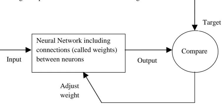
Commonly neural networks are adjusted or trained, so that a particular input leads

to a specific target output. Such a situation is shown below. There, the network is adjusted,

based on a comparison of the output and the target, until the network output matches the

target. Typically many such input or target pairs are needed to train a network.

Figure 1.2: Component of ANN Incoming

signal Output

4

1.4.1.2 The Back Propagation Algorithm

Back propagation was created by generalizing the Widrow-Hoff learning rule to

multiple-layer networks and nonlinear differentiable transfer functions. Input vectors and

the corresponding target vectors are used to train a network until it can approximate a

function, associate input vectors with specific output vectors, or classify input vectors in an

appropriate way as defined. The term back propagation refers to the manner in which the

gradient is computed for nonlinear multilayer networks. There are a number of variations

on the basic algorithm that are based on other standard optimization techniques, such as

conjugate gradient and Newton methods.

The simplest implementation of back propagation learning updates the network

weights and biases in the direction in which the performance function decreases most

rapidly, the negative of the gradient. One of iteration of this algorithm can be written as

Xk

+

=

-

α

g

where

X

g

CHAPTER 2

LITERATURE REVIEW

2.1 Introduction

This project will focus on application of Artificial Neural Network to forecast or

predict the load flow for economic dispatch. A set of load data is chosen in a case of

classification problem. The following studies were reviewed to gain an idea in doing this

report.

2.2 The Components of ANNs

Commonly neural networks are adjusted or trained, so that a particular input leads

to a specific target output. Such a situation is shown in figure below.

Figure 2.1: Basic Component of ANN

There, the network is adjusted, based on a comparison of the output and the target,

until the network output matches the target. Typically many such input or target pairs are

needed to train a network.

Neural Network including connections (called weights) between neurons

Compare Input

Adjust weight

Output

6

2.2.1 Input and Output Factor

During applying back propagation algorithm to the problem, selection of input is

very important part that has an impact on the desired output. If there is much input to a

neuron, there should be as many input signal in processing elements (PEs).

Selection input in improper will cause divergence, longer learning time and

inaccuracy reading, greater than 1.

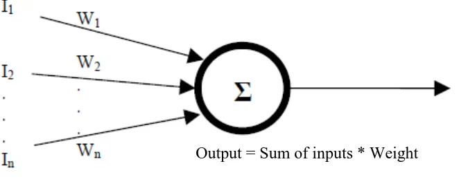
2.2.2 Weighting Factor

Relative weighting will be installing in each input and this weighting will affected

the impact the input as shown in Figure 2.2. Weights determine the intensity of the input

signal and are adaptive coefficients within the network. To various input, the initial weight

for PE can be modified and according to the network’s own rules for modification.

Figure 2.2: Simple summation function to determine the output

The inputs and the weights on the inputs can be seen as vectors mathematically,

such as (I1, I2 … In) and (W1, W2 …Wn). Each component of I vector by corresponding

component of the W vector and add up the entire product as an example input 1 = I1 * W1.

Then all these input are added to give the scalar result.

7

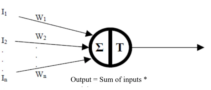
2.2.3 Neuron Model

A neuron also known as a processing element and several important activities take

place within the design of this processing element. The summation function was examined

first which is represented in Figure 2.2 and Figure 2.3. It will be more than a simple

summation after all products was summed and then was compared to some threshold to

determine the output. If the threshold is less than the sum of the output, the processing

element generates a signal. If the threshold is greater than the sum of the inputs, there is no

signal was generated.

Figure 2.3: Summation functions that is compared to the threshold to determine output

2.2.4 Transfer Function

There are many transfer function and basically the transfer function is a non-linear.

The linear also known a straight line and the linear function is limited because the output is

proportional to the input. Although, the output is depends upon whether the result of

summation is negative or positive. The network output can be 1 and -1, or 1 and 0.

The hard limiter transfer function was used in perceptrons to create neurons that

make classification decisions. For the linear transfer function, neurons of this type are used

as linear approximators in linear filters. The sigmoid transfer function takes the input

which can have any value between positive and negative infinity, and squashes the output

into the range 0 to 1.