On Brauer algebra simple modules over the complex field

City, University of London Institutional Repository

Citation

:

10.1090/tran/6716

This is the accepted version of the paper.

This version of the publication may differ from the final published

version.

Permanent repository link:

Link to published version

:

Copyright and reuse:

City Research Online aims to make research

outputs of City, University of London available to a wider audience.

Copyright and Moral Rights remain with the author(s) and/or copyright

holders. URLs from City Research Online may be freely distributed and

linked to.

City Research Online: http://openaccess.city.ac.uk/ publications@city.ac.uk

FIELD

MAUD DE VISSCHER AND PAUL P MARTIN

Abstract. This paper gives two results on the simple modules for the Brauer algebra

Bn(δ) over the complex field. First we describe the module structure of the restriction of all simpleBn(δ)-modules to Bn−1(δ). Second we give a new geometrical interpretation of

Ram and Wenzl’s construction of bases for ‘δ-permissible’ simple modules.

1. _Introduction

1.1. Classical Schur-Weyl duality relates the representations of the general linear group and the symmetric group via commuting actions on tensor space. The Brauer algebra was introduced by Brauer in 1937 to play the role of the symmetric group when one replaces the general linear group by the orthogonal or symplectic group. For any non-negative integer n, any commutative ring k, and any δ ∈ k, we can define the Brauer algebra Bn(δ) as being

the k-algebra with basis all pair partitions of 2n. We can represent these basis elements as diagrams (so-called Brauer diagrams) having 2n vertices arranged in 2 rows of n vertices each, such that each vertex is linked to precisely one other vertex. The multiplication is then given by concatenation, removing all closed loops, and scalar multiplication by δk where k

is the number of closed loops removed. It’s easy to see that Bn(δ) is generated by the set {σi, ei : 1≤i≤n−1}where σi and ei are given in Figure 1.

i i+1

i i+1

... ... ... ...

i i+1

i i+1

Figure 1

The symmetric group algebrakΣnappears naturally as the subalgebra ofBn(δ) generated

by theσi’s. Note that kΣnalso occurs as a quotient ofBn(δ) as explained below. This turns

out to be very helpful in studying the representation theory of Bn(δ).

Assume for a moment thatδis a unit. Consider the idempotent given bye= 1_δen−1. Then

it is easy to see that

eBn(δ)e∼=Bn−2(δ) and Bn(δ)/Bn(δ)eBn(δ)∼=kΣn. (1)

Now fix k=_C and recall that the simple _CΣn-modules are indexed by partitions of n, that

is for each partitionλwe have a (simple) Specht module Sλ_{. Using (1) we can easily deduce}

by induction on n that the simple modules forBn(δ) are indexed by the set Λn of partitions

ofn, n−2, n−4, . . .. For eachλ∈Λn, we denote the corresponding simple module byLn(λ).

WhenBn(δ) is semisimple, the simple modules can be constructed explicitely by ‘inflating’

(or ‘globalising’) the corresponding Specht module, see for example [8]. However the algebra

Bn(δ) is not always semisimple. In 1988, Wenzl showed in [17] that ifBn(δ) is not semisimple then δ∈_Z, and in 2005, Rui gave an explicit criterion for semisimplicity in [16].

In this paper, we study the simple modules when Bn(δ) is not semisimple. So we will

assume that δ ∈ _Z. For the moment we will also assume that δ 6= 0. In this case, Bn(δ) is

a quasi-hereditary algebra with respect to the opposite order to the one given by the size of partitions. (In fact, we will work with a refinement of this order, see Section 2.2). In partic-ular, the indecomposable projective modules Pn(λ) (λ ∈ Λn) have a filtration by standard

modules ∆n(λ) (λ ∈Λn). The standard modules can be constructed explicitly (as inflation

of Specht modules, as in the semisimple case) and we have surjective homomorphisms

Pn(λ)∆n(λ)Ln(λ)

for eachλ∈Λn. Now the decomposition matrixDλµ = [∆n(µ) :Ln(λ)] has been determined

by the second author in [14] and its inverse is given in [2]. This gives a closed form for the dimension of the simple modules (although the coefficients of (Dλµ)−1 are not easy to

compute in practice).

1.2. We have natural embeddings of the Brauer algebras

Bn−1(δ),→Bn(δ),→Bn+1(δ),

defined by adding two vertices to each Brauer diagram, one at the end of each row, and connecting these new vertices by an edge. So we have corresponding restriction functors resn: Bn(δ) -mod→Bn−1(δ) -mod and induction functors indn:Bn(δ) -mod→Bn+1(δ) -mod. For

partitions λ and µ, we write λ . µ (resp. λ / µ) if λ is obtained from µ by adding (resp. removing) a box to its Young diagram. From [6] we have exact sequences

0→ ⊕µ/λ∆n−1(µ)→resn∆n(λ)→ ⊕µ.λ∆n−1(µ)→0, and (2)

0→ ⊕µ/λ∆n+1(µ)→indn∆n(λ)→ ⊕µ.λ∆n+1(µ)→0 (3)

where we define ∆n−1(µ) = 0 when µ /∈Λn−1.

The first objective of this paper is to describe the corresponding result for all simple modules. More precisely, we describe completely the module structure of resnLn(λ) for

all λ ∈ Λn and all non-negative integers n. The corresponding problem for the modular

representations of the symmetric group has attracted a lot of interests and many important results have been proved in this case, see for example [10] and references therein. However a complete solution is yet to be found in this case.

(except in very low rank). However, it follows implicitly from [15] that the truncation of these representations to certain ‘δ- permissible up-down tableaux’ gives bases for the ‘δ -permissible’ simple modules.

More recently [4] introduced a geometric characterisation of the representation theory of the Brauer algebra. It turns out that the combinatorics used in [15] and [11] can be explained in a uniform and natural way in this geometrical context. In particular, we obtain a striking characterisation of the roots of the King polynomials.

Motivated by this, the second objective of this paper is to recast the contruction of [11] in the geometrical setting. This provides a unification of the classical and modern approaches, but is also done with a view to treating arbitrary simple modules (and other characteristics) in further work.

1.4. Structure of the paper. In Section 2, we recall and extend the necessary setup from [4] for the geometrical interpretation of the representation theory of the Brauer algebraBn(δ).

In Section 3, we recall the construction of weight diagrams and cap diagrams associated to every partitionλand integerδintroduced in [14] and [2]. We develop some of their properties and recall how these can be used to describe the blocks and the decomposition numbers for

Bn(δ). In Section 4 we give a complete description of the module structure of the restriction

fromBn(δ) toBn−1(δ) of every simple module in terms of cap diagrams. We start Section 5 by

recalling the representations constructed by Leduc and Ram for the generic Brauer algebra. We then give a geometric interpretation of the combinatorics used in their construction and deduce, by specialisation and truncation, explicit bases for an important class of simple modules.

2. Geometrical setting

2.1. Euclidean space and reflection groups. Consider the space _RN _{consisting of all}

(possibly infinite) _R-linear combination of the symbols i (i∈ _N). For each x = P

i∈_Nxii,

writex= (x1, x2, x3, . . .). The inner product on finitary elements in RNis given by hi, ji= δij. Now define W to be the infinite reflection group on RN of type D generated by the

reflections (i, j)± (i < j ∈N) where

(i, j)± : (. . . , xi, . . . , xj, . . .)7→(. . . ,±xj, . . . ,±xi, . . .).

Define W+ to be the subgroup generated by (i, j)+ (i < j ∈ N). So W+ is the infinite

reflection group on _RN _{of type A. The group W (resp. W}

+) defines a set H (resp. H+)

of hyperplanes corresponding to the reflections (i, j)± (resp. (i, j)+) on RN. We define

the degree of singularity of an element x ∈ _RN_{, denoted by deg(x), to be the number of}

hyperplanes in _Hcontainingx, that is the number of pairs of entries xi, xj (i < j) satisfying xi = ±xj. The set of hyperplanes H (resp. H+) subdivide RN into so-called W-alcoves,

(resp. W+-alcoves), see [9]. Define the element ρ∈RN by

ρ= (0,−1,−2,−3, . . .).

Now define thedominant chamber X+to be theW+-alcove containingρ, and thefundamental

2.2. Embedding of the Young graph. Recall that the Young graphY has vertex set the set Λ =∪n≥0Λn of all partitions and has an edge between two partitions λ and µif λ . µ or λ / µ.

Proposition 2.2.1. Let λ∈Λn andδ ∈Z. The dimension of ∆n(λ)is given by the number

of walks of length n starting at ∅ and ending at λ.

Proof. This follows from (2) by induction on n.

For eachδ ∈_Z, we will now define an embedding of the graphY into_RN_{. This embedding}

is the key to all the geometrical tools for Brauer algebra representation theory.

Define Z as the graph with vertex set _RN _{and an edge (x, x}0_{) whenever x−x}0 _{= ±}

i for

some i. For x ∈ _RN _{define Z(x) as the connected component of Z containing x. Define}

Z+ as the subgraph of Z on vertices in the dominant chamber X+. Define Z+(x) as the

connected component of Z+ containing x. A walk on Z+ is called a dominant walk.

For each partitionλ = (λ1, λ2, λ3, . . .) (whereλi = 0 for alli >> 0), consider the transpose

partition λT = (λT₁, λT₂, λ₃T, . . .). For each δ∈_Z, define ρδ ∈RN by

ρδ = (− δ

2,−

δ

2 −1,−

δ

2 −2,−

δ

2−3, . . .) =−

δ

2(1,1,1, ...) +ρ. Now define the embedding eδ :Y → Z by setting for each vertex λ∈Λ,

eδ(λ) =λT +ρδ. (4)

Note that eδ(λ) ∈X+ for all λ ∈Λ and all δ ∈ Z. In fact we have the following important

observation.

Lemma 2.2.2. For every δ ∈_Z the map eδ:Y → Z+(ρδ) is a graph isomorphism.

Using Lemma 2.2.2 we can rephrase Proposition 2.2.1 as follows.

Proposition 2.2.3. Fix δ∈_Z. Points x∈_RN _{reachable by dominant walks on Z of length}

n from ρδ index the standard modules of Bn(δ). Moreover the number of dominant walks on Z from ρδ to x gives the dimension of the corresponding standard module.

2.3. Representations of Temperley-Lieb algebras. To explain our geometrical pro-gramme in this paper we mention an analogous situation in Lie theory — specifically the representation theory of the Temperley–Lieb algebraT Ln(δ) (this is, via Schur–Weyl duality,

simply the sl2 case of a widerslN phenomenon). We refer the reader to [13, Section 12] and

references therein for more details.

For sl2 one should replace RN with R, replace Z with the corresponding graph (whose

connected components are simply chains of vertices) and W and W+ with the reflections

groups of type affine-A1 and A1 respectively, acting on R. In Figure 2, we see different sets

of walks on a connected component of Z. The hyperplanes or walls in _H are denoted by solid thick lines in these pictures. There is, in principle, a representation for each choice of position of the A1-wall. The relative position of the first affine wall depends on δ and

on the ground field. Figure 2(a), shows all walks from the origin to a given point, which form a basis for a module (isomorphic to a Young module in this case) when the A1-wall

1 1

1

2

2

2 2

2

2

1 1

1 1

1 1

2 2

2

2

1

0 1

1 1 2 2 1

0 1

1

Figure 2. (a), (b), (c) Walks on the Z-graph in type-A1.

Specht module, obtained when the A1-wall is in the ‘natural’ position. Figure 2(c) then

shows the subset of walks restricted to regular points, which we shall call restricted walks

(in this example there is only a single such walk), giving a basis for the simple head of the Specht module for a suitable δ. (Indeed bases for arbitrary Temperley–Lieb simples can be described using a refinement of the same technology.)

Furthermore, the only off-diagonal entries in the ‘unitary’ representations of T Ln(δ)

gen-erators corresponding to these walk bases are between (two) walks differing at a single point. The difference is a reflection of the point in a certain hyperplane in _R. The mixing depends on the ‘height’ of the hyperplane (i.e. the vertical axis in Figure 2), and vanishes at certain heights corresponding to affine walls (this is the ‘quantisation’ of Young’s famous hook-length orthogonal form, expressed geometrically) — this explains why, in this case, restricted walks decouple from the rest.

This example is nothing more than an analogy for us, since there is no corresponding piece of Lie theory underlying our case. Nonetheless we will see in Section 5 that the features described above with the W+-wall in the natural position also hold here. But first we need

to describe the appropriate analogue of ‘restricted walks’.

2.4. δ-regularity and theδ-restricted walks. By analogy with the Temperley-Lieb case, we might consider walks restricted to regular points. Note however that the degree of sin-gularity ofρδ is given by

deg(ρδ) =

0 if δ≥0

−m if δ= 2m <0 or 2m+ 1<0.

So we will first rescale the notion of regularity in a homogeneous way.

Definition 2.4.1. (i) For x ∈_RN_{, we say that x is δ-regular if deg(x) = deg(ρ}

δ), and that x is δ-singular if deg(x)>deg(ρδ).

(ii) For a partition λ ∈Λ we define the δ-degree of singularity of λ, denoted by deg_δ(λ), by

deg_δ(λ) = deg(eδ(λ)).

(iii) We say that λ is δ-regular (resp. δ-singular) if eδ(λ) is δ-regular (resp. δ-singular).

Now we can define the restricted region in a homogeneous way as follows.

Definition 2.4.2. (i) Define theδ-restricted graphZδ to be the maximal connected subgraph

of Z+ containing ρδ such that all vertices are δ-regular.

vertex set of Yδ.

(iii) We call walks on Zδ, or Yδ, δ-restricted walks.

Remark 2.4.3. (i) Note that the set Aδ corresponds precisely to the set of δ-permissible

partitions defined in [17].

(ii) Note also that forδ ≥0 the set Aδ corresponds precisely to the intersection of the vertex

set of Z(ρδ) with the fundamental alcove. This can be seen from the explicit description of Aδ given in Proposition 5.4.1.

3. _{Weight diagrams, cap diagrams and decomposition numbers}

3.1. Weight diagrams and blocks. Fix δ∈_Z. In this section we recall the construction of the weight diagram xλ associated to any partition λ given in [2].

Recall from Section 2.2 that eδ(λ) is a strictly decreasing sequence in Z for δ even , and

in 1₂ +_Z for δ odd. The weight diagram xλ has vertices indexed by N0 if δ is even or by

N− 12 if δ is odd. Each vertex will be labelled with one of the symbols ◦, ×, ∨, ∧. For

eδ(λ) = (x1, x2, x3, . . .) define

I∧(eδ(λ)) = {xi :xi >0} and I∨(eδ(λ)) ={|xi|:xi <0}.

Now vertex n in the weight diagram xλ is labelled by

   

  

◦ if n /∈I∨(eδ(λ))∪I∧(eδ(λ)) × if n∈I∨(eδ(λ))∩I∧(eδ(λ)) ∨ if n∈I∨(eδ(λ))\I∧(eδ(λ)) ∧ if n∈I∧(eδ(λ))\I∨(eδ(λ))

Moreover, if xi = 0 for some i then we label vertex 0 by either ∧ or ∨ (this choice will not

affect what follows). Otherwise we label vertex 0 by a ◦. (Note that this case only happens when δ is even).

Example 3.1.1. We have

eδ(∅) = (−δ

2,−

δ

2−1,−

δ

2−2,−

δ

2−3,−

δ

2−4, . . .).

Write δ= 2m or 2m+ 1 for some m∈_Z. If m ≥0 thenx∅ has the first m vertices labelled

by ◦ and all remaining vertices labelled by ∨. If m < 0 and δ is odd then x∅ has the first

−m vertices labelled by × and all remaining vertices labelled by ∨. Finally if m <0 and δ

is even then the first vertex is labelled by ∨ (or ∧), the next −m vertices are labelled by ×

and all remaining vertices are labelled by∨. The picture is given in Figure 3.

Figure 3. The weight diagram x∅ for δ= 2m or 2m+ 1 with m= 5 or m=−5

It is immediate to see that the δ-degree of singularity of λ is equal to the number of ×’s in

It was shown in [4] that two simple Bn(δ)-modules Ln(λ) and Ln(µ) are in the same block

if and only if eδ(λ)∈ W eδ(µ). Now it’s easy to see that this is equivalent to saying that xλ

is obtained from xµ by repeatedly applying one of the following operations:

- swapping a ∨ and a ∧,

- replacing two ∨’s (resp. ∧’s) by two ∧’s (resp. ∨’s).

Forλ∈Λ we define B(λ) to be the set of partitions in theW-orbit ofλ (via the embedding

eδ). Then we have

B(λ) =∪mBm(λ)

whereBm(λ) is the block of Bm(δ) containing λ and the union is taken over all msuch that λ∈Λm.

With δ still fixed, we now refine the order on Λ given by the size of partitions to get the following partial order ≤. We set λ < µ if xµ is obtained from xλ by swapping a ∨ and a ∧so that the ∧moves to the right, or if xµ contains a pair of∧’s instead of a corresponding

pair of ∨’s in xλ, and extending by transitivity. Note that if λ ≤ µ then we have |λ| ≤ |µ|

and µ∈ B(λ).

3.2. Some properties of the weight diagrams. Here we give some properties of the weight diagrams which will be used in sections 4 and 5.

Lemma 3.2.1. Letλ, µ∈Λ withµ.λ. Then we have either deg_δ(µ) = deg_δ(λ)or deg_δ(µ) = deg_δ(λ)±1. Moreover, the labels of the weight diagramsxλ andxµare equal everywhere except

in at most two adjacent vertices, where we have one of the following configurations.

Case I: deg_δ(µ) = deg_δ(λ) and either

(i) xλ =×∨, xµ =∨×, or (ii) xλ =∧×, xµ =×∧, or

(iii) xλ =◦∨, xµ=∨◦, or (iv) xλ =∧◦, xµ=◦∧, or

(v) δ is odd, and vertex 1₂ is labelled by ∨ in xλ and by ∧ in xµ.

Case II: deg_δ(µ) = deg_δ(λ) + 1 and either

(vi) xλ =∧∨, xµ =◦×, or (vii) xλ =∧∨, xµ =×◦.

Case III: deg_δ(µ) = deg_δ(λ)−1 and either

(viii) xλ =◦×, xµ =∨∧, or (ix) xλ =×◦, xµ=∨∧.

Proof. This follows directly from the definition of the weight diagram.

The next lemma will play a key role in what follows.

Lemma 3.2.2. Let δ= 2m or 2m+ 1 for some m∈_Z and let λ be any partition. Then we have

#(◦ in xλ)−#(× in xλ) =m.

Proof. We will prove this by induction on the size ofλ. The result is clearly true forλ=∅by Example 3.1.1. Now suppose that the result holds for a partition λ and letµbe a partition obtained by adding one box to λ. Then it is easy to observe from Lemma 3.2.1 that the

We now explain two ways of recovering the (Young diagram of) the partition λ from its weight diagram xλ.

First ignore all the ◦’s (but not their positions). Now read all the symbols below the line successively from right to left, then all the symbols above the line successively from left to right as illustrated in Figure 4.

Figure 4

Now it’s easy to see that the Young diagram of the partition λ can be drawn as follows. At each entry, if there is no symbol go one step up, and if there is a symbol then go one step to the right. Note that the weight diagram xλ ends with infinitely many ∨’s. So we always

start with infinitely many steps up (the left edge of the quadrant in which λ lives) and end with infinitely many steps to the right (the top edge of the quadrant in which λ lives), as expected. Note also that, for δ even, the entry indexed by 0 should only be read once as a step up if it is labeled by ◦ and a step to the right otherwise.

Alternatively, one could read the entries from right to left above the line first and then from left to right below the line, as illustrated in Figure 5.

Figure 5

In this case, the Young diagram can be drawn by going one step to the left if there is a symbol and one step down otherwise.

The partition corresponding to the weight diagram in Figure 4 and 5 is given by λ = (10,10,9,9,8,5,3,3), see Figure 6.

Proposition 3.2.3. Let δ∈_Z and λ ∈Λ.

(i) There is a bijection between the set of ×’s in xλ and the set of all pairs (i > j) ∈ N2

satisfying

λT_i +λT_j −i−j+ 2 =δ.

Moreover, given a pair (i > j) and a × in position n in xλ it corresponds to under this bijection, we have that (i, j)∈[λ] if and only if

#(×’s left of n)−#(◦’s left of n)<

m−1 if δ= 2m

Figure 6

(ii) There is a bijection between the set of ◦’s in xλ and the set of all pairs (i ≤ j) ∈ N2

satisfying

−λi −λj+i+j =δ.

Moreover, given a pair (i ≤ j) and a ◦ in position n in xλ it corresponds to under this

bijection, we have that (i, j)∈[λ] if and only if

#(×’s left of n)−#(◦’s left of n)>

m−1 if δ= 2m

m if δ= 2m+ 1 (6)

Proof. (i) The first part follows from the definition of xλ.

Now we have (i, j)∈[λ] if and only if i≤λT

j, that isλTj −i≥0.

ith step to the right

to the right

n

jth step

Figure 7

Reading the partition from the weight diagram as in the Figure 7 we obtain

λT_j = #(steps up after j)

= #(◦’s left ofn) + #(∨’s left of n) + #(◦’s) + #(∧’s)−δδ,2m, and i = #(steps to the right up to (and including) i)

So we have

λT_j −i = #(◦’s)−#(×’s) + #(◦’s left ofn)−#(×’s left ofn)−1−δδ,2m

= m+ #(◦’s left ofn)−#(×’s left ofn)−1−δδ,2m using Lemma 3.2.2.

Hence we have that λT

j −i≥0 if and only if

#(×’s left ofn)−#(◦’s left ofn)< m−δδ,2m

as required.

(ii) Suppose that n is a vertex labelled with ◦ in xλ. Then reading the partition λ as in

Figure 8, this corresponds to the i-th and j-th steps down. Note that when n = 0 or 1₂ we havei=j.

jth step down ith step down

n

Figure 8

We want to show first thatn =λi−i+δ₂ =−(λj−j+δ₂). Now if we let k be the number

of vertices strictly to the left of n, then we have thatk =n for δ even and k =n− 1 2 for δ

odd. Thus if we write δ = 2m or 2m+ 1 for some m∈_Z then this is equivalent to showing that

λi−i=k−m, (7)

and

λj −j =

−k−m if δ = 2m

−k−m−1 if δ = 2m+ 1 (8)

Now we have

λi = #(steps to the left after the ith step down)

= #(×’s left of n) + #(∨’s left of n) + #(∧’s) + #(×’s), and

i = #(steps down up to and including i)

= #(◦’s right of n) + #(∧’s right of n) + 1

So this gives

λi−i = #(×’s left ofn) + #(∨’s left of n) + #(∧’s left ofn) + #(◦’s left ofn)

+#(×’s )−#(◦’s right of n)−#(∧’s right of n) +#(∧’s right of or at n)−#(◦’s left ofn)−1 = k+ #(×’s)−#(◦’s)

This proves (7). Similarly we have

λj = #(steps to the left after the jth step down) = #(×’s right of n) + #(∧’s right of n) and

j = #(steps down up to and including j)

= #(◦’s) + #(∧’s ) + #(∨’s left ofn) + #(◦’s left of n) + 1−δδ,2m

where the term -δδ,2m cancels the double counting of the vertex indexed by 0 in the even δ

case.

So this gives

λj −j = −#(∨’s left ofn)−#(◦’s left ofn)−#(∧’s left of n)−#(×’s left of n)

+#(×’s )−#(◦’s )−1 +δδ,2m

=

−k−m if δ = 2m

−k−m−1 ifδ = 2m+ 1 using Lemma 3.2.2

proving (8).

Moreover, we have (i, j)∈[λ] if and only if j ≤λi, that is λi−j ≥0. Now we get

λi−j = #(×’s)−#(◦’s) + #(×’s left ofn)−#(◦’s left ofn)−δδ,2m+1

= −m+ #(×’s left ofn)−#(◦’s left ofn)−δδ,2m+1 using Lemma 3.2.2.

Hence we have that λi−j ≥0 if and only if

#(×’s left ofn)−#(◦’s left ofn)> m−δδ,2m

as required.

3.3. Cap diagrams and decomposition numbers. In this section we associate an ori-ented cap diagrams cλ to any partition λ (and δ ∈ Z) as in [2]. Note that this is slight

reformulation of the Temperley-Lieb half diagrams associated toλgiven in [14], but we keep the information about the positions of the×’s and◦’s. A similar construction was also given in [12].

First, draw the vertices ofxλ on the horizontal edge of the NE quadrant of the plane. Now,

in xλ find a pair of vertices labelled∨ and ∧ in order from left to right that are neighbours

in the sense that there are only separated by◦s,×s or vertices already joined by a cap. Join this pair of vertices together with a cap. Repeat this process until there are no more such∨ ∧ pairs. (This will occur after a finite number of steps.)

Ignoring all ◦s, ×s and vertices on a cap, we are left with a sequence of a finite number of ∧s followed by an infinite number of∨s. Starting from the leftmost ∧, join each ∧to the next from the left which has not yet been used, by a cap touching the vertical boudary of the NE quadrant, without crossing any other caps. If there is a free ∧ remaining at the end of this procedure, draw an infinite ray up from this vertex, and draw infinite rays from each of the remaining ∨s.

Examples of this construction are given in Figure 10.

By [14], we have that the decomposition numbers Dλµ = [∆n(µ) : Ln(λ)] = (Pn(λ) :

∆n(µ)) can be described using these cap diagrams as follows. Define the polynomial dλµ(q)

by setting dλµ(q)6= 0 if and only if xµ is obtained from xλ by changing the labellings of the

elements in some of the pairs of vertices joined by a cap in cλ from ∨ ∧to∧ ∨ or from∧ ∧

to∨ ∨. In that case define dλµ(q) =qk wherek is the number of pairs whose labellings have

been changed. Then we have

Dλµ =dλµ(1). (9)

4. Restriction of simple modules

Here we describe completely the module structure of the restriction of Ln(λ) to Bn−1(δ)

for any λ ∈ Λn. For λ ∈ Λ we define supp(λ) = {µ ∈ Λ|µ . λ or µ / λ}. Recall B(µ) is

the block containing µ ∈ Λ (as defined in Section 3.1). We define prµ to be the functor projecting onto B(µ) and write resµ_n for prµ◦resn. We have that resnLn(λ) decomposes as

resnLn(λ) =M

B(µ)

resµ_nLn(λ),

and using (2) the direct sum can be taken over all blocks B(µ) with B(µ)∩supp(λ) 6= ∅. Thus it is enough to describe resµ

nLn(λ) for each µ∈ supp(λ)∩Λn−1. We have three cases

to consider depending on the relative degree of singularity of λ and µas in Lemma 3.2.1. Case I: deg_δ(µ) = deg_δ(λ).

Case II: deg_δ(µ) = deg_δ(λ) + 1. Case III: deg_δ(µ) = deg_δ(λ)−1.

Case I has been dealt with in [5]. We state the result here for completeness.

Proposition 4.0.1. [5](Proposition 4.1) If λ∈Λn and µ∈supp(λ)∩Λn−1 with degδ(µ) =

deg_δ(λ) then we have

resµ_nLn(λ) =Ln−1(µ).

It will be convenient to define a new notation here for cases II and III. Suppose that

λ0 ∈supp(λ) with deg_δ(λ0) = deg_δ(λ) + 1. Then it’s easy to see from Lemma 3.2.1 and the description of blocks given in Section 3.1 that

supp(λ0)∩ B(λ) ={λ+, λ−}

with one of λ+ or λ− being equal to λ. We can also assume that λ+ > λ−. Moreover we have that the weight diagrams of λ0, λ+ and λ− differ in precisely two adjacent vertices, say

i−1 and i as depicted in Figure 9.

In Figures 10–18 we will always assume that the weight diagram of λ0 has labels ◦ × in positions i−1,i. The other case is exactly the same.

Using the above notation we can now state the result for Case II as follows.

Proposition 4.0.2. [5](Theorem 4.8) Let λ0, λ+, λ− be as above then we have

(i) resλ_n0Ln(λ+) = Ln−1(λ0), and

i i-1

i i-1

i-1 i

i i-1 or

λ λ λ

λ

Figure 9. Weight diagrams corresponding toλ0,λ− and λ+.

Keeping the same notation, for Case III we need to describe resλ+

n Ln(λ0). (Note that asλ+

and λ− are in the same block we have resλ_n−Ln(λ0) = resλ +

n Ln(λ0).) This is more complicated

than the previous two cases. Indeed we will see that the number of composition factors can get arbitrarily large (as n varies).

Note that for anyµ0 ∈ B(λ0) we have supp(µ0)∩ B(λ+_{) ={µ}+_{, µ}−_{}and supp(µ}±_{)∩ B(λ}0_{) =}

{µ0}. The weight diagrams ofµ0, µ+ _{and µ}− _{differ in precisely verticesi−1 andi and these}

two vertices are labelled as in λ0, λ+ _{and λ}− _{respectively.}

We now recall a result from [14](proof of (7.7)) which will be needed in the proof of the next theorem.

Proposition 4.0.3. Let λ0, λ+_{, λ}− _{and µ}0_{, µ}+_{, µ}− _{be as above. Suppose µ}0 _{∈ Λ}

n. Then we

have

indλ_n0₋₁Pn−1(µ−)∼=Pn(µ0), and

indλ_n0₋₁Pn−1(µ+)∼= 2Pn(µ0).

Note that the cap diagram associated to a partition splits the NE quadrant of the plane into open connected components, called chambers. We say that a vertex, a cap, or a ray belongs to a chamberC if it is in the closure of C. Note that each vertex labelled with×or

◦ belongs to precisely one chamber and each vertex labelled∨ or∧belongs to precisely two chambers. Inxλ0, the vertex i is labelled with× or ◦, so it belongs to a unique chamber C_i

in the cap diagram cλ0.

Now we define the subset I(λ0, λ+_{) of the set of vertices of c}

λ0 by setting j ∈I(λ0, λ+) if

and only if j belongs toCi and one of the following three possibilities holds

j > i and j is labelled with ∨, (10)

j < iand j is labelled with∧, or (11)

j < i and j is labelled with∨ and it is either on a ray or connected to some k > i. (12)

For each j ∈ I(λ0, λ+_{), define λ}0

(j) as follows. If j satisfies (10) above then λ

0

(j) is the

partition whose weight diagram is obtained from xλ0 by labelling vertex j with ∧, and

verticesi−1 and i with ∨, leaving everything else unchanged. Ifj satisfies case (11) above then λ0_(j) is the partition whose weight diagram is obtained from xλ0 by labelling vertex j

with ∨, and vertices i−1 and i with ∧, leaving everything else unchanged. Finally, if j

satisfies case (12) then λ0_(j) is the partition whose weight diagram is obtained from xλ0 by

labelling vertex j, i and i−1 with ∧, leaving everything else unchanged.

Now define

Λn−1(λ0, λ+) ={λ0(j) : j ∈I(λ

0_{, λ}+_{)} ∩Λ}

n−1.

Theorem 4.0.4. Let λ0, λ+, λ− be as above. If |λ0|=n then we have resλ+

n Ln(λ0) =Ln−1(λ−).

If |λ0| < n then we have that res_nλ+Ln(λ0) has simple head and simple socle isomorphic to

Ln−1(λ+) and we have

rad(resλ_n+Ln(λ0))/soc(resλ_n+Ln(λ0)) ∼= Ln−1(λ−)⊕

M

µ∈Λn−1(λ0,λ+)

Ln−1(µ)

Proof. If |λ0| =n we have Ln(λ0) = ∆n(λ0) and Ln−1(λ−) = ∆n−1(λ−) so the result follows

immediately from the exact sequence given in (2).

Now suppose that |λ0|< n. Let us start by finding the composition factors of this module. Note that for anyµ∈ B(λ+_{) we have}

[resλ_n+Ln(λ0) :Ln−1(µ)] = dim Homn−1(Pn−1(µ),resλ

+

n Ln(λ0))

= dim Homn(indλ 0

n−1Pn−1(µ), Ln(λ0)).

If Homn(indλ 0

n−1Pn−1(µ), Ln(λ0)) 6= 0, then Pn(λ0) must be a summand of indλ 0

n−1Pn−1(µ).

So we must have (Pn−1(µ) : ∆n−1(λ+)) = 0 or (6 Pn−1(µ) : ∆n−1(λ−)) 6= 0 using (3). The

∆-factors of the projective modulePn−1(µ) are given by (9). Asµ∈ B(λ+), using the block

description on weight diagrams given in Section 2.1, we have that the vertices i−1 andiin

xµ are labelled by ∨ or ∧. Note that we must also have either µ≥λ+ or µ≥λ−. We now

have four cases to consider, depending on the labellings of i−1 and i.

Case A. In xµ, vertices i−1 and i are labelled by ∨ and ∧ respectively. Here µ is of the

from µ+ and so from Proposition 4.0.3 we have indλ_n0₋₁Pn−1(µ) = 2Pn(µ0). Thus we must

haveµ=λ+ and we have

dim Homn(indλ 0

n−1Pn−1(λ+), Ln(λ0)) = 2.

Case B. In xµ, vertices i−1 and i are labelled by ∧ and ∨ respectively. Here µ is of the

form µ− and so, by Proposition 4.0.3 we have indλ_n0₋₁Pn−1(µ) = Pn(µ0).Thus we must have µ=λ− and we have

dim Homn(indλ 0

n−1Pn−1(λ−), Ln(λ0)) = 1.

Case C. In xµ, both vertices i−1 and i are labelled by ∨. There are two subcases C(i)

and C(ii) to consider here depending on the cap diagram cµ. First consider the case C(i) as

i i-1 j j

i i-1 j

j j

i i-1

j j

j j j i-1 i j j

j j i-1 i j j

j j

j

Figure 10. Examples of cap diagrams associated toλ0with the set of vertices

j ∈I(λ0, λ+₎

Using (9) we have that (Pn−1(µ) : ∆n−1(λ−)) = 0 and if (Pn−1(µ) : ∆n−1(λ+))6= 0 then xλ+

is obtained from xµ by swapping the labelling of vertices i and j and possibly other pairs

connected by a cap in cµ. Now when we apply the functor indλ 0

n−1 to Pn−1(µ), it follows

from (3) that all its ∆-factors corresponding to weight diagrams with the labels of i and j

j i

i-1

j i

i-1 µ

λ

Figure 11. Case C(i)

swapping the labels on vertices i and j and leaving everything else unchanged. Note that

η is of the formη+ and it is the largest ∆-factor not annihilated by indλ_n0₋₁ . Now it’s easy to see from (9) that there is a one-to-one correspondence between the ∆-factors of Pn−1(µ)

with the labels of iand j swapped (that is, those not annihilated by the induction functor) and the ∆-factors of Pn(η0). This implies that

indλ_n0₋₁Pn−1(µ) =Pn(η0).

Thus we must have η0 =λ0 with λ0 as in Figure 11, where vertices i and j are in the closure of the same chamber. Thus for each such µ we have dim Homn(indλ

0

n−1Pn−1(µ), Ln(λ0)) = 1.

Now consider the case C(ii) with µas depicted in Figure 12.

k j

i i-1

k j

i i-1

µ

λ

Figure 12. Case C(ii)

If (Pn−1(µ) : ∆n−1(λ±))6= 0 thenλ± is obtained fromµby swapping the labelling of vertices

iand j forλ+ _{and of verticesi−1 andk for λ}− _{and possibly other pairs connected by a cap}

as well. Now when we apply the functor indλ_n0₋₁ to Pn−1(µ), it follows from (3) that all its

∆-factors corresponding to diagrams with the labels of i and j and the labels of i−1 and

everything else unchanged. Note that η is of the form η+ _{and it is the largest ∆-factor}

not annihilated by indλ_n0₋₁ . Now it’s easy to see that there is a one-to-one correspondence between the ∆-factors ofPn−1(µ) not annihilated by the induction functor and the ∆-factors

of Pn(η0). This implies that

indλ_n0₋₁Pn−1(µ) =Pn(η0).

Thus we must haveη0 =λ0 withλ0 as depicted in Figure 12, where verticesiandj are in the closure of the same chamber. For each suchµwe have dim Homn(indλ

0

n−1Pn−1(µ), Ln(λ0)) = 1.

We have seen that Case C covers all j ∈I(λ0, λ+_{) satisfying (10).}

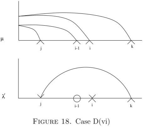
Case D. Inxµ both vertices i−1 andiare labelled by ∧. This case splits into six subcases

D(i)-(vi) as depicted in Figures 13-18. Using the same argument as in Case C, it is easy to show that in each case we have dim Homn(indλ

0

n−1Pn−1(µ), Ln(λ0)) = 1. Note that in all

cases the verticesi andj inλ0 must be in the same chamber otherwisexµ wouldn’t have the

required cap diagram. We have that cases D(i)(iii)-(v) correspond to all verticesj satisfying (11), and Cases D(ii) and (vi) correspond to all vertices j satisfying (12).

i i-1 j

i i-1 j

µ

λ

Figure 13. Case D(i)

i i-1 j

i

λ µ

j i-1

Figure 14. Case D(ii)

Finally, using the fact that all simple modules are self-dual, the restriction must have the

i i-1

j k

i i-1

j k

µ

λ

Figure 15. Case D(iii)

i-1 i j

k

i i-1

λ µ

k j

Figure 16. Case D(iv)

i k

i-1 j

k i

λ µ

j _i-1

i k i-1

j

k i

λ µ

j i-1

Figure 18. Case D(vi)

Corollary 4.0.5. Let λ∈Aδ. Then the dimension of Ln(λ) is given by the number of walks

on Yδ from ∅ to λ.

Proof. This follows immediately by induction onn using Propositions 4.0.1 and 4.0.2.

5. Walk bases for simple modules

5.1. Leduc-Ram walk bases for generic simple modules. In this section we recall the construction given in [11] of walk bases for simple modules for the generic Brauer algebra

Bn(u), whereuis an indeterminate and the algebra is defined over_C(u). Their construction uses two combinatorial objects associated with partitions which we now recall. We start with the King polynomials, which were originally derived from Weyl’s character formula in [7].

Let λ be a partition, and denote by [λ] its Young diagram. For each box (i, j) ∈ [λ] we define

d(i, j) =

λi+λj −i−j+ 1 if i≤j

−λT

i −λTj +i+j−1 if i > j

We also write h(i, j) for the usual hook length. We then define the King polynomial

Pλ(u) =

Y

(i,j)∈[λ]

u−1 +d(i, j)

h(i, j) .

For example, P∅(u) = 1, P(1)(u) = u,

P(12₎(u) =

u(u−1)

2 , P(2)(u) =

(u+ 2)(u−1)

2 ,

P(13₎(u) =

u(u−2)(u−1)

3! , P(2,1)(u) =

(u+ 2)u(u−2)

3 , P(3)(u) =

(u+ 4)u(u−1)

3! ,

P(14₎(u) =

u(u−3)(u−2)(u−1)

4! , P(2,12)(u) =

We denote the set of all walks on the Young graph Y by Ω and the subset of all walks of length n starting at ∅ and ending at λ by Ωn_{(λ). For a walk S ∈ Ω, we write S =}

(s(0), s(1), s(2), ...) where s(m) is the m-th partition in the walk S. We then define Ωm(S)

to be the set of all walks T that differs fromS in at most position m, that is t(j) =s(j) for all j 6=m. If T ∈ Ωm(S) we say that (S, T) form an m-diamond pair, and in this case we

define the Brauer diamond3m(S, T)∈Z[u] by

3m(S, T) =

          

±(s(m+ 1)k−k−t(m)l+l)

if t(m) =s(m−1)±l

and s(m+ 1) =s(m)±k

±(u+t(m)l−l+s(m+ 1)k−k)

if t(m) =s(m−1)∓l

and s(m+ 1) =s(m)±k

Theorem 5.1.1. [11](6.22) There is an action of the generic Brauer algebra Bn(u) on the

C(u)-vector spaceΠλ with basis Ωn(λ) given by

σmT =

X

S∈Ωm(T)

(σm(u))STS

emT =

X

S∈Ωm(T)

(em(u))STS

where

(σm(u))SS =

( 1

3m(S,S) if s(m−1)6=s(m+ 1)

1

3m(S,S)

1− Ps(m)(u) Ps(m−1)(u)

otherwise

and for S 6=T

(σm(u))ST =

     q

(3m(S,S)−1)(3m(S,S)+1)

3m(S,S)2 if s(m−1)6=s(m+ 1)

− 1

3m(S,T)

√

Ps(m)(u)Pt(m)(u) Ps(m−1)(u)

otherwise ,

and similarly for any S, T

(em(u))ST =

( √_P

s(m)(u)Pt(m)(u)

Ps(m−1)(u) if s(m−1) =s(m+ 1)

0 otherwise

We will give a geometric interpretation of the King polynomials Pλ(u) and the Brauer

diamonds 3m(S, T) in the next two sections. This will allow us to define an action of the

Brauer algebra Bn(δ) on the C- span of all δ-restricted walks in Ωn(λ).

5.2. A geometric interpretation of the roots of the King polynomials. Recall the definition of the δ-degree of singularity of a partition given in Definition 2.4.1.

Theorem 5.2.1. Fix δ ∈ _Z and let λ ∈ Λ. Let mδ(λ) be the multiplicity of δ as a root of

the King polynomial Pλ(u). Then we have

mδ(λ) = degδ(λ)−degδ(∅).

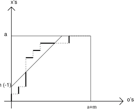
Proof. Writea = min{#(◦’s in xλ),#(×’s in xλ)}and letδ = 2mor 2m+ 1 for somem∈Z.

Using Example 3.1.1 and Lemma 3.2.2 we have that for m ≥0,

a = #(×’s in xλ) = deg_δ(λ) = deg_δ(λ)−deg_δ(∅)

as deg_δ(∅) = 0; and for m <0 we have

a = #(◦’s in xλ)

= #(◦’s in xλ)−#(×’s in xλ) + #(×’s in xλ)

= m+ #(×’s in xλ)

= #(×’s in xλ)−#(×’s in x∅)

= deg_δ(λ)−deg_δ(∅).

Thus it’s enough to show that mδ(λ) =a.

Now by definition ofPλ(u) and Proposition 3.2.3 we have thatmδ(λ) is precisely the number

of ×’s inxλ satisfying (5) added to the number of ◦’s in xλ satisfying (6). We can represent

the sequence of×’s and◦’s appearing in xλ reading from left to right by a graph as follows.

Start at (0,0) and for each term in the sequence add (1,0) if it is a ◦, or add (0,1) if it is a

×. The graph is given in Figure 19 for m≥0 and in Figure 20 for m <0.

a

m (-1)

a+m

o’s x’s

Figure 19. Graph representing the sequence of ×and ◦in xλ for m≥0

Now observe that the admissibility conditions (5) and (6) can be rephrased as follows. A

× (resp. ◦) satisfies (5) (resp. (6)) if and only if the corresponding step in the graph is below (resp. above) the line y=x+m−δδ,2m. Admissible (resp. non-admissible) steps are

represented by solid lines (resp. dotted lines) in the graphs. It follows immediately that the total number of admissible ×’s and ◦’s is equal to a.

Remark 5.2.2. It was shown in [17, Corollary (3.5)] that λ ∈ Aδ if and only if Pµ(δ) 6= 0

a-m

o’s x’s

a m (-1)

Figure 20. Graph representing the sequence of × and ◦ inxλ for m <0

5.3. A geometric interpretation of the Brauer diamonds. In this section we give a geometric interpretation of the Brauer diamonds when we specialise u=δ.

Recall the isomorphism between the Young graphY andZ+(ρδ) given in Section 2.2. Using

this we will view walks on Y as walks in Z+(ρδ) where each edge is of the form x→ x±i

for some x∈_RN _{and some i≥1.}

Let (S, T) be an m-diamond pair. The Brauer diamond only depends on the m −1,

m and m + 1 steps in the walks, so we will write S = (x(m− 1), x(m), x(m + 1)) and

T = (x(m−1), y(m), x(m+ 1)), where the x(i)’s andy(i)’s are in _RN_.

Theorem 5.3.1. The Brauer diamonds satisfy the following identities. Case 1. If S= (x, x±i, x±i±j), T = (x, x±j, x±i±j),

then we have for i6=j

3(S, T) = 3(T, S) = 0

3(S, S) = −3(T, T) = hx, i−ji,

and for i=j we have

3(S, S) =−1.

Case 2. If S= (x, x±i, x±i∓j), T = (x, x∓j, x±i∓j) with i6=j, then we have

3(S, T) = 3(T, S) = 0

3(S, S) =−3(T, T) = ±hx, i+ji.

Case 3. If S= (x, x+α, x), T = (x, x+β, x) with α, β ∈ {±i : i≥1},

then we have

3(S, T) =3(T, S) = hx, α+βi+ 1

iin the Young diagram (that isλk+ 1 =i) and the boxlis added in column j in the Young

diagram (that is (λ+k)l+ 1 =j). Note that for S =6 T we must have k 6=l and i6=j. In

this case we have

3(S, T) = (λl+ 1)−l−(λl+ 1) +l= 0,

3(T, S) = (λk+ 1)−k−(λk+ 1) +k = 0 and

3(S, S) = (λl+ 1)−l−(λk+ 1) +k

= j−(λ0_j−1)−i+ (λ0_i−1)

= (λ0_i− δ

2 −i+ 1)−(λ

0

j − δ

2 −j+ 1) = heδ(λ), i−ji

= −3(T, T).

If i=j, then l =k+ 1 and we have

3(S, S) = (λk+1+ 1)−(k+ 1)−(λk+ 1) +k =−1.

Finally, if k =l then j =i+ 1 and we have

3(S, S) = (λk+ 2)−k−(λk+ 1) +k

= 1

= (λ0_i− δ

2 −i+ 1)−(λ

0

i+1−

δ

2−(i+ 1) + 1) = heδ(λ), i−i+1i.

5.4. Walk bases for δ-restricted simple modules. Recall the definition of the set of

δ-restricted partitions Aδ and the δ-restricted Young graph Yδ given in Section 2.2.

Note that the matrix entries defining the representation Πλ of Bn(u) given in Theorem 5.1.1 do not in general specialise to u = δ. However we will show that, for any λ ∈ Aδ, if

we only consider the submatrices with entries labelled by δ-restricted walks, then these do specialise to give a representation of Bn(δ) which is isomorphic to Ln(λ). (Note that these

do not correspond to quotients or submodules for Bn(u).)

We start by giving an explicit description of Aδ.

Proposition 5.4.1. A partitionλ belongs toAδ if and only if one of the following conditions

holds.

(i) δ≥0 and λT

1 +λT2 ≤δ.

(ii) δ =−2m (for some m∈_N) and λ1 ≤m.

(i,j)_ (i,j)

i j

x h

T

S

Figure 21. Case 1: S = (x, x+i, x+i +j), T = (x, x+j, x+i +j)

with i < j and h = hx, i −ji. Projection of RN onto the ij-plane, showing

the reflection hyperplane. Fibres containing partitions are shaded.

Proof. Forδ = 2mor 2m+ 1, the weight diagramx∅ consists ofm◦’s (form≥0) orm×for

m <0 followed by infinitely many ∨’s (see Figure 3). Moreover, all possible configurations of translation equivalent weight diagrams are given in Lemma 3.2.1 (i)-(v). It follows that the weight diagrams corresponding to partitions in Aδ are precisely those having m ◦ (for

m≥0) orm ×(for m <0) and with the other vertices either all labelled by∨’s, or labelled by one ∧ and infinitely many ∨’s, in that order. The result then follows from the end of

Section 2.2 (see Figure 4 and 5).

Remark 5.4.2. Proposition 5.4.1 also follows by combining [17] (definition before Theorem (3.4) and Corollary (3.5)(b)) with Theorem 5.2.1.

Theorem 5.4.3. [15, Theorem 2.4(b)]Let λ∈Aδ. Then there is an action of Bn(δ) on the

vector space spanned by all walks of length n on Yδ from ∅ to λ. This module is isomorphic

to Ln(λ).

Proof. We consider the action of the generic Brauer algebra Bn(u) on the Leduc-Ram

rep-resentations Πλ _{and claim that the truncation of this action to δ-restricted walks gives a}

well-defined representation by setting u=δ. It suffices to show that:

(A) all matrix entries (σm(u))ST,(em(u))ST where at least one of S or T are δ-restricted

walks do not have a pole at u=δ,

(B) the matrix entries (σm(δ))ST,(em(δ))ST, where precisely one ofSorT isδ-restricted and

the other is not, vanish.

(i,j)_ (i,j)

i j

x S

T

g

Figure 22. Case 2: S = (x, x+i, x+i−j), T = (x, x−j, x+i−j)

with i < j and g =hx, i+ji

T satisfy the relations (R1)–(R9):

(R1)σ2

i = 1

(R2)eiσi =σiei =ei

(R3)e2

i =δei

 



for all 1≤i≤n−1,

(R4)σiσj =σjσi

(R5)eiσj =σjei

(R6)eiej =ejei

 



for all 1≤i, j ≤n−1 with |i−j| ≥2,

(R7)σiσjσi =σjσiσj

(R8)σjeiσj =σiejσi

(R9)σjσiej =eiej

 



for all 1≤i, j ≤n−1 with|i−j|= 1

(which relations are known to defineBn(δ)).

We start by proving (A) and (B).

Note that if (σm(u))ST or (em(u))ST are non-zero, then (S, T) is an m-diamond pair. So

we will consider the three cases of m-diamond pairs given in Theorem 5.3.1.

Case 1. S = (x, x±i, x±i±j), T = (x, x±j, x±i±j).

First note that the submatrix of (em(u)) mixing between S and T is identically zero as s(m−1)6=s(m+ 1). So there is nothing to check here.

For i = j we have S = T and (σm(δ))SS = −1. For i 6= j, write h = hx, i −ji. As x

(i,j)_ (i,j)

i j

x _S T

Figure 23. Case 3: S = (x, x+i, x), T = (x, x+j, x) withi < j.

between the walks S and T given by

1

h

√

h2₋₁

|h| √

h2₋₁

|h| −

1

h

!

is always well-defined, see Figure 21. This proves (A).

Observe that in this case T is δ-restricted if and only if S is δ-restricted (see Figure 21). Indeed, ifSwas notδ-restricted, thenhx±i, i+kiwould be zero for somek. But asx±i±j

isδ-regular, we must havek =j. But then we would havehx±j, i+ji=hx±i, i+ji= 0

which contradicts the fact that T is δ-restricted. So there is noting to check for (B) in this case.

Case 2. S = (x, x±i, x±i∓j), T = (x, x∓j, x±i∓j) with i6=j.

As in Case 1, we have that the submatrix of (em(u)) is identically zero in this case. Write g =hx, i+ji. Then the submatrix of (σm(δ)) mixing between the walks S and T is given

by





±1

g √

g2₋₁

|g|

√ g2₋₁

|g| ∓

1

g



,

(see Figure 22). Now we claim that ifT is δ-restricted, then we cannot have g = 0. Indeed, forT δ-restricted, we have thatx,x∓j andx∓j±iall have the same degree of singularity.

Now if g = hx, i+ji = 0 then we have xj = −xi. But then, (x∓j)j = −xi ∓1 and as x∓j has the same degree of singularity asxwe must have thatx∓j has a coordinate equal

(i,j)_ (i,j) i j x T S

Figure 24. Case 3: S = (x, x+i, x), T = (x, x−j, x) with i < j.

is not strictly decreasing, which is a contradiction. Hence we have shown that g cannot be zero and the matrix entries are all well-defined, proving (A).

Now suppose that T isδ-restricted butS is not. So we have that xisδ-regular and x±i

is not. Thus we have that xi±1 =−xh for some h. But as x±i∓j is δ-regular, we have

that h=j and soxj =−xi∓1. This shows that g =hx, i+ji=∓1 and henceg2−1 = 0.

This proves (B).

Case 3. S = (x, x+α, x), T = (x, x+β, x) where α, β ∈ {±i : i ≥ 1}, see Figures 23

and 24. In this case the submatrix of (σm(δ)) mixing between S and T is given by



  

1 2hx,αi+1

1− Px+α(δ) Px(δ)

−1

hx,α+βi+1

√

Px+α(δ)Px+β(δ) Px(δ)

−1

hx,α+βi+1

√

Px+α(δ)Px+β(δ) Px(δ)

1 2hx,βi+1

1− Px+β(δ) Px(δ)



  

and the submatrix of (em) mixing betweenS and T is given by





|Px+α(δ)| Px+α(δ)

√

Px+α(δ)Px+β(δ) Px(δ)

√

Px+α(δ)Px+β(δ) Px(δ)

|Px+β(δ)| Px+β(δ)



.

First note that if T isδ-restricted, then using Theorem 5.2.1 we have that Px(δ)6= 0. Thus

the entries in the submatrix representing the action of em are all well-defined.

Now suppose that we had hx, α +βi + 1 = 0, that is hx, α +βi = −1. So we get

and α+β 6= 0. Moreover, as x+β is strictly decreasing we cannot have α+β =±(i−j).

Now suppose hx+β, i+ji= 0, with α =±i and β =±j. As T is δ-restricted, we have

that x and x+β =x±j have the same degree of singularity. Thus x must have an entry

equal to xi±1 (in position i±1). But then x+α=x±i is not strictly decreasing, which

is a contradiction. This proves that the off-diagonal entries of (σm) are well-defined.

Now, if T is δ-restricted but S is not then we have that the off diagonal entries in (σm)

and (em) are all zero using Theorem 5.2.1. This proves (B).

Now we claim that the diagonal entries in (σm) are also well-defined. Observe that it is

possible to have 2hx, αi+1 = 0. However we claim that, as a polynomial inδ,Px(δ)−Px+α(δ)

is divisible by 2hx, αi+ 1. To see this, note that before specialisation, the matrix (σm(u))

gives a well-defined representation ofBn(u) and so we have (σm(u))2 =I the identity matrix.

In particular we have that

X

T∈Ωm(S)

(σm(u))ST(σm(u))T S = 1.

So we have

(σm(u))2SS+

X

T∈Ωm(S) T6=S

(σm(u))2ST = 1.

Now we have seen that limu→δ(σm(u))ST for all T ∈Ωm(S) and T 6=S exist and are finite.

Thus we must have that limu→δ(σm(u))2SS exists and is finite. This means that (σm(u))SS is

a rational function with no poles at u= δ, proving our claim. This completes the proof of (A).

We now turn to (C). Note that it follows from (A) and (B) that the relations (R1)–(R6) are all satisfied. For example for the relation (R2) we have that for S, S0 any δ-restricted walks

X

T∈Ωm(S)

(em(u))ST(σm(u))T S0 =

X

V∈Ωm(S)

(σm(u))SV(em(u))V S0 = (e_m(u))_SS0.

Now note that if T (resp, V) is not δ-restricted then we know from (B) that the matrix entries specialise to 0 when setting u = δ. Thus all terms involving non δ-restricted walks will vanish in the specialisation and hence the relation above will specialise when u = δ

to give the required relation for Bn(δ). Exactly the same argument works for all the other

relations (R1)–(R6) as these involve products of at most 2 generators.

For the relations (R7)–(R9) we also need to consider sums of products of the form

X

T,U

(gm(u))ST(hm+1(u))T U(km(u))U S0 or

X

V W

(gm+1(u))SV(hm(u))V W(km+1(u))W S0

where S and S0 are δ-restricted, T ∈ Ωm(S) and U ∈ Ωm(S0) with T ∈ Ωm+1(U), V ∈

Ωm+1(S) and W ∈ Ωm+1(S0) with V ∈ Ωm(W), and gm, hm, km ∈ {σm, em}. Note that

We need to show that, under these conditions, the matrix entries (hm(u))T U and

(hm+1(u))V W, do not have a pole at u = δ. Then using (B) as above we would have that

these relations would specialise when u = δ to give the required relations, that is, all the terms involving non δ-restricted walks would vanish in the specialisation.

Using the remark above, we can assume that none ofT, U, V, W areδ-restricted. Note that ast(m) (resp. v(m+ 1)) isδ-singular but t(m+ 2) =s(m+ 2) (resp. v(m−1) =s0(m−1)) is δ-regular, we must have t(m) 6= t(m+ 2) (resp v(m −1) 6= v(m+ 1)). This implies immediately that (em+1(u))T U = (em(u))V W = 0 and so we’re done in this case. We now

turn to (σm+1(u))T U and (σm(u))V W. By the remark above, all we need to show is that

3m+1(T, T) 6= 0 and 3m(V, V) 6= 0 when we specialise to u = δ. We use Theorem 5.3.1.

Note that under our assumption Case 3 cannot happen. Moreover, in Case 1 the Brauer diamonds are independent of u and so there is nothing to prove there. In Case 2 we have

3m+1(T, T) =±ht(m), i +ji=±ht(m+ 2), i+ji 6= 0

in the specialisation, as t(m+ 2) isδ-regular. Similarly, we have

3m(V, V) =±hv(m−1), i+ji 6= 0

in the specialisation, as v(m−1) is δ-regular. So we have proved (C).

It remains to show that this module is isomorphic toLn(λ), defined as the simple head of

the standard module ∆n(λ). Denote the representation ofBn(δ) onδ-restricted walks defined

above by ˜Ln(λ). By looking at the action of the generators σm and em , we immediately see

that

resnL˜n(λ)∼=

M

λ0_{∈supp(λ)∩Aδ}

˜

Ln−1(λ0)

We will prove by induction on n that ˜Ln(λ) ∼= Ln(λ). If n = 0 then there is nothing to

prove. Assume that the result holds for n−1. Let λ0 ∈ supp(λ)∩Aδ (note that as δ 6= 0,

we have supp(λ)∩Aδ6= 0). Then we have

Homn(∆n(λ),Ln˜ (λ)) ∼= Homn(indλn−1∆n−1(λ0),Ln˜ (λ))

∼

= Homn−1(∆n−1(λ0),resλ

0

n Ln˜ (λ)) ∼

= Homn−1(∆n−1(λ0),prλ

0

⊕µ∈supp(λ)∩Aδ L˜n−1(µ)) ∼

= Homn−1(∆n−1(λ0),prλ

0

⊕µ∈supp(λ)∩Aδ Ln−1(µ)) by induction ∼

= Homn−1(∆n−1(λ0), Ln−1(λ0))

= _C.

This shows that ˜Ln(λ) contains Ln(λ) as a composition factor. But using Corollary 4.0.5,

we have that dimLn(λ) = dim ˜Ln(λ) and so we must have ˜Ln(λ)∼=Ln(λ).

References

[1] R. Brauer, On algebras which are connected with the semi-simple continuous groups, Annals of Mathe-matics 38(1937), 854-872.

[3] A. G. Cox, M. De Visscher, P. P. Martin,The blocks of the Brauer algebra in characteristic zero, Repre-sentation Theory 13(2009), 272-308.

[4] A. G. Cox, M. De Visscher, P. P. Martin,A geometric characterisation of the blocks of the Brauer algebra, J. London Math. Soc80 (2009), 471-494.

[5] A. G. Cox, M. De Visscher, P. P. Martin, Alcove geometry and a translation principle for the Brauer algebra, J. Pure Appl. Algebra215(2011), 335-367.

[6] W. F. Doran, D. B. Wales, P. J. Hanlon,On semisimplicity of the Brauer centralizer algebras, J. Algebra 211(1999), 647-685.

[7] N. El Samra, R.C. King,Dimensions of irreducible representations of the classical Lie groups, J.Phys.A: Math.Gen, Vol.12 (1979), 2317-2328.

[8] R. Hartmann and R. Paget, Young modules for Brauer algebras and filtration multiplicities, Math. Z. 254(2006), 333-357.

[9] J. E. Humphreys,Reflection groups and Coxeter groups (CUP, 1990).

[10] A. Kleshchev, Branching rules for symmetric groups and applications, in Algebraic Groups and their Representations, R.W. Carter and J. Saxl editors, NATO ASI Series C, Vol. 517, Kluwer Academic Publishers, Dordrecht/Boston/London, 1989, 103-130.

[11] R. Leduc, A. Ram, A ribbon Hopf algebra approach to the irreducible representations of centralizer algebras: The Brauer, Birman-Wenzl, and type A Iwahori-Hecke algebras, Advances in Math.125(1997), 1-94.

[12] T. Lejcyk, A graphical description of (an−1, dn) Kazhdan-Lusztig polynomials, 2010, Diplomarbeit, Bonn.

[13] R.J.Marsh, P.P.Martin,Tiling bijections between paths and Brauer diagrams, J. Algebraic combinatorics 33n.3 (2011), 427-453.

[14] P. P. Martin, The decomposition matrices of the Brauer algebra over the complex field, preprint (2009) (http://arxiv.org/abs/0908.1500), Trans. A.M.S. to appear.

[15] A. Ram and H. Wenzl,Matrix units for centralizer algebras, J. Algebra145(1992), 378-395. [16] H. Rui,A criterion on the semisimple Brauer algebras, J. Comb. Theory Ser. A111(2005), 78-88. [17] H. Wenzl,On the structure of Brauer’s centralizer algebra, Ann. Math.128(1988), 173-193.

E-mail address: M.Devisscher@city.ac.uk