Estimating spot volatility with high-frequency financial data

City, University of London Institutional Repository

Citation

: Zu, Y. and Peter Boswijk, H. (2014). Estimating spot volatility with

10.1016/j.jeconom.2014.04.001

This is the unspecified version of the paper.

This version of the publication may differ from the final published

version.

Permanent repository link:

Link to published version

: http://dx.doi.org/10.1016/j.jeconom.2014.04.001

Copyright and reuse:

City Research Online aims to make research

outputs of City, University of London available to a wider audience.

Copyright and Moral Rights remain with the author(s) and/or copyright

holders. URLs from City Research Online may be freely distributed and

linked to.

Estimating spot volatility with high-frequency

financial data

Yang Zu

City University London

H. Peter Boswijk

University of Amsterdam

February 7, 2014

Abstract

We construct a spot volatility estimator for high-frequency financial data which

contain market microstructure noise. We prove consistency and derive the

asymp-totic distribution of the estimator. A data-driven method is proposed to select the

scale parameter and the bandwidth parameter in the estimator. In Monte Carlo

simulations, we compare the finite sample performance of our estimator with some

existing estimators. Empirical examples are given to illustrate the potential

appli-cations of the estimator.

JEL Classification: C58, C13, C14.

Keywords: spot volatility, market microstructure noise, subsampling, scale selection,

bandwidth selection.

∗_{Email: Yang.Zu@city.ac.uk. Department of Economics, City University London, Northampton}

Square, EC1V 0HB, London, United Kingdom. Telephone: +44 (0)20 7040 8619. Fax: +44 (0)20 7040 8580.

†_{Email: H.P.Boswijk@uva.nl. Amsterdam School of Economics, University of Amsterdam,}

1

Introduction

Spot volatility, also known as instantaneous volatility, measures the strength of return

variations at a certain time point, expressed per unit of time (Andersen et al. (2010)).

Spot volatility has important applications in studying the intraday patterns of the

volatil-ity process, testing price jumps (Lee and Mykland (2007), Veraart (2010)), and estimating

parametric stochastic volatility models (Bandi and Reno (2009), Kanaya and Kristensen

(2010)). In this paper, we are interested in the nonparametric estimation ofspot volatility

with high-frequency financial data.

Spot volatility estimation in the literature dates back to Merton (1980), who

consid-ered a constant volatility model. Later on, researchers tended to estimate volatility in the

context of the ARCH model (Engle (1982)), the GARCH model (Bollerslev (1986)), and

their numerous variations. Nonparametric estimation of spot volatility in the context of

diffusion models was firstly considered by Foster and Nelson (1996). Andreou and

Ghy-sels (2002) conducted simulation studies using Foster and Nelson’s estimator and some

related estimators. Recent contributions include Mykland and Zhang (2008), Fan and

Wang (2008) and Kristensen (2010).

High-frequency financial data have become more accessible for academic research in

recent years. In contrast to low frequency (daily, weekly or longer sampling frequency)

financial datasets, high-frequency datasets are characterized by the large number of

obser-vations they contain and the existence of so-called market microstructure noise. O’Hara

(1998) made theoretical studies of market microstructure noise; Andersen et al. (2000)

and Hansen and Lunde (2006) analyzed the empirical characteristics of the noise.

Existing research on volatility measurement for high-frequency data focuses mainly

on the ex post nonparametric measurement of the integrated volatility of the

underly-ing efficient price process. Andersen et al. (2001) and Barndorff-Nielsen and Shephard

(2002) made important early contributions to the use ofrealized variance to estimate the integrated volatility. However, they did not consider the effects of market

microstruc-ture noise, and the realized variance estimator can only be applied to sparsely sampled

data, where the effects of noise are small. The problem of estimating integrated volatility

under noise was first studied by Zhou (1996), who gave an unbiased but inconsistent

es-timator for integrated volatility. A¨ıt-Sahalia et al. (2005) considered a constant variance

model and gave a Maximum Likelihood Estimator for the constant variance. Later, four

types of estimators were proposed for estimating integrated volatility in the presence of

noise. These are the subsampling-based Two Scale Realized Variance (TSRV) estimator

by Zhang et al. (2005) and the Multiscale Realized Variance (MSRV) estimator by Zhang (2006); the Realized Kernel (RK) estimator by Barndorff-Nielsen et al. (2008), which is

based on Zhou (1996)’s first order moving average correction; the pre-averaging method

Likeli-hood Estimator (QMLE) by Xiu (2010), which is based on the estimator in A¨ıt-Sahalia

et al. (2005).

In this paper, we study the problem of estimating spot volatility with high-frequency

data and we explicitly consider the effects of market microstructure noise. Our approach

is closely related to the literature on integrated volatility measurement with noise. We

construct our estimator based on the Two Scale Realized Variance estimator by Zhang

et al. (2005) — our estimator calculates the increment of the Two Scale Realized

Vari-ance estimator over a small interval and applies an appropriate normalization. Under

appropriate conditions, we prove consistency and derive the asymptotic distribution of

our estimator and propose a data-driven procedure to select tuning parameters. In prac-tically meaningful Monte Carlo simulations, we compare our estimator with existing

methods in terms of several error measures and we demonstrate the improved accuracy

in using our estimator.

Some recent research is closely related to this paper. Mykland and Zhang (2008)

independently proposed the same estimator as in our paper, but did not provide a

com-plete asymptotic theory. Bandi and Reno (2009), Ogawa and Sanfelici (2011), Bos et al.

(2012), among others, have considered spot volatility estimators based on the Realized

Kernel estimator and the Pre-Averaging estimator. In a concurrent paper, Mancini et al.

(2012) (Section 3.1) have proposed a two-scale estimator for spot volatility weighted by the so-called delta sequence and have provided theoretical analysis; our estimator is

a special case of their estimator with equal weights. We provide more comprehensive

asymptotic and finite sample studies for our estimator; we also study the problem of

bandwidth and scale parameters selection, which is important for practical

implemen-tation. In the presence of jumps but without noise, spot volatility has been studied by

A¨ıt-Sahalia and Jacod (2009), Ngo and Ogawa (2009) and Andersen et al. (2009). Munk

and Schmidt-Hieber (2010b) and Munk and Schmidt-Hieber (2010a) studied the best

possible convergence rate of any spot volatility estimator in a volatility model observed

with noise, where the volatility process is assumed to be a deterministic function. Hoff-mann et al. (2010) derived a minimax bound for the same problem in a genuine stochastic

volatility model observed with noise, they showed that this bound is “nearly optimal”

in their definition and they proposed a wavelet estimator that achieves this rate. Their

rate isn−1/8 _{if translated to the present context, up to some logarithmic corrections. Our}

estimator does not have the best rate of convergence in their sense, we discuss possible

extensions to improve the convergence rate in Section 6.

The structure of this paper is as follows. Section 2 introduces the setup of the problem.

Section 3 defines the estimator, studies its asymptotic properties and the problem of

bandwidth and scale selection. Section 4 conducts Monte Carlo studies on the finite-sample properties of the estimator and Section 5 contains two empirical applications to

7 concludes the paper. Proofs are collected in Appendix A and technical lemmas are

collected in Appendix B.

Throughout the paper, hX, Yi denotes the quadratic covariation of two processes X

andY;−→d denotes converge in distribution;−→st denotes stable convergence in distribution;

p

−→denotes converge in probability; for a real number x,bxcdenotes its integer part. We call σ2

t the spot variance at timet, and we call σt the spot volatility at time t. However,

as in the financial econometrics literature, when we use the termspot volatility in general

discussions, it could refer to either σ2

t orσt, depending on the context.

2

The model

Let {Xt} be a univariate log price process, assumed to be a Brownian semimartingale,

satisfying

dXt = µtdt+σtdWt, t∈[0,1],

where {Wt} is a standard Brownian motion; {µt} is the spot drift process, and {σt} is

the spot volatility process; both are predictable. We further assume:

A1 the processes {µt} and {σt} have continuous sample paths.

A2 the process {σt} is positive.

Since X is a Brownian semimartingale, it has continuous sample paths, and its quadratic variation process satisfies

hX, Xi_t= Z t

0

σ2_sds, t∈[0,1],

such that the spot volatility satisfies

σ_t2 = dhX, Xit

dt . (1)

Taking into account the market microstructure noise existing in high-frequency financial data, we further assume

A3 X is not observable, but

Yt =Xt+εt

is observed over the interval [0,1] in discrete time over a grid ti = i/n for i =

A4 {εti}

n

i=1 are independent and identically distributed (i.i.d.) with mean 0, variance

ω2_{, and with finite fourth moment. Furthermore, {ε} ti}

n

i=1 are independent of the

{Xt} process.

The continuity assumption on the volatility sample paths accommodates a large class of spot variance processes such as diffusion processes, long memory, deterministic patterns

as well as nonstationarity. The model allows for possible dependence between {Wt} and

{σt}, so leverage effects are allowed in this model.

The model specification and Assumption A1 exclude the possibility of jumps in both

the price process and the volatility process. Assumption A4 excludes the possibility

that the noise is dependent over time (so called dependent noise) and that the noise is

dependent of the efficient price process (so-called endogenous noise). We discuss possible

extensions to these cases in Section 6.

3

The estimator and its properties

3.1

The estimator

We are interested in estimating the realization of the spot variance process {σ2

t} at any

time t ∈ (0,1). Our estimator is based on the Two Scale Realized Variance estimator (TSRV) by Zhang et al. (2005).

The TSRV estimator uses a subsampled and averaged Realized Variance (RV)

esti-mator over a scale K, together with a usual Realized Variance estimator to correct the effects of noise. It is defined as

TSRV = [Y, Y]K− n¯

n[Y, Y],

where

[Y, Y]K := 1

K

n

X

i=K

(Yti −Yti−K)

2_,

[Y, Y] :=

n

X

i=1

(Yti−Yti−1) 2_,

¯

n := n−K + 1

K .

The definition of [Y, Y]K appears to be different from the original formulation in Zhang et al. (2005), but is an equivalent reformulation of their definition, which was also used

by Zhang (2006).

Our estimator is constructed using equation (1) – a theoretical time derivative is

[t−h, t], a filtering version of the estimator for the spot variance σ2

t is defined as:

b

σ2 t =

TSRVt−TSRVt−h

h . (2)

We call it a filtering version of the estimator because it only uses data up to time t. Similarly, a smoothing version of the estimator which uses both lead and lagged data at

time t could be constructed as follows:

b

σ2 t =

TSRVt+h/2−TSRVt−h/2

h .

Here we split the bandwidth evenly between leads and lags. In the following, all the

theoretical results will be stated for the filtering version of the estimator. Analogous

results apply to the smoothing version. In the Monte Carlo experiment, we study both

versions of the estimator.

We call our estimator the Two Scale Realized Spot Variance (TSRSV) estimator.

To have a direct expression for the estimator, we first introduce some notation. For a

sequence {Zti, i= 0,1, . . . , n}, define

[Z, Z]0_tK,h := 1

h

X

t−h≤ti≤t

(∆K_Z ti)

2

K =

1

h

X

t−h≤ti≤t

(Zti−Zti−K)

2

K ,

where we use the notation ∆K _{for the Kth difference operator; and we use a}0 _{to signify}

this is a numerical time derivative; when K = 1, we write [Z, Z]0h

t := [Z, Z]

0_1,h

t . Denote

ˆ

V_tK,h as the filtering version of the TSRSV estimator at time t as in (2), it is defined as:

ˆ

V_tK,h= [Y, Y]0_tK,h− n¯

n[Y, Y]

0_h

t ,

where

¯

n= nh−K+ 1

Kh .

The estimator depends on a subsampling size parameter K, which we call the scale parameter, and an interval length parameter h, which we call the bandwidth parameter.

3.2

Decomposition

To study the statistical properties of ˆV_tK,h as an estimator of σ2

t, we first make a

“bias-variance”-like decomposition for the difference of the two:

ˆ

V_tK,h−σ_t2 =

ˆ

V_tK,h− 1

h

Z t

t−h

σ_s2ds

+ 1 h Z t

t−h

σ_s2ds−σ2_t

where P0 and P1 are defined implicitly and can be viewed as the variance and the bias

part, respectively. However, note that this is not the bias-variance decomposition defined

for usual nonparametric estimators, because under our assumption of possible existence

of leverage effects, E[ ˆV_tK,h] 6= Rt t−hσ

2

sds/h. The variance part P0 is closely related to a

similar quantity studied for the TSRV estimator, and can be analogously decomposed

into two parts as in Zhang et al. (2005):

ˆ

V_tK,h− 1

h

Z t

t−h

σ_s2ds

=

[Y, Y]0_tK,h−[X, X]0_tK,h− n¯

n[Y, Y]

0_h

t

+

[X, X]0_tK,h− 1

h

Z t

t−h

σ_s2ds

:= P2+P3,

where P2 and P3 are defined implicitly. Using the terminologies in the above mentioned

paper, these are the “error due to noise” part and “error due to discretization” part,

respectively.

We study the “bias” part P1 first, for which we need make more specific assumptions

on the path properties of the volatility process. We assume:

A5 The spot variance process {σ2

t} is an Itˆo process, satisfying

dσ_t2 = Γtdt+ ΛtdBt,

where {Γt} and {Λt} are stochastic processes with continuous sample paths. {Bt}

is a standard Brownian Motion, possibly correlated with {Wt}.

This was the assumption used in Mykland and Zhang (2008) about the volatility

process. Under this assumption, the limiting distribution ofP1 can be derived:

Proposition 1 Under Assumptions A1, A2 and A5, as n → ∞, h→0, nh→ ∞,

h−1/2P1 st

−→ r

1 3Λ

2 tZ

P1_,

where ZP1 _{is a standard normal variable independent of the σ-algebra generated by the}

X process. The stable convergence is with respect to the σ-algebra generated by the X

process.

Here P1 converges to a mixed normal distribution stably, where Λt is the diffusion

parameter of the spot variance process, which is random. The rate of convergence h−1/2

is implied by the continuous semimartingale assumption we make for the spot variance

The diffusion assumption on the spot variance process is rather restrictive. To

accom-modate more classes of models for the spot variance process, we could relax Assumption

A5 to a H¨older’s type continuity assumption:

A5-1 For almost all paths of the spot variance process,

σ

2 t

(m)

− σ2_s(m)

6C|t−s|

α

, for allt, s∈[0,1],

where m _> 0 is an integer, the superscript (m) denotes the mth derivative with respect to time, and 0< α <1.

This assumption was used in Kristensen (2010). It is very general and accommodates

diffusion process, long memory stochastic differential equations (as in Comte and Renault

(1998)), deterministic patterns as well as nonstationarity in the spot variance process. In particular, continuous semimartingales are allowed for in the assumption withm= 0 and

α < 1/2 (see for example, Ch. V, Exercise 1.20 of Revuz and Yor (1998)). The L´evy’s modulus of continuity type assumption sup_|t−s|6h|σ2

t −σs2|=Op

h1/2_|logh|1/2

(e.g. in

Fan and Wang (2008)) is also included in this assumption, as well as a deterministic spot

variance function. Under A5-1, a central limit theorem for P1 is not available, but the

following upper bound can be easily derived:

Proposition 2 Under Assumptions A1, A2 and A5-1, P1 =Op(hm+α).

We then study the “due to noise” part P2 and the “due to discretization” part P3.

We show thatP2 converges to a normal distribution conditional on the X process, while

P3 converges to a mixture of normal distributions stably. The results for these quantities

will be extensions of Zhang et al. (2005)’s corresponding results for a fixed interval to our

context of shrinking intervals.

Proposition 3 Under Assumptions A1-A4, as n → ∞, h →0, nh→ ∞, K → ∞ and

K/(nh)→0,

r

K2_h

n ×P2 =

r

K2_h

n ×

[Y, Y]0_tK,h−[X, X]0_tK,h−n¯

n[Y, Y]

0_h

t

d

−→ N 0,8ω4,

where the convergence is conditional on the X process.

K/(nh)→0,

r

nh

K ×P3 =

r

nh K ×

[X, X]0_tK,h− 1

h

Z t

t−h

σ2_sds

st

−→ r

4 3σ

4 tZP3,

where ZP3 _{is a standard normal variable independent of the σ-algebra generated by the X}

process. The stable convergence above is with respect to the σ-algebra generated by the X

process.

3.3

Asymptotic properties

The consistency of the estimator follows from the results of the previous propositions.

Theorem 1 Under Assumptions A1 to A4, with either A5 or A5-1 satisfied, when n→

∞, h→0, nh→ ∞, K → ∞, K/(nh)→0 and n/(K2_h)→0,

ˆ

V_tK,h−→p σ_t2.

The asymptotic distribution of the estimator under Assumption A5 is given in the

following theorem:

Theorem 2 Under Assumptions A1 to A5, when K = cKn2/3 and h = chn−1/6, as

n→ ∞,

n1/12Vˆ_tK,h−σ_t2−→st

8ω4 1 c2

Kch

+ cK

ch

η_t2+ch 3Λ

2 t

1₂

N(0,1),

where η2

t = 4σt4/3 and cK and ch are constants.

This limiting theorem balances the order of the “bias” term P1 and the variance term

P2+P3 to achieve a convergence rate n−1/12.

Alternatively, under the H¨older type continuity Assumption A5-1, the following

lim-iting theorem can be derived:

Theorem 3 Under Assumptions A1–A4 and A5-1, when K =cKn2/3 and n1/6hq+1/2 →

0 as n → ∞,

n1/6h1/2Vˆ_tK,h−σ_t2−→st

8ω4

c2 K

+cKηt2

12

N(0,1),

where η2

t = 4σt4/3, q =m+α is the smoothness parameter, and cK is a constant.

Because the exact distribution of the “bias” part P1 is not known, the theorem

char-acterizes an undersmoothed version of the estimator, such that P1 is dominated by P2

rate of the TSRV estimator for Integrated Variance, the TSRSV estimator for spot

vari-ance loses the rate h−1/2_{. For the bias part P}

1 to be dominated, it is necessary that

n1/6_hq+1/2 _{→ 0, this implies h = o n}−1/[3(2q+1)]

, so that the loss in the convergence

rate is h−1/2 _=n1/[6(2q+1)]_{. For continuous semimartingales, where q is any number that}

satisfies 0 < q < 1/2, the loss in the rate is n1/12 _{at least, so that the convergence rate}

with the current undersmoothing bandwidth can be infinitely close to, but is always lower

thann−1/12. As compared to then−1/12 rate in Theorem 2, the loss in the rate is because of the undersmoothing bandwidth used in this theorem.

The above estimator and the limiting distributions are for the spot variance. By

continuous mapping theorem, it is easy to show that Vˆ_tK,h1/2 is a consistent estimator for the spot volatility σt. Applying the delta method, the following limiting distribution

for the spot volatility can be obtained by applying the transformationf(x) =x1/2_{. Here}

we only give the limiting distribution for the spot volatility estimator under Assumption

A5, the result under Assumption A5-1 can be obtained analogously and we omit it here.

Theorem 4 Under Assumptions A1 to A5, when K = cKn2/3 and h = chn−1/6, as

n→ ∞,

n1/12

ˆ

V_tK,h

1/2

−σt

st

−→ 1 2σt

8ω4 1 c2

Kch

+ cK

ch

η_t2+ch 3Λ

2 t

1₂

N(0,1),

where η2

t = 4σt4/3 and cK and ch are constants.

Remark 1 The asymptotic distributions can be used to construct confidence interval,

provided that consistent estimators are available for the unknown quantities in the

expres-sions of the asymptotic variances. The noise variance ω2 can be estimated consistently using the estimator in Zhang et al. (2005):

c

ω2 ₌ 1

2n

n

X

i=1

Yti−Yti−1

2

. (3)

A consistent estimator forσ_t4 can be simply obtained by taking squares on the estimator for the spot variance. However, a consistent estimator for Λ2_t is not known (to us). Heuristically, one could use the squared increment of the estimated spot variance process

to approximate it.

3.4

Scale and bandwidth selection

To use the estimators in practice, the tuning parameters K and h need be chosen be-forehand. In this section, we propose a method to choose these parameters based on the

is defined conditional on the volatility path, because practically what we are concerned

with is estimating the realized but latent spot variance path.

Define

MISEc(K, h) :=Eσ

Z 1

0

ˆ

V_tK,h−σ_t2

2

dt

,

as the conditional MISE, where Eσ _{denotes the conditional expectation with respect to}

the sigma-algebra generated by {σt}t∈[0,1]. This is a global measure for errors made on a

generic interval [0,1].

To evaluate MISEc(K, h), we make the following decomposition:

Eσ

Z 1

0

ˆ

V_tK,h−σ_t22dt

= Z 1 0 Eσ ˆ

V_tK,h−σ_t2

2 dt = Z 1 0

EσhVˆ_tK,h−σ2_ti2 +Varσ hVˆ_tK,h−σ_t2i

dt,

where Varσ denotes the conditional variance with respect to the sigma-algebra generated

by {σt}_t∈[0,1]. With this decomposition, and using the results of Theorem 2, we know

that when K = cKn2/3 and h = chn−1/6, MISE can be approximated by the following

Asymptotic MISE (AMISE):

AMISEc(K, h) := 8 n

K2_hω

4₊ K

nh

4 3

Z 1

0

σ4_tdt+ 1 3h

Z 1

0

Λ2_tdt. (4)

From minimizing AMISEc(K, h), the parameters K and h can be solved explicitly. De-note the minimizers of AMISE asK0 _{and h}0_{. From the first order conditions we obtain:}

K0 = K∗×n2/3, h0 = h∗×n−1/6,

with constants

K∗ = 12ω

4

R1

0 σ 4 tdt

!1/3

, (5)

and

h∗ = 



8

(K∗₎2ω4+ 4 3K

∗R1

0 σ 4 tdt 1

3

R1

0 Λ

2 tdt





1/2

. (6)

K∗ and h∗ are still theoretical quantities and need to be estimated. For the constant

be estimated using the Realized Quarticity estimator in Barndorff-Nielsen and Shephard

(2002) for sparsely sampled returns. Simply plugging these two consistent estimators into

(5) we get a consistent estimator for K∗.

For the constanth∗, the noise varianceω2_{and the integrated quarticity}R1 0 σ

4

tdtcan be

estimated in the same way as we discussed in the previous paragraph. For the quadratic

variation of the spot variance processhσ2_{, σ}2_i

1 =

R1

0 Λ

2

tdt, there is no established method

to estimate it. We propose a heuristic estimator for it in the next paragraph. Plugging

the estimates for all unknown quantities into (6) we get a heuristic plug-in type estimator

for h∗, for which the theoretical properties are not known; we study its behaviour using Monte Carlo experiments in the next section.

The heuristic estimator for hσ2_{, σ}2_i

1 =

R1

0 Λ

2

tdt is constructed using its definition:

we calculate the quadratic variation of a preliminarily estimated spot variance path.

The preliminary estimate of the spot variance path can be obtained using our TSRSV

estimator with heuristically (but reasonably) chosen scale and bandwidth parameters; or

it can be obtained by applying the estimator in Mykland and Zhang (2008) or Kristensen

(2010) to sparsely sampled returns (say 5-minute returns).

Remark 2 Under Assumption A5-1, only an upper bound for the “bias” part is known;

the optimal rate of the bandwidth parameter can still be determined by optimizing the corresponding upper bound for the MISE. Since P2 +P3 = Op n−1/6h−1/2

, while the

bias part P1 =Op(hq), solving forh to maximize the sum of the two upper bounds gives

h = O n−1/[3(2q+1)]

. For a stochastic volatility model, when q < 1/2, this leads to a bandwidth h = O n−1/6

. The exact optimizing bandwidth is difficult to estimate as

this is related to H¨older’s constant in Assumption 5-1, which is hard to estimate from

data. The selection of the scale parameter will be the same as in (5).

4

Simulation study

In this section, we study the finite sample properties of the estimator. A potential concern

on the practical applicability of our estimator is the convergence rate n−1/12 _{— one may}

be afraid that this rate will be too slow to be meaningful in practical sample sizes. We aim

to address this concern in the Monte Carlo experiment. We compare the finite-sample

properties of our estimator with two types of estimators: the Realized Spot Variance

(RSV) estimator in Mykland and Zhang (2008) (see also Kristensen (2010) and Fan and

Wang (2008)) and the TSRV estimator applied to intraday intervals. These estimators

4.1

Models, parameters and error measures

We use two models as our Data Generating Processes. The models and parameter values

are the same as those used in Huang and Tauchen (2005), see also Barndorff-Nielsen et al.

(2008).

The first considered model is the One Factor Stochastic Volatility (SV1F) model:

dYt = µdt+σtdWt,

σt = exp (β0+β1τt),

dτt = ατtdt+ dBt,

where corr(dWt,dBt) = ϕ, with parameter values µ= 0.03, β1 = 0.125,α =−0.025, and

ϕ=−0.3. It is imposed that β0 =β1/(2α) to ensure the restriction Eσt2 = 1, and the τ

process is assumed to initiate from its stationary distribution N(0,−1/(2α)).

The second considered model is the Two Factor Stochastic Volatility (SV2F) model,

dYt = µdt+σtdWt,

σt = sexp (β0+β1τ1t+β2τ2t),

dτ1t = α1τ1tdt+ dB1t,

dτ2t = α2τ2tdt+ (1 +φτ2t)dB2t,

where corr(dWt,dB1t) = ϕ1 and corr(dWt,dB2t) = ϕ2 with parameter values µ = 0.03,

β0 = −1.2, β1 = 0.04, β2 = 1.5, α1 = −0.0037, α2 =−1.386, φ = 0.25, ϕ1 = −0.3 and

ϕ2 =−0.3, and the function sexp(.) is defined as

sexp(x) = (

exp(x), ifx₆log(1.5); 1.5p1−log(1.5) +x2_{/log(1.5), otherwise.}

It is a usual exponential function with a polynomial function splined in at high values to

satisfy the growth condition of the differential equation system, to ensure its solution to

exist and the Euler scheme to work. The first factor process is assumed to initiate from its stationary distribution N(0,−1/(2α1)), and the second factor process is assumed to

initiate from 0.

In the simulations, time t is measured in days, and it is assumed that there are 6.5 hours in a day (stock market trading time), so in order to simulate second data, we

take step size ∆ = 1/(6.5×60×60) = 1/23400. These models and parameter values will generate σt as percentage volatility. The SV2F model will have larger variation in

volatility than the SV1F model.

combined with the two models to make 6 scenarios, we call them SV1F1, SV1F2, SV1F3

and SV2F1, SV2F2, SV2F3, respectively.

We use four measurements of error in our comparisons, which are defined as follows:

1. Mean integrated squared error (MISE)

E

Z 1

0

ˆ

σ_t2−σ_t22 dt

1/2

2. Mean integrated squared relative error (MISRE)

E

" Z 1

0

ˆ

σ_t2−σ_t2 σ2

t

2 dt

#1/2

3. Mean integrated absolute error (MIAE)

E

Z 1

0

ˆσ2_t −σ_t2dt

4. Mean integrated absolute relative error (MIARE)

E

Z 1

0

ˆ

σ2 t −σt2

σ2 t

dt

We estimate the spot variance for every second of a trading day (6.5 hours), so the

integrals above are approximated by the discretization size of 1/23400. The expectation is evaluated by the mean of 10000 Monte Carlo replications. The computations are

conducted with OxMetrics 6.20, using the default random number generator (the George

Marsaglia multiply-with-carry algorithm) with seed 20120505.

4.2

Comparison with existing methods

We compare our estimator with two existing methods of estimating spot volatility. The

first method is the nonparametric RSV estimator as in Mykland and Zhang (2008) (see

also Fan and Wang (2008) and Kristensen (2010)). This method does not assume the

existence of market microstructure noise, and it has to be applied to sparsely sampled

data. The second method is the TSRV estimator applied to intraday intervals.

4.2.1 TSRSV estimators

We implement both the filtering version and the smoothing version of the TSRSV. The

For the smoothing version of the TSRSV, the bandwidth is equally divided between lead

and lagged observations; the noise variance is estimated as in (3); the integrated quarticity

is estimated by the Realized Quarticity estimator applied to 5-minute returns — we

did not use the preaveraging estimator to estimate the integrated quarticity, to reduce

the computational burden; for the quadratic variation of the spot variance process, the

preliminary spot variance path is estimated using the Realized Spot Variance estimator

applied to 5-minute returns, with the bandwidth selected by the cross-validation method

proposed in Kristensen (2010).

4.2.2 RSV estimator

Sparse sampling is usually used in practice to reduce the effects of microstructure noise

when dealing with high-frequency financial data. Taking 5-minute returns and

treat-ing them as clean data is common practice when measurtreat-ing integrated volatility. With

sparsely sampled data, one can apply the nonparametric RSV estimator as in Mykland

and Zhang (2008), which is a flat-weighted version of the kernel estimator of Fan and

Wang (2008) and Kristensen (2010), to estimate the spot variance. We implement both

the filtering version and the smoothing version for half-minute, 1-minute and 5-minute returns. To select the bandwidth, we use the cross-validation method proposed in

Kris-tensen (2010).

4.2.3 TSRV over fixed intraday intervals

Current volatility measurement theories are well developed for the integrated variance

estimation. Besides using these estimators for one day, we can divide the one day

inter-val into pieces and use integrated variance estimators over these subinterinter-vals as well. If one could be satisfied with a spot variance estimator which is constant over those

subin-tervals, these give estimators for the spot variance. We call these piecewise-constant

spot variance estimators. The usual integrated variance estimator for a day is a special

case — one just reports one volatility measurement for a day and uses it as a (constant)

estimator for the spot variance. In this section, we use the Piecewise-Constant TSRV

(PCTSRV) estimator for comparison purpose. The difference between the PCTSRV and

the TSRSV is, the piecewise constant estimator is using non-overlapping subsamples,

while our TSRSV estimators are using rolling subsamples.

We use equal-length subintervals for the PCTSRV estimator. That is, we divide the one day interval into equal-length intervals from the beginning of the day and we leave

out the last interval when it is shorter than the subinterval length. For this estimator,

one needs to choose the length of the subintervals h, as well as the scale parameter K. Since there is no established theory which can be used for these parameters, we use the

length and the scale parameter, respectively.

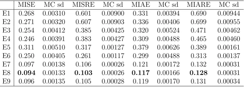
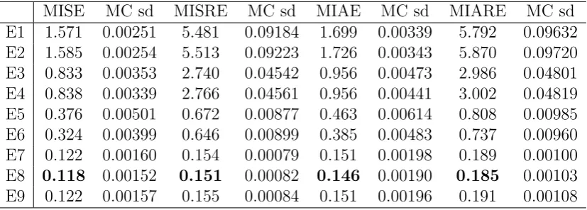
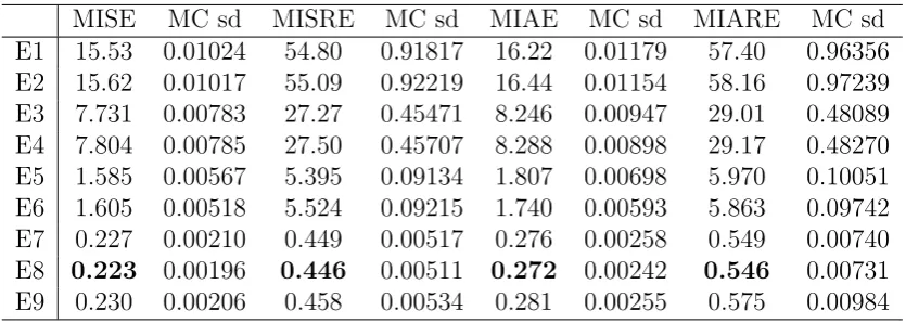
4.2.4 Monte Carlo results

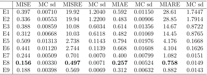
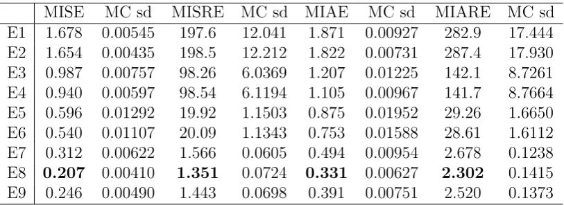
In Table 1, we give a list of the notations we used in the following tables. The Monte

Carlo evaluated error measures, together with the corresponding Monte Carlo standard

deviations are reported in Tables 2, 3, 4, 5, 6, and 7, each table corresponds to one of the

6 Monte Carlo scenarios.

We observe that all the RSV estimators are strictly dominated by TSRSV estimators in terms of all error measures. Of course we just choose 3 arbitrary sampling frequencies

for the RSV estimators in our experiment, and there may exist a sampling frequency

for these estimators to compete with our estimator. However, there is no established

theory to select the sparse sampling frequency and investigating this problem is beyond

the scope of this paper.

We also observe that the performance of the PCTSRV estimator is comparable to our

estimators. Looking further into the results, we find that in almost all scenarios and for

all error measures, the smoothing version of TSRSV gives the smallest error, with one

exception for the MISRE in SV2F3, where the filtering version of TSRSV is the best. The relative performance of the filtering version of TSRSV and the PCTSRV estimator is not

clear: for the SV1F1 scenario, the piecewise-constant estimator seems better; while for

the SV1F3 scenario, the filtering version of TSRSV is better; the evidence for the SV1F2

scenario varies for different error measures; for the 3 scenarios in the SV2F model, the

PCTSRV estimator is always better. Overall, the smoothing version of TSRSV is better

than the PCTSRV estimator, which in turn seems to be better than the filtering version

of TSRSV in more scenarios. But we remark that this comparison seems to be not fair

for the filtering version of the TSRSV estimator, as it only uses lagged observations.

[Table 1 about here.]

[Table 2 about here.]

[Table 3 about here.]

[Table 4 about here.]

[Table 5 about here.]

[Table 6 about here.]

We report the cross-validation selected bandwidths for the sparse-sampling based

method and the scale/bandwidth parameters selected by our plug-in method described

in Section 3.4. There is one set of such parameters being selected in each Monte Carlo

sample, we report the means and variances of the 10000 realizations of these parameters

in Tables 8, 9, 10, 11, 12 and 13 — each table corresponds to one of the six simulation

scenarios. We observe that as the variance of the market microstructure noise increases,

the selected scale parameter and the bandwidth parameters increase; and the SV2F model

in general induces higher scale and bandwidth parameters than the SV1F model. For

the three scenarios in the SV1F model, the selected scale parameters have mean values

8, 26 and 56 respectively; while for the three scenarios in the SV2F model the selected scale parameters have mean values 28, 39 and 57, respectively. For the three scenarios in

the SV1F model, the selected bandwidth parameters have mean values corresponding to

27 minutes, 49 minutes and 71 minutes, respectively; while for the three scenarios in the

SV2F model, the selected bandwidth parameters have mean values corresponding to 39

minutes, 60 minutes and 75 minutes, respectively.

[Table 8 about here.]

[Table 9 about here.]

[Table 10 about here.]

[Table 11 about here.]

[Table 12 about here.]

[Table 13 about here.]

5

Empirical applications

In this section, we give two empirical examples for possible applications of the TSRSV

estimator. In the first example, we use the estimator to study the intraday variation

of the volatility process. In the second example, the estimator is applied to calculating

high-frequency Value-at-Risk.

The data we use are Euro FX Futures 1-second data obtained from tickdata.com.

Euro FX Futures are currency futures contracts traded online at the Chicago Mercantile

Exchange (CME) group. The contracts are traded 23 hours a day, a usual trading day

starts from 17:00 of a day and ends at 16:00 of the next day. A trading week consists of 5 trading days, and a usual trading week starts from 17:00 on Sunday and ends at 16:00 on

5.1

Intraday variation of volatility

The spot volatility estimator can be used to study the intraday variation of volatility.

Intraday variation of volatility was previously studied mostly with parametric approaches

(e.g. Andersen and Bollerslev (1998), Taylor and Xu (1997), Boudt et al. (2011) and Bos

et al. (2012)), where it is usually assumed that there exist a periodic part in the volatility

process and one needs to take averages over many days (say, a month) to extract the periodic part. Although the existence of a periodic term in the volatility process is evident

most of the time, we remark that this assumption is questionable when the volatility

process undergoes a regime shift. Our approach is free of parametric assumptions and

we need not assume the existence of the periodic part in the volatility process, nor do

we need any specific form for it. As compared to the parametric approach of estimating

the intraday variation of volatility, our estimator performs local averages of squared

high-frequency returns around the time of interest, which we believe will better reflect the local

variation of the volatility process. Our assumption on the volatility process allows for

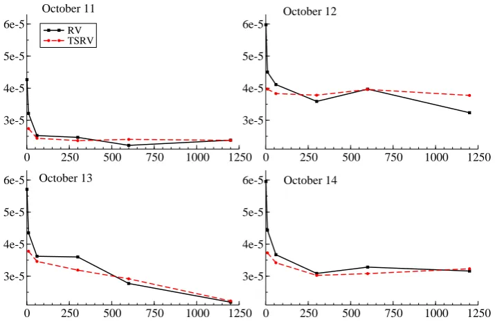
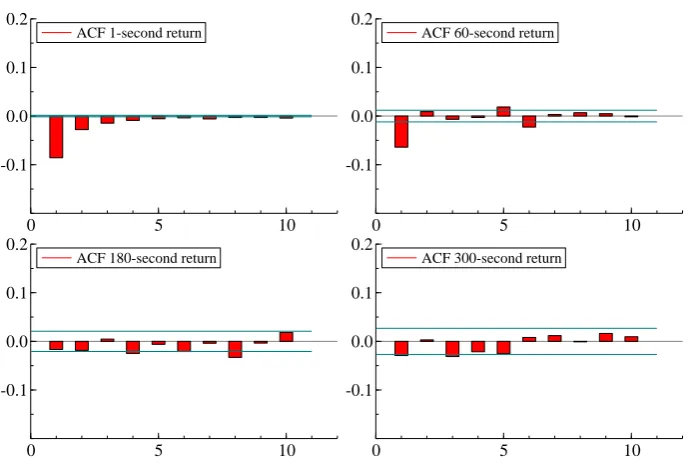
nonstationarity, structural change, periodicity and persistence in the volatility process. To illustrate the method, we choose 4 weeks of 1-second data from 11 October, 2009

to 6 November, 2009. By preliminary analysis through the volatility signature plots for

the first four days (Figure 1), and the autocorrelation function (ACF) plot (Figure 2) of

high frequency returns, we confirm the existence of market microstructure noise (from

significant first-order autocorrelation) and that the noise is dependent across time for

1-second high-frequency returns (because of non-zero higher-order autocorrelation). The

estimated noise standard deviation is around 2×10−5, which is small in magnitude as compared to the signal. From the ACF plots, we can identify that the market

microstruc-ture noise may be considered serially independent at the 1-minute frequency, and we can assume there is no noise at the 3-minute frequency.

[Figure 1 about here.]

[Figure 2 about here.]

We then apply the TSRSV and the PCTSRV estimator to the 1-minute returns, for

which we can assume i.i.d. noise; and we apply the RSV estimator to the 3-minute returns,

for which we can assume the absence of noise. We still use the cross-validation bandwidth

for the RSV estimator and we use the plug-in method to select bandwidth/scale

param-eters for the TSRSV estimator and the PCTSRV estimator. Both the RSV estimator

and the TSRSV estimator used are the smoothing version. The selected scale parameter

is two, which roughly corresponds to two-minute intervals in the current context; and

the selected bandwidth is around 0.11, which roughly corresponds to 2.5 hours for one-minute returns. The cross-validation method selects a 2 hours bandwidth for 3-one-minute

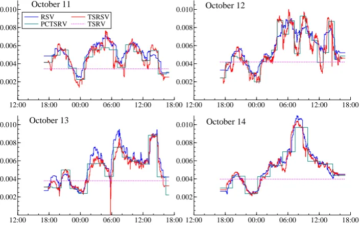
as TSRSV. To save space, we give the plots of the estimation results for the first 4 days

in Figure 3. We also give a TSRV estimate for the daily integrated variance, which is

viewed as a constant spot variance estimate for the whole day.

[Figure 3 about here.]

From the first 4 days, we can see some diurnal patterns in the spot variance. Usually

there are 4 peaks of high volatility during one day, which may correspond to the morning

and afternoon active trading hours in Asia, Europe and the US. We also note that the

differences between the Realized Spot Variance estimator and the TSRSV estimator, as

well as the piecewise constant estimator, are small. This may be due to the fact that

the magnitude of noise is small for this example. However, we still recall from the Monte Carlo evidence in the previous section that the TSRSV is more accurate than the RSV

and the PCTSRV estimator in terms of the MISE performance in most of the realistic

scenarios. We also observe that the TSRV estimator is roughly the average of the spot

variance estimators.

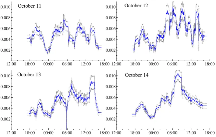
Finally, we give a plot of the estimated volatility path of a day with the 95%

(point-wise) confidence interval in Figure 4, the confidence interval is constructed by the method

described in Remark 1. Although the convergence rate of the estimator is slow, the

con-fidence intervals seem not very wide in the current example.

[Figure 4 about here.]

5.2

Intraday Value-at-Risk based on spot volatility measures

In this section, we perform a simple exercise of predicting the Value-at-Risk (VaR) of

5-minute returns to illustrate the potential use of the spot volatility estimators in financial

risk management. The dataset used here is the same as in Section 5.1.

At 5-minute level, the effect of market microstructure noise is negligible, so the

ob-served returns can be assumed to follow the model

rt=σtzt, (7)

where zt is a standard normal variable, and σt is the spot volatility. The α-VaR in

the next period is −σtΦ−1(α) for long positions and σtΦ−1(1−α) for short positions,

where Φ−1_{(.) is the quantile function of the standard normal distribution. The spot}

volatility σt can be estimated with different methods discussed earlier in this paper, for

example the TSRSV, the RSV or the TSRV estimator. The TSRV estimator is used as

a constant estimator for the spot volatility path of a whole day. Since we are performing a prediction exercise here, we include the filtering version the TSRSV estimator and the

the following, we give results by weeks to simplify the presentation. We have 20 trading

days under investigation, so we have in total 4 weeks in the dataset.

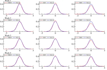
Before performing the VaR prediction, we first give density estimates of the

standard-ized returns rt/σbt. We compare the estimated density to a standard normal density; the closer to the standard normal, the better the model in (7) will provide an approximation.

We give the results in Figure 5, which contains a 4 by 3 plot. Each row is a week and

has 3 subplots which are the density estimates of 5-minute returns standardized by the

TSRSV estimator, the RSV estimator and the TSRV estimator, respectively. We observe

that the returns standardized by the TSRV is always fat-tailed, which just reflects that

the 5-minute returns are fat-tailed. The standardized returns by the TSRSV and the RSV estimator are closer to the standard normal density, this is because time-varying

volatility is able to model the fat-tailedness in data to a certain degree, if not all.

[Figure 5 about here.]

Now we perform the VaR prediction, and compare the 3 methods by the prediction

performance. We predict the 1%, 5%, 95% and 99% VaR of 5-minute returns. The

performance measure we use is the so called conditional coverage probability, which is

the empirical frequency that the failure of VaR prediction happens: for long positions, this

means that the realized return is smaller than the predicted VaR; for short positions, this means the realized return is larger than the predicted VaR. Theoretically, the conditional

coverage probability needs be the same as the theoretical level α of VaR in the left tail, and (1−α) in the right tail. In practice the frequencies will differ from the theoretical value, and the closer to the theoretical value, the more accurate is the VaR.

We give the conditional coverage probability for the left tail and the right tail of the

return distribution in Table 14 and Table 15, respectively. From the result we see that

using an intraday measure, either the TSRSV estimator or the RSV estimator, will bring

great improvement for the prediction performance as compared to the TSRV estimator.

This again justifies the necessity of spot variance estimation. The RSV seems to be always a little better than the TSRSV estimator in terms of conditional coverage probability.

However, we comment that this does not in particular mean the RSV is better than the

TSRSV: the fact that the conditional coverage probabilities are larger than the theoretical

values for both estimators means that the extreme returns in the high-frequency returns

are not well described by either method. That the RSV gives a smaller conditional

coverage probability is probably due to the fact that the RSV estimator provides a more

conservative volatility estimate than the TSRSV estimator — actually this is exactly the

case: the definition of the TSRSV estimator involves averaging the RSV over subsamples

and making a further downward correction caused by the noise. We also note that the differences between TSRSV and RSV are small, which is actually consistent with the

[Table 14 about here.]

[Table 15 about here.]

We remark that the result here does not contradict with the Monte Carlo evidence

that TSRSV is more accurate than the RSV in estimating the realized volatility path,

because there are also model uncertainties here in the VaR prediction.

6

Extensions and discussions

6.1

Multi-scale realized spot volatility estimator

In the discussion of the convergence rate after Theorem 3, we noted that the convergence

rate of the TSRV estimator is playing a role in determining the convergence rate of the

TSRSV estimator. Since the Multi-Scale Realized Variance (MSRV) estimator by Zhang

(2006) converges to the Integrated Variance at an optimal rate n−1/4_{, we conjecture that}

constructing a spot variance estimator based on the MSRV estimator will improve the

convergence rate. In this section, we discuss this issue.

Analogous to the construction of the TSRSV estimator, a filtering version of the

estimator can be constructed as:

MSRSVt =

MSRVt−MSRVt−h

h , (8)

where

MSRVt = M

X

i=1

ai[Y, Y] Ki

+ 2ωc2,

where cω2 is given as in (3) and a_i, i= 1, . . . , M are the weights satisfying

ai =

1

M2h

i M

− 1

2M2

i Mh

0

i M

,

with h(.) a continuously differentiable real-valued function satisfying

Z 1

0

h(x) dx= 0,

Z 1

0

xh(x) dx= 1.

The MSRV estimator is defined as a weighted sum of the subsampled and averaged RV

estimators over M different scales K1, K2, . . . , KM.

Using the notation defined in Section 3, the MSRSVtestimator can be written

explic-itly as

MSRSVt= M

X

i=1

ai[Y, Y]

0_K i,h

The MSRSV estimator can be decomposed as follows:

MSRSVt−σt2 = M

X

i=1

ai[Y, Y]

0_K i,h₋

σ_t2

=

M

X

i=1

ai[Y, Y]

0_K i,h₋ 1

h

Z t

t−h

σ2_sds

! + 1 h Z t

t−h

σ2_sds−σt

+ 2cω2

=

M

X

i=1

ai[X, X]

0_K i,h₋ 1

h

Z t

t−h

σ2_sds

! _M X

i=1

ai[ε, ε]

0_K i,h

+ 2ω2

!

+

M

X

i=1

ai[X, ε]

0_K i,h ! + 1 h Z t

t−h

σ_s2ds−σt

+Op n−1/2

=: A+B+C+D+Op n−1/2

,

where A, B, C, D are defined implicitly. Define the end term effects of the noise as

B2 =−

1 h M X i=1 αi i

i−1

X

j=0

ε2_tj+

nh

X

j=nh−i+1

ε2_tj

!

+ 2ω2,

and B1 :=B −B2, then the B term can be further decomposed into B1+B2. It can be

calculated that

A = Op

r

M nh

!

, B1 =Op

r

n M3_h

, B2 =Op

r 1

M h2

!

,

C = Op

r 1

M h

!

, D=Op h1/2

,

where in B, the second term comes from the end effects.

Balancing these stochastic terms we find that by taking M = O n3/5 and h =

O n−1/5, the convergence rate of the estimator can be n−1/10, which is an improvement over the TSRSV raten−1/12. We also find that takingM =O n1/2can not improve the convergence rate, as in this case, A, C and B1 are always dominated by B2. Equating

B2 with D leads to h = n−1/6 and the convergence rate of the estimator will remain at

n−1/12_.

When M =O n3/5

and h=O n−1/5

, it can be shown that

n1/10 MSRSVt−σt2

where

η2 = 4 3σ

4 t

Z 1

0

dx

Z x

0

h(y)h(x)y2(3x−y) dy+ 4 var ε2

Z 1

0

Z y

0

xh(x)h(y) dxdy+1 3Λ

2 t,

and Z is a standard normal variable. The three terms in the asymptotic variance come from A, B2 and D respectively, while B1 =Op n−3/10

and C =Op n−1/5

are smaller

order terms.

We see that by constructing an MSRSV estimator and using the same weighting

scheme as in Zhang (2006), we do get improvement in the convergence rate of the estima-tor ton−1/10_{. However, with this simple adaptation, a best convergence raten}−1/8 _{is not}

obtainable. This is due to the end term effects B2 blowing up too fast when localizing

the MSRV estimator and dominating several other terms.

Constructing a multi-scale estimator which can reach the n−1/8 _{rate is an interesting}

future research topic. Dealing with end effects will be crucial in the construction of such

an estimator.

6.2

Dependent noise

We assume i.i.d. market microstructure noise, which is not realistic from an empirical

point of view, where it is believed that the market microstructure noise is dependent over

time (see Hansen and Lunde (2006)).

When the noise is weakly dependent across time, A¨ıt-Sahalia et al. (2011) show that the classical TSRV estimator is no longer consistent for the integrated variance, they

proposed an adjusted TSRV estimator, which is robust to the dependent noise and is

consistent for the integrated variance. Intuitively, in the two-scale scheme correction for

noise, the fast scale 1 is replaced by a slower scale J, by letting J, K both converge to ∞, a consistent estimator for IV is obtained.

Based on their TSRV estimator, the following TSRSV estimator can be defined:

ˆ

V_tK,J,h= [Y, Y]0_tK,h− n¯K ¯

nJ

[Y, Y]0_tJ,h,

where ¯ni := (nh−i+ 1)/(ih), where i = K, J. We conjecture that this estimator is

robust to dependent noise.

On the other hand, since the MSRV estimator is robust to dependent noise (

A¨ıt-Sahalia et al. (2011)), we conjecture that the MSRSV estimator we defined in the previous

6.3

Endogenous noise

The market microstructure noise is assumed to be exogenous and homoscedastic in this

paper. From Hansen and Lunde (2006) however, the empirical market microstructure

noise seems to be endogenous and heteroscedastic. In the existing literature for

esti-mating integrated variance, there is no treatment for general form of endogenous and

heteroscedastic noise. Usually estimators are tuned to be robust to a certain specific type of endogeneity and heteroscedasticity. For example, Kalnina and Linton (2008)’s

jitterred TSRV is robust to the following model for the market microstructure noise:

uti = vti +εti,

vti = δγn Wti−Wti−1

,

εti = m(ti) +n

−α/2_ω(t i)ti,

where the noise{uti}is both endogenous and heteroscedastic. They impose the restriction

that α ∈ [0,1/2] and γ2 n = n1

−α_{, such that the variance of the noise {u}

ti} converges to

0 as n → ∞, which they call a small noise assumption. Barndorff-Nielsen et al. (2008)’s realized kernel estimator is robust to the following linear model of endogeneity

uti =

¯ H

X

h=0

βh Yti −Yti−1

+ ¯Uti,

where βh’s are constants, ¯U is independent of the Y process, and ¯U is a white noise

process. It can be expected that by defining a spot volatility estimator based on the jittered TSRV, the endogeneity and heteroscedasticity of the specific form can be allowed.

In the context of spot volatility estimation, Ogawa and Sanfelici (2011) proposed a

two-step regularized spot volatility estimator. Their estimator converges in the first

absolute moment under a general form of endogeneity, however it is not clear if the

robustness will be preserved if the convergence in distribution results are needed as in

this paper.

6.4

Jumps

If there is a finite activity jump component in the volatility process {σ2

t}, the theories

developed in Section 3 are only valid at the points of continuity. For discontinuous points,

we introduce the following two estimators:

TSRSVt,+ =

TSRVt−TSRVt+h

h ,

TSRSVt,− =

TSRVt−TSRVt−h

The notations are self-explanatory as the two estimators use data after the time t and before the time t, respectively. The two estimators are both consistent at continuity points. Now, let τ to be a jump point with jump size J τ, it should hold that

TSRSVτ,+ p

−→ σ_τ2+Jτ.

TSRSVτ,−

p

−→ σ_τ2.

By comparing the spot volatility estimators for a certain time point using data before and

after the point, a jump in the volatility process is identified if the difference is big, and the

jump size can be estimated by the difference of the two estimators. Gijbels et al. (2007)

and Kristensen (2010) proposed a strategy to deal with jump points. Their estimator is defined based on a so-called Residual Sum of Squares (RSS) of a local linear estimator,

however, the RSS is not directly available for the model in this paper, as the objective

function {σ2

t} to be estimated is not observable. Adapting their strategy to our model

will be an interesting extension.

Jumps in the log price process is difficult to deal with using the subsampling estimator.

However, for practical purposes, by sampling sparsely, say at the 5-minute interval, one

could use the estimator as defined in Equation (21) in Kristensen (2010), which is robust

to jumps in the price process.

7

Conclusion

Motivated by the Two Scale Realized Variance estimator and the definition of spot

vari-ance, this paper develops a nonparametric estimator for spot variance with high-frequency

financial data, which are contaminated by the market microstructure noise. Consistency

of the estimator is shown, and different asymptotic distributions are derived. In

particu-lar, this paper proposes a data-driven plug-in method to select the scale and bandwidth

parameters. In financially realistic scenarios, we conduct Monte Carlo experiments to

study the finite sample properties of our estimator. Our estimator is applied to two empirical examples. Possible extensions of the model and the estimator are discussed.

Acknowledgment

The authors wish to thank the co-editor Yacine A¨ıt-Sahalia and two anonymous referees

for helpful comments, which greatly improved the paper. They also wish to thank Peter

Hansen, Shin Kanaya, Bas Klein, Dennis Kristensen, Per Mykland, Roel Oomen, Neil

Shephard, Kevin Sheppard, Georg Strasser, Aad van der Vaart, Bert van Es, Almut Ve-raart, Lan Zhang, and seminar and conference participants at the Tinbergen Institute,

Econo-metrics, the 64th European Meeting of the Econometric Society, the 20th EC2 conference

on Real Time Econometrics, and the Oxford-Man Institute of Quantitative Finance for

helpful comments, discussions and suggestions. All remaining errors are our own. Part

of the research was conducted while Yang Zu was visiting the Oxford-Man Institute of

Quantitative Finance supported by a C. Willems Stichting travel grant; the institute’s

References

A¨ıt-Sahalia, Y. and J. Jacod (2009). Testing for jumps in a discretely observed process.

Annals of Statistics 37, 184–222.

A¨ıt-Sahalia, Y., P. Mykland, and L. Zhang (2011). Ultra high frequency volatility

esti-mation with dependent microstructure noise. Journal of Econometrics 160, 160–175.

A¨ıt-Sahalia, Y., P. A. Mykland, and L. Zhang (2005). How often to sample a

continuous-time process in the presence of market microstructure noise. Review of Financial

Studies 18, 351–416.

Andersen, T. G. and T. Bollerslev (1998). Answering the skeptics: Yes, standard volatility

models do provide accurate forecasts. International Economic Review 39, 885–905.

Andersen, T. G., T. Bollerslev, and F. X. Diebold (2010). Parametric and

nonparamet-ric volatility measurement. In Y. A¨ıt-Sahalia and L. P. Hansen (Eds.), Handbook of

Financial Econometrics, Volume 1, pp. 67–137. Amsterdam: North Holland.

Andersen, T. G., T. Bollerslev, F. X. Diebold, and P. Labys (2000). Great realizations.

Risk 13, 105–108.

Andersen, T. G., T. Bollerslev, F. X. Diebold, and P. Labys (2001). The distribution of realized exchange rate volatility. Journal of the American Statistical Association 96,

42–55.

Andersen, T. G., D. Dobrev, and E. Schaumburg (2009). Duration-based volatility

esti-mation. Global COE Hi-Stat Discussion Paper Series gd08-034, Institute of Economic

Research, Hitotsubashi University.

Andreou, E. and E. Ghysels (2002). Rolling-sample volatility estimators: Some new

theoretical, simulation, and empirical results. Journal of Business & Economic

Statis-tics 20, 363–76.

Bandi, F. M. and R. Reno (2009). Nonparametric stochastic volatility. Global COE

Hi-Stat Discussion Paper Series gd08-035, Institute of Economic Research, Hitotsubashi University.

Barndorff-Nielsen, O. E., P. R. Hansen, A. Lunde, and N. Shephard (2008). Designing

realised kernels to measure the ex-post variation of equity prices in the presence of

noise. Econometrica 76, 1481–1536.

Barndorff-Nielsen, O. E. and N. Shephard (2002). Econometric analysis of realized

volatil-ity and its use in estimating stochastic volatilvolatil-ity models.Journal of the Royal Statistical

Society Series B 64, 253–280.

Bollerslev, T. (1986). Generalized autoregressive conditional heteroskedasticity. Journal

of Econometrics 31, 307–327.

Bos, C. S., P. Janus, and S. J. Koopman (2012). Spot variance path estimation and

its application to high-frequency jump testing. Journal of Financial Econometrics 10,

Boudt, K., C. Croux, and S. Laurent (2011). Robust estimation of intraweek periodicity

in volatility and jump detection. Journal of Empirical Finance 18, 353–367.

Comte, F. and E. Renault (1998). Long memory in continuous-time stochastic volatility

models. Mathematical Finance 8, 291–323.

Engle, R. F. (1982). Autoregressive conditional heteroscedasticity with estimates of the

variance of United Kingdom inflation. Econometrica 50, 987–1007.

Fan, J. and Y. Wang (2008). Spot volatility estimation for high-frequency data. Statistics

and Its Interface 1, 279–288.

Foster, D. P. and D. B. Nelson (1996). Continuous record asymptotics for rolling sample

variance estimators. Econometrica 64, 139–74.

Gijbels, I., A. Lambert, and P. Qiu (2007). Jump-preserving regression and smoothing

using local linear fitting: a compromise. Annals of the Institute of Statistical

Mathe-matics 59, 235–272.

Hall, P. and C. C. Heyde (1980). Martingale Limit Theory and Its Application. New

York: Academic Press.

Hansen, P. R. and A. Lunde (2006). Realized variance and market microstructure noise.

Journal of Business & Economic Statistics 24, 127–161.

Hoffmann, M., A. Munk, and J. Schmidt-Hieber (2010). Nonparametric estimation of

the volatility under microstructure noise: wavelet adaptation. Preprint. Available at

arXiv 1007.

Huang, X. and G. Tauchen (2005). The relative contribution of jumps to total price

variance. Journal of Financial Econometrics 3, 456.

Jacod, J. (1997). On continuous conditional Gaussian martingales and stable convergence

in law. In J. Az´ema, M. Yor, and M. ´Emery (Eds.), S´eminaire de Probabilit´es XXXI,

pp. 232–246. Berlin: Springer.

Jacod, J., Y. Li, P. Mykland, M. Podolskij, and M. Vetter (2009). Microstructure noise

in the continuous case: the pre-averaging approach. Stochastic Processes and their

Applications 119, 2249–2276.

Kalnina, I. and O. Linton (2008). Estimating quadratic variation consistently in the

presence of endogenous and diurnal measurement error. Journal of Econometrics 147,

47–59.

Kanaya, S. and D. Kristensen (2010). Estimation of stochastic volatility models by

nonparametric filtering. CREATES Research Papers 2010-67, School of Economics

and Management, University of Aarhus.

Kristensen, D. (2010). Nonparametric filtering of the realized spot volatility: A

kernel-based approach. Econometric Theory 26, 60–93.

Lee, S. S. and P. A. Mykland (2007). Jumps in financial markets: A new nonparametric test and jump dynamics. Review of Financial Studies 21, 2535–2563.

sequences. DiMaD Working Papers 2012-10, Dipartimento di Matematica per le

Deci-sioni, Universit`a degli Studi di Firenze.

Merton, R. C. (1980). On estimating the expected return on the market: An exploratory

investigation. Journal of Financial Economics 8, 323–361.

Munk, A. and J. Schmidt-Hieber (2010a). Lower bounds for volatility estimation in

microstructure noise models. Borrowing Strength: Theory Powering Applications-A

Festschrift for Lawrence D. Brown, IMS Collection 6, 43–55.

Munk, A. and J. Schmidt-Hieber (2010b). Nonparametric estimation of the volatility

function in a high-frequency model corrupted by noise. Electronic Journal of

Statis-tics 4, 781–821.

Mykland, P. A. and L. Zhang (2008). Inference for volatility-type objects and implications

for hedging. Statistics and Its interface 1, 255–278.

Ngo, H.-L. and S. Ogawa (2009). A central limit theorem for the functional estimation

of the spot volatility. Monte Carlo Methods and Applications 15, 353–380.

Ogawa, S. and S. Sanfelici (2011). An improved two-step regularization scheme for spot

volatility estimation. Economic Notes 40, 107–134.

O’Hara, M. (1998). Market Microstructure Theory. New York: Wiley.

Podolskij, M. and M. Vetter (2009). Estimation of volatility functionals in the

simulta-neous presence of microstructure noise and jumps. Bernoulli 15, 634–658.

Podolskij, M. and M. Vetter (2010). Understanding limit theorems for semimartingales:

a short survey. Statistica Neerlandica 64, 329–351.

Revuz, D. and M. Yor (1998). Continuous Martingales and Brownian Motion (3rd ed.).

Berlin: Springer.

Taylor, S. J. and X. Xu (1997). The incremental volatility information in one million

foreign exchange quotations. Journal of Empirical Finance 4, 317–340.

Veraart, A. (2010). Inference for the jump part of quadratic variation of Itˆo

semimartin-gales. Econometric Theory 26, 331–368.

Xiu, D. (2010). Quasi-maximum likelihood estimation of volatility with high frequency data. Journal of Econometrics 159, 235–250.

Zhang, L. (2006). Efficient estimation of stochastic volatility using noisy observations: a

multi-scale approach. Bernoulli 12, 1019–1043.

Zhang, L., P. A. Mykland, and Y. A¨ıt-Sahalia (2005). A tale of two time scales:

Deter-mining integrated volatility with noisy high-frequency data. Journal of the American

Statistical Association 100, 1394–1411.

Zhou, B. (1996). High-frequency data and volatility in foreign-exchange rates. Journal

Appendix A: Proofs

Proof (of Proposition 1) This is essentially part (c) of Theorem 1 of Mykland and Zhang

(2008).

P1 =

1

h

Z t

t−h

σ_s2ds−σ2_t

= 1

h

Z t

t−h

σ_s2−σ_t2ds

= 1

h σ

2 s −σ

2 t

|t

t−h−

1

h

Z t

t−h

sdσ_s2

= 1

h

Z t

t−h

[(t−h)−s] dσ2_s

= 1

h

Z t

t−h

[(t−h)−s] Γsds+

1

h

Z t

t−h

[(t−h)−s] ΛsdBs.

where in the third equality integration by parts is used, and in the last equality

Assump-tion A5 is used. For the first term,

1

h

Z t

t−h

[(t−h)−s] Γsds =

1

h

Z t

t−h

[(t−h)−s] ds(Γt+Op(h))

= −1

2h(Γt+Op(h)) = Op(h).

For the second term, note that _h1Rt

t−h[(t−h)−s] ΛsdBs is an increment of a

martin-gale _h1Rt

0 [(t−h)−s] ΛsdBs, and we will use Theorem A.2 of Mykland and Zhang (2008)

to derive its asymptotic properties. To calculate the increment of the quadratic variation

process, we first calculate the quadratic variation process of 1_hR₀t[(t−h)−s] ΛsdBsitself,

first denote Mt= 1_h

Rt

0 [(t−h)−s] ΛsdBs, so that

hM, Mi_{(s−(t−h))h+(t−h)}− hM, Mi_t−h = 1

h2

Z t−h+(s−(t−h))h

(t−h)

[(t−h)−u]2Λ2_udu

= 1

h2

Z t−h+(s−(t−h))h

(t−h)

[(t−h)−u]2du Λ2_t−h+Op(h)

= 1

h2 ×

1

3[u−(t−h)]

3

|t_t−−h_h+(s−(t−h))h Λ2_t−h+Op(h)

= 1

h2 ×

1

3(s−(t−h))

3

h3 Λ2_t−h+Op(h)

= 1

3h×(s−t+h)

3

Λ2_t−h+Op(h)