A combined rh-adaptive scheme based on domain subdivision - Formulation and linear examples

A combined

rh

-adaptive scheme based on domain subdivision.

Formulation and linear examples

Harm Askes

_{and Antonio Rodrguez-Ferran}

1_{Faculty of Civil Engineering and Geosciences;Koiter Institute Delft=Delft University of Technology;}

P.O. Box 5048;2600 GA Delft;The Netherlands

2_{Departament de MatemÂatica Aplicada III;Universitat PolitÂecnica de Catalunya;E.T.S. d’Enginyers de}

Camins;Canals i Ports;Jordi Girona 1 i 3;08304 Barcelona;Spain

SUMMARY

An adaptive scheme is proposed in which the domain is split into two subdomains. One subdomain consists of regions where the discretization is rened with anh-adaptive approach, whereas in the other subdomain node relocation orr-adaptivity is used. Through this subdivision the advantageous properties of both remeshing strategies (accuracy and low computer costs, respectively) can be exploited in greater depth. The subdivision of the domain is based on the formulation of a desired element size, which renders the approach suitable for coupling with various error assessment tools. Two-dimensional linear examples where the analytical solution is known illustrate the approach. It is shown that the combined rh-adaptive approach is superior to its components r- and h-adaptivity, in that higher accuracies can be obtained compared to a purely r-adaptive approach, while the computational costs are lower than that of a purely h-adaptive approach. As such, a more exible formulation of adaptive strategies is given, in which the relative importance of attaining a pre-set accuracy and speeding-up the computational process can be set by the user. Copyright ? 2001 John Wiley & Sons, Ltd.

KEY WORDS: mesh adaptivity; remeshing; Arbitrary Lagrangian–Eulerian; r-adaptivity; h-adaptivity; rh-adaptivity

1. INTRODUCTION

Mesh-adaptive strategies are a necessary tool to make (non-linear) nite element analysis applicable to engineering practice [1–5]. Without mesh-adaptive strategies the quality of the nite element solution cannot be assessed objectively. Moreover, mesh-adaptive strategies are indispensable to limit the computer costs needed to obtain nite element solutions for the large-scale structures of engineering practice. In this paper, we distinguish between two goals for using mesh adaptivity in nite element analysis.

∗_{Correspondence to: Harm Askes, Faculty of Civil Engineering and Geosciences, Koiter Institute Delft=Delft} University of Technology, P.O. Box 5048, 2600 GA Delft, The Netherlands

†_{E-mail: [email protected]}

‡_{E-mail: [email protected]}

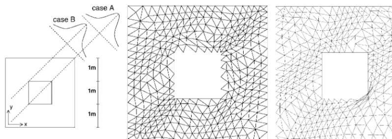
Figure 1. Square with a hole—geometry and temperature elds (left),r-adapted mesh for case A (centre) and r-adapted mesh for case B (right).

Firstly, adaptive strategies can be used to attain a prescribed accuracy. This goal is best

met with an h-, p- or hp-adaptive scheme in combination with a sound error estimator. These

schemes enable the addition and deletion of degrees of freedom, and the mesh connectivity is allowed to change. As a consequence, these schemes oer topological exibility, but the expenses in terms of computer time associated to these adaptive techniques are relatively high [2].

Secondly, adaptive strategies may be used in order to limit the computer costs. For

large-scale three-dimensional analyses mesh optimization can reduce the computer time and mem-ory requirements of an analysis by several orders of magnitude. For instance, a signicant

speed-up of the computational process can be obtained by an r-adaptive scheme such as

the Arbitrary Lagrangian–Eulerian (ALE) method [6; 7]. The constant number of degrees of

freedom and the constant element connectivity make these methods inexpensive. Since the

computational costs involved with ALE remeshing can be made as low as O(N), with N

the number of nite elements, the overhead of r-adaptive remeshing included in a nite

el-ement implel-ementation can be made negligible [8; 9]. However, the xed number of degrees

of freedom and mesh connectivity limit the applicability of r-adaptive remeshing. This is

illustrated in Figure 1, where r-adaptivity is used to optimize a nite element discretization

of a thermal problem. (Details of this problem can be found in Section 5.) The solution for the temperature follows a bell-shaped prole along the main diagonal from upper left to lower right. If the bell-shape is centred at the main diagonal from lower left to upper right

(cf. case A in Figure 1, left), then r-adaptivity is an eective tool to improve the

discretiza-tion (Figure 1, centre). On the other hand, if the centre of the bell-shape is shifted upwards (cf. case B in Figure 1, left), the non-convex corners of the hole lead to element

entan-glement when r-adaptivity is used (Figure 1, right). Thus, the applicability of r-adaptivity

is limited.

The properties and the application elds of both types of adaptive schemes (sophisticated, expensive schemes versus inexpensive schemes of limited applicability) are thus complemen-tary. This has led to the idea that the advantageous properties of both schemes could be combined. Each scheme should be used where and when it is suited most. Combinations of

dimensions [10–12]. The focus of this paper will be on combined rh-adaptive schemes for nite element analysis.

The approach followed is to decompose the domain into two subdomains. The rst sub-domain consists of all regions in the sub-domain where the element sizes are close (to a certain

extent) to the desired element sizes. In these regions, node relocation (r-adaptivity) based on

the ALE technique is carried out. The second subdomain contains the remainder of the

do-main, where element sizes dier signicantly from the desired element sizes. Here, h-adaptive

mesh renement or mesh de-renement is applied. The subdivision of the domain is based

on the concept of a desired element size, which is a common ingredient in most error

assess-ment procedures. Thus, the approach can be generalized to various elds of application. A numerical parameter can be provided by the user which sets the bounds of the criterion with

which an element is assigned to the r-adaptive subdomain or to the h-adaptive subdomain.

When this parameter favours larger r-adaptive subdomains, consequently more emphasis is

put on computational speed-up and less on numerical accuracy. Conversely, other values for this parameter lead to a larger relative importance of numerical accuracy as compared to computational speed-up. Thus, the user can control the relative importance of attaining a pre-scribed accuracy and speeding-up the computational process, and a more exible formulation of adaptive strategies is obtained.

In the present study, only linear examples are treated where the exact error is known. If the approach is to be extended to other application elds, then error estimators and error indicators must be included [2]. However, the complete proposed algorithm is based on the formulation of a desired element size, by which extension to other error assessment tools is straightforward. In case of a non-linear analysis also an algorithm for the transfer of the

state variables must be provided [8; 13]. The focus of this paper is on the subdivision of

the domain and the construction of a new discretization. Application of error estimators and error indicators and the inclusion of a transfer algorithm will be dealt with in a forthcoming contribution.

The present paper is organised as follows. First, error assessment is discussed, as well as how an optimal element size can be derived. Next, the subdivision of the domain into

an h-adaptive subdomain and an r-adaptive subdomain is treated. This subdivision is based

on error assessment. Then, the generation of a new discretization for the two subdomains is treated. Two-dimensional examples are presented to illustrate the approach. Open questions and future developments are addressed next.

2. ERROR ASSESSMENT AND OPTIMAL ELEMENT SIZES

The basis of any adaptive strategy is error assessment. It must be known in which regions of the domain the discretization is ne enough, in which regions renement is needed, and in which regions de-renement can be accepted. In general, three methods of assessing the error exist, where we use the classication of Huerta and coworkers [2]:

• For a small subclass of (academic) problems, the exact solution is known. Then, it is

possible to compute the exact error as the dierence of the exact solution and the

• The so-callederror estimatorsapproximate the exact error. Since they providequantitative information about the exact error, error estimators can be used to reach a prescribed

accuracy. Error estimators must have a solid mathematical basis [2; 14]. The computation

of error estimators is relatively expensive.

• Finally, error indicators only give relative information about the exact error. An error

indicator is based on heuristic considerations and denotes where the error is large and

where it is small, but nothow large or small. A sound mathematical basis is lacking, and

no quantitative measure of the exact error is provided. However, an error indicator is cheap in terms of computational costs. Error indicators can be based on variations of the solution, strain projection norms, element distortion and jump or average of state variables, e.g., each of which are readily available in a nite element analysis. Contrary to error estimators, error indicators do not necessarily have an upper bound.

Once an error tolerance is set, an optimality criterion can be used to translate the (exact or

estimated) error distribution into a eld of desired element size. If an error indicator is used, the user has to specify a coupling between error indicator and desired element size. In this

paper, only exact errors are used, therefore a mathematically based optimality criterion will

be used.

Several methods exist to relate the exact error or the estimated error to an element size that is expected to meet the accuracy requirements [15–19]. It has been shown that the optimality

criterion proposed in References [15; 16] leads to meshes with the lowest number of elements.

The desired size hdes _{for element i is related to the current size h}cur _{of element i according}

to [15; 16; 19]

hdes

i =hcuri √_NÁ_desku_kk_ek i

!_1=(p+d=2)

(1)

where h is a characteristic element size such as the diameter,Á is the prescribed relative error

(prescribed accuracy), p is the maximum degree of the complete interpolation polynomials,

d is the number of spatial dimensions, kuk andkeki are the energy norm of the solution eld

u for the whole domain and the local errore for element i, respectively, dened via

kak2

i =

Z

i

∇aC∇ad and kak2₌NPcur

i=1kak 2

i (2)

with C the discretised Jacobian of the problem (the tangent stiness matrix) and Ncur _the

current number of elements. In Equation (2) it is assumed that C is positive denite. It can

be seen from Equation (1) that a larger error tolerance Áleads to larger values for the desired

element size. On the other hand, a larger local error kek2

i leads to a smaller desired element

size. In Equation (1), Ndes _{is the desired number of elements, given by [15]}

Ndes₌ NPcur

i=1

keki Ákuk

d=(p+d=2)!1+d=2p

(3)

Note that the desired number of elements increases with a decreasing error tolerance and with

increasing local errors, while it decreases for increasing values of the polynomial degree p. A

closer investigation of Equations (1) and (3) reveals that the desired element size decreases

Remark 1. Equation (1) relies on the assumption that the order of convergence of the

nite element approximation coincides with the polynomial degree p. It is well known that

this does not hold near a singularity [20], where convergence is controlled by the strength of the singularity. However, as pointed out in Reference [21], the inuence of the singularity on the solution decreases during the adaptive renement. For this reason, Equation (1) is used all over the domain to keep the remeshing process as simple as possible.

3. SUBDIVISION OF THE DOMAIN

When the desired element sizes have been computed, basically three types of regions in the computational domain can be distinguished:

• Regions where the current element size does not dier too much from the desired element

size.

• Regions where the current element size is signicantly smaller than the desired element

size.

• Regions where the current element size is signicantly larger than the desired element

size.

We will dene the ratio of current element size over desired element size as the Renement

Ratio:

RR= current element size

desired element size (4)

where current element size and desired element size are taken from Equation (1). The

re-nement ratio denotes whether an element has a size which is close to optimal (RR≈1), too

small (RR¡1) or too large (RR¿1). In the remainder of this paper the following idea is

applied: if the current element size is more or less optimal (RR≈1), then r-adaptivity will

be applied. If the current element size diers signicantly from the desired element size, then locally a new discretization will be constructed to meet the desired element sizes, which is

basically an h-adaptive approach. We adopt

if 0¡RR¡1= allow h-de-renement (5)

if 1=6RR6 relocate the nodes (6)

if ¡RR¡∞ apply h-renement (7)

with ¿1 a scalar parameter that can be provided by the user. Based on the distribution of

the renement ratio, the domain can be subdivided into h-adaptive regions (the h-adaptive

subdomain) and r-adaptive regions (the r-adaptive subdomain). By assigning specic values

to , the user can put a relative importance to either subdomain. For instance, taking relatively

large values for will lead to a relatively larger-adaptive subdomain. As such, the properties

of r-adaptivity (signicant computational speed-up, limited capabilities to decrease the error)

Figure 2. Smoothening of theh-adaptive (gray) and r-adaptive (white) subdomains: initial conguration (left), conguration after smoothening of the h-adaptive subdomain (centre) and conguration after

smoothening of the r-adaptive subdomain (right).

will result in larger h-adaptive subdomains, so that computational speed-up is less pronounced

but higher accuracies can be attained.

Remark 2. Note that the subdivision of the domain is based on the computed desired

element size. As such, it is independent of the error measure that is used.

The subdomains that result from Equations (5)–(7) can yield a scattered pattern of small

r-adaptive zones and small h-adaptive zones. Obviously, it is not desirable to assign a single

element with RR¿ to the h-adaptive subdomain if this element is surrounded by elements

where 1=6RR6. Therefore, both subdomains are smoothened. For the triangular elements

adopted here, this means that each element is assigned to a certain zone when at least two neighbouring elements (i.e. sharing one edge) belong to this zone. To facilitate the adjustment

of the number of elements, the h-adaptive subdomain is given preferential treatment in the

smoothening procedure. First,r-adaptive elements that have at least twoh-adaptive neighbours

are added to the h-adaptive subdomain. When this is nished, the process is reversed: each

h-adaptive element with at least two r-adaptive neighbours becomes an r-adaptive element.

In this manner, more regular subdomains are obtained, see Figure 2 for an illustration of this approach.

4. REMESHING

After the domain has been split, a new discretization must be supplied for each subdomain. Since both subdomains are disjoint, the best available remeshing tools can be applied in each case. In the current study, the interface between the two subdomains remains xed, i.e. nodes

from the intersection between the r-adaptive subdomain and the h-adaptive subdomain are

not allowed to move (no r-adaptivity), neither is it allowed that new nodes are added on the

interface (no h-adaptivity). This treatment of the interface is a rst attempt, and other options

4.1. h-adaptive subdomain

For theh-adaptive subdomain we directly apply the desired element sizes that emerge from the

Li–Bettess optimality criterion [16] (cf. Equation (1)). This distribution of desired element

sizes is used as input for the mesh generation module, by which the h-adaptive process

is nished. Consequently, the quality of the mesh generator is decisive for a successfull

application of h-adaptivity. Currently, good mesh generators are widely available for various

two-dimensional element types. Three-dimensional mesh generators that are capable of meeting prescribed desired element sizes throughout the domain are becoming also available.

4.2. r-adaptive subdomain

In the r-adaptive subdomain a dierent strategy is followed. Since no elements are added

to this subdomain, relative information is needed, that is, in which parts of the subdomain nodes should be concentrated, and from which parts of the subdomain nodes can be taken away [2]. The strategy employed here is the equidistribution of a relocation indicator. The

relocation indicator, denoted K, takes large values where small elements are desired and vice

versa. Equidistribution of this relocation indicator is stated as [22; 23]

Kii=Kjj or

Z

i

Kd =Z j

Kd ∀i; j (8)

with i the volume of element i. Equation (8) can be rewritten in a dierential format as

[23]

@ @

K(x)@x_@

= 0 (9)

which is used to solve for the nodal positions x. Equation (9) can be repeated for each spatial

co-ordinate, so that generalization towards two and three-dimensional problems is

straightfor-ward. The co-ordinates in Equation (9) denote a reference system with respect to which

the node relocation is carried out. This co-ordinate system must be chosen independent of the spatial co-ordinates, and remains xed throughout the analysis [22–25]. Normally, the initial

nodal positions are taken for . Then, the best choice for K would be the inverse of the

desired element size:

K=_{desired element size}1 (10)

It can be seen directly from Equation (8) that equidistribution then leads to an optimal mesh, i.e. where each element takes its desired size, provided that the total number of elements is large enough.

It is also possible to take the current nodal positionsxcur _{instead of in Equation (9) if the}

change of the reference system is accounted for. This is highly advantageous, since then the

initial co-ordinates need not be stored. Furthermore, in a combined rh-adaptive approach it can

be a cumbersome task to assign a referential co-ordinate (which is needed for r-adaptivity)

to a node that has been added (by means of h-adaptivity) in an intermediate stage of

term in Equation (9) gives

@ @xcur

K(x)_@x@x_cur@x_@cur

@xcur

@ = 0 (11)

The factor @xcur_{=@ is proportional to the current element size and it is non-zero. If we}

substitute Equation (10) into Equation (11) and dene a new relocation indicator ˜K as

˜

K= current element size_{desired element size}=RR (12)

then a new equidistribution dierential equation is found with a format similar to that of Equation (9):

@ @xcur

RR(x)_@x@x_cur

= 0 (13)

Note that Equation (13) only contains quantities of the current conguration, and is based on the computation of a desired element size. Thus, generality is preserved.

Remark 3. Equation (13) represents a non-linear system of equations, which has to be

solved in ther-adaptive subdomain. Explicit algorithms have been devised to solve this system

with the order of the computational costs O(N), where N is the number of elements involved.

Thus, the remeshing in the r-adaptive subdomain is highly ecient [9; 22].

Remark 4. Equation (9) as well as Equation (13) must be solved together with a set of

boundary conditions. These boundary conditions are normally taken as prescribing for all boundary nodes a zero displacement normal to the boundary [24].

Remark 5. Since dierent stages in the analysis may lead to dierent subdivisions of the

domain, a varying r-adaptive subdomain is taken as the basis of solving Equation (13). For

a straightforward implementation Equation (13) can also be solved on the complete domain,

provided that all nodes of the h-adaptive subdomain are considered to be boundary nodes and

are, thus, xed (in all spatial directions).

Remark 6. In Equation (13), no assumptions have been made on the element type that is

used. Indeed, the remeshing strategy of the r-adaptive subdomain is valid for any element

type (in contrast, mesh generators for h-adaptive remeshing do depend on the applied element

type).

5. EXAMPLES

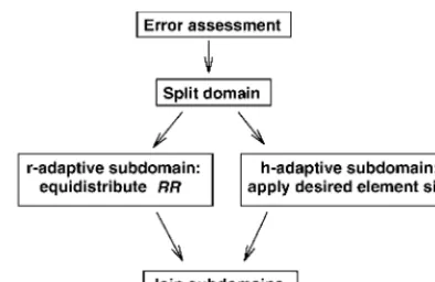
The algorithm is summarised in Figure 3. This algorithm has been implemented in the

object-oriented nite element code CASTEM 2000 [26]. Linear triangular elements have been taken.

Linear thermal problems with known analytical solution have been used to test the algorithm.

In Section 5.1, we have taken the subdivision parameter constant, while the eect of a

Figure 3. Algorithm.

5.1. Fixed subdivision parameter

The rst example deals with a rectangular strip with height = 4 m and width = 1 m. The

con-ductivity of the material c= 1 W=mK. If the origin of the axes is located at the centre of the

strip with the y-axis parallel to the longer side of the specimen, the exact temperature eld

uexact is expressed as uexact= 5 exp(−2y2) K. The numerical solution unum follows from the

partial dierential equation

c∇2_u

num= −q (14)

with −q, a source term which is taken as the second derivative of uexact times c. Essential

boundary conditions u are imposed as u=uexact on the boundary of the domain. A relative

error tolerance Á= 0:05 has been prescribed (cf. Equation (1)). As an illustration of the rh

-adaptive algorithm an analysis has been performed with = 2:5.

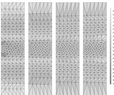
The distribution of the energy norm of the error (cf. Equation (2) with e=uexact−unum)

is depicted in Figure 4a. From this error distribution the renement ratio has been computed (Figure 4b), after which the domain is split (Figure 4c). A new discretization is constructed

based on h-adaptivity in the central part and based on r-adaptivity in the outermost parts (see

Figure 4d). The two subdomains are joined and taken as input again for the same analysis. This procedure is repeated four times. The consecutive error distributions are plotted in Figure

5. After the rst remeshing step all elements’ renement ratios fall within the interval [1=; ],

so that only node relocation is performed in the later stages. Thus, the topology of the initial mesh is preserved in the outermost parts of the domain throughout the analysis.

The development of the energy norm of the error kek, given by (cf. Equation (2))

kek2₌NPcur

i=1kek 2

i (15)

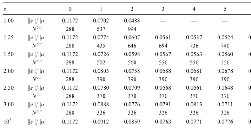
is shown in Table I. The table gives the development of the error and the number of elements

for dierent values of . In this table, the integer column headers denote the analysis index, i.e.

a ‘0’ denotes the initial computation, a ‘1’ denotes the computation after one step remeshing,

etc. A fullh-adaptive analysis (= 1) and a fullr-adaptive analysis (= 102_{) have been added}

Figure 4. Example of a strip—energy norm of the error (a), renement ratio (b), splitting the domain (c) and remeshing (d).

remeshing step. The relative errors and numbers of elements are summarized in Figure 6,

where the mesh convergence behaviour for dierent values of is depicted.

Examining Table I and Figure 6, it can be concluded that lower values of(relatively much

h-adaptivity, relatively little r-adaptivity) lead to higher accuracies. The lower the value of ,

the lower the relative error becomes. For these lower values of more elements are added

during the analysis. For higher values of the eect ofr-adaptivity is more pronounced, which

can be seen from the longer vertical line segments in Figure 6. Although for higher values of

, the number of elements is invariant during the later stage of computation, still a signicant

increase in accuracy can be obtained. Indeed, the mesh convergence of the rh-approach is

higher than that of the pure h-adaptive technique, and for the higher values of the mesh

convergence improves.

Discrepancies from the general tendency (higher accuracy for lower values of , higher

eciency for higher values of ) are caused by a more scattered subdivision of the domain.

For instance, the overall performance of = 2:0 is worse than that of = 2:5. In the rst

case the h-adaptive subdomain and the r-adaptive subdomain consist of more parts than for

Figure 5. Example of a strip—error distribution after one, two, three and four steps remeshing (a–d, respectively).

form, which poses more constraints on the h-adaptive remeshing as well as on the r-adaptive

remeshing. The same reasoning holds for the analysis with = 3:0, where a temporary decrease

of accuracy is followed by an increase of accuracy (see Table I). The obtained accuracy can be improved by articially decreasing the prescribed relative error. Thus, while we still aim

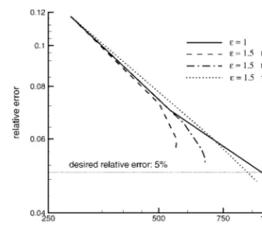
at a relative error of 5 per cent, we impose a lower value for Á. Figure 7 shows the mesh

convergence behaviour for analyses with = 1:5 when Á is varied. We observe a gradual

decrease of the nal error, while the mesh convergence behaviour is still better than that

of the full h-adaptive analysis. For Á= 0:04 the relative error is below the desired value of

5 per cent.

Figure 8 shows the mesh developments for two dierent prescribed relative errors, Á= 0:05

and 0.025, respectively, and = 2. In the rst remeshing step with Á= 0:05 four r-adaptive

zones can be recognized, separated by three h-renement zones in the centre and two h

-de-renement zones at the extremes of the domain. On the other hand, in the Á= 0:025 analysis

Table I. Example of a strip—relative error kek=kuk and number of elementsNcur _{for dierent values of .}

0 1 2 3 4 5 6

1.00 kek=kuk 0.1172 0.0702 0.0488 — — — —

Ncur _{288 537 994}

1.25 kek=kuk 0.1172 0.0774 0.0607 0.0561 0.0537 0.0524 0.0514

Ncur _{288 435 646 694 736 740 738}

1.50 kek=kuk 0.1172 0.0726 0.0598 0.0567 0.0563 0.0560 0.0558

Ncur _{288 502 560 556 556 556 556}

2.00 kek=kuk 0.1172 0.0805 0.0738 0.0688 0.0681 0.0678 0.0676

Ncur _{288 390 390 390 390 390 390}

2.50 kek=kuk 0.1172 0.0780 0.0709 0.0668 0.0661 0.0648 0.0638

Ncur _{288 370 370 370 370 370 370}

3.00 kek=kuk 0.1172 0.0888 0.0776 0.0791 0.0813 0.0711 0.0699

Ncur _{288 326 326 326 326 326 326}

102 _{kek=kuk 0.1172 0.0912 0.0859 0.0763 0.0771 0.0776 0.0778} Ncur _{288 288 288 288 288 288 288}

Figure 6. Example of a strip—mesh convergence for dierent values of.

domain. For both analyses most of the h-adaptation takes place in the rst remeshing step. In

subsequent steps, the majority of the domain belongs to the r-adaptive subdomain.

In a second example, we study the evolution of the error in the two subdomains. The geometry is shown in Figure 9. We follow the same approach as in the previous example,

now with uexact= 5 exp(−5y2) K and c= 1 W=mK. The desired relative error is Á= 0:05, so

thatÁkuk= 0:497. Two values for have been compared, namely= 1:5 and = 2:0. In Figure

10, the subdivision of the domain into an h-adaptive subdomain and anr-adaptive subdomain

Figure 7. Example of a strip—mesh convergence for dierent values of Á.

We compute the norm of the error in theh- and the r-adaptive zones separately in order to

illustrate how the error evolves in each subdomain. This cannot be done in a straightforward

manner, since the h-adaptive zones and the r-adaptive zones themselves evolve during the

adaptive process. Thus, the error in each subdomain changes from one mesh to another due to (i) remeshing and (ii) a changing subdivision of the domain. Therefore, the subdomains must be ‘xed’ for a correct investigation of the error development in each subdomain. We

have projected the error distribution onto the subdomains of the previous mesh. For instance,

the error in the r-adaptive subdomain of the initial mesh (Figure 10, top row) is compared to

exactly the same area of the domain, but now taken from the mesh after remeshing (Figure

10, middle row). In this manner, the error development in both subdomains can be measured in an objective sense. Table II shows the energy norm of the error in the whole domain, the

r- and the h-adaptive subdomain, as well as the number of elements of each of these domains.

Note that kek2_=kek2

r+kek2h (cf. Equation (2)). From the number of elements as well as from

Figure 10 it can be seen that the r-adaptive subdomain grows with respect to the h-adaptive

subdomain for ongoing remeshing steps. For larger the r-adaptive subdomain is larger. The

error norms show that large decreases in error can be obtained in the h-adaptive subdomain,

whereas the accuracy gain in the r-adaptive subdomain is smaller.

Thirdly, the example of Section 1 is analysed again, but now with the combinedrh-adaptive

approach. The geometry can be found in Figure 1, while we take the loading conditions of

case B. As such, the exact temperature elduexact= 3 exp(−1:5s2) wherebys=1₂√2(x−y−1).

Furthermore, the conductivity c= 1 W=mK. Again, the desired relative error Á= 0:05. Figure

11 shows the relative error as a function of the number of elements for various values of .

Basically, the same trends as with the other examples are found. Larger values for lead to

higher rates of mesh convergence, while lower values for lead to higher nal accuracies.

In Figure 12, the nal meshes for the various values of have been plotted. Note that the

purely r-adaptive approach (= 100) leads to element entanglement for this example (see

also Figure 1, right). Furthermore, the analysis with = 2 leads to some very badly shaped

elements around the lower-right corner of the hole. This demonstrates the need for a certain

Figure 8. Example of a strip—mesh development for= 2, prescribed relative errorÁ= 0:05 (top row) andÁ= 0:025 (bottom row).

5.2. Varying subdivision parameter

In the previous section, the subdivision parameter has been xed. In this section, the eect

of a varying is studied. Two strategies are proposed, which follow dierent reasonings. The

Figure 9. L-shape example—geometry.

For the rst approach we have taken an expression for that decreases with a decreasing

error as

=_Ák_ke_uk_k (16)

In the limit state, i.e. askek approachesÁkuk,goes to one. Consequently, the interval [1=; ]

on basis of which elements are assigned to the r-adaptive subdomain becomes smaller and

smaller. In other words, a signicant part of the domain will remain h-adaptive (contrary to

the case of a xed value for , see Section 5.1). Thus, the number of elements can easily be

adjusted in all remeshing steps. The example of the strip is analysed again but now with

ac-cording to Equation (16). The desired relative errorÁ= 0:05. The mesh convergence behaviour

is depicted in Figure 13. As a reference also the case of a xed = 1:0 (full h-adaptive) is

plotted in this gure. It can be seen that the mesh convergence behaviour is not an

improve-ment of the results obtained with a xed (cf. Figure 6). Although elements are added in

all remeshing steps, the numerical error arrests at a certain stage and does not decrease any-more. The reason for this behaviour is the relatively complex form of the interface between

the h-adaptive subdomain and the r-adaptive subdomain. Whereas for a ÿxed this interface

becomes more and more simple and eventually disappears (see Figure 10, for instance),

a decreasing maintains a signicant h-adaptive subdomain even in later remeshing steps. As

a consequence, the interface between the r-adaptive subdomain and theh-adaptive subdomain

does not disappear but remains of relatively complex form. This poses topological constraints

on the h-adaptive remeshing as well as on the r-adaptive remeshing, by which the decrease

in error is severely reduced. To mitigate this deciency, more exible formulations of the interface should be considered. However, this falls beyond the scope of the present study.

A totally dierent approach is to let increaseduring the analysis. This is motivated by the

fact that a small (much h-adaptivity) in the rst remeshing steps is more suitable to meet

the desired number of elements more precisely in an early stage of the analysis, whereas a

larger (much r-adaptivity) in later remeshing steps facilitates the ne-tuning of the nodal

co-ordinates. Thus, the interface between the two subdomains has a less complicated form

Figure 10. L-shape example—subdivision into h-adaptive subdomain (gray) and r-adaptive subdomain (white) for= 1:5 (left column) and= 2:0 (right column); ini-tial mesh (mesh 0—top row), mesh after one remeshing step (mesh 1—middle row)

and mesh after two remeshing steps (mesh 2—bottom row).

the remeshing process. We have adopted the following denition of :

=Á_ÿk_ku_ek_k + 1 (17)

where ÿis a numerical parameter. Note that ≈1 for relatively large values of kek, whereas

→1=ÿ+ 1 if kek approaches Ákuk. Thus, goes to 2 if ÿ= 1, goes to 1.5 if ÿ= 2, etc.

The mesh convergence behaviour of the strip example with Á= 0:05 for an increasing is

Table II. L-shape example—error development and number of elements.

Step 1 Step 2 Step 3

Mesh 0→Mesh 1 Mesh 1→Mesh 2 Mesh 2 →Mesh 3

= 1:5 kek 1.02592 0.92105 0.92105 0.59855 0.59855 0.57943

Ncur _{852 821 821 1245 1245 1247}

kekr 0.25229 0.24051 0.43249 0.40300 0.59222 0.57271

Ncur

r 230 230 538 538 1221 1221

kekh 0.99442 0.88909 0.81319 0.44255 0.08683 0.08799

Ncur

h 622 591 283 707 24 26

=2.0 kek 1.02592 0.85628 0.85628 0.75951 0.75921 0.69872

Ncur _{852 740 740 844 844 844}

kekr 0.59277 0.51634 0.64836 0.64987 0.75921 0.69872

Ncur

r 487 487 665 665 844 844

kekh 0.83734 0.68309 0.55932 0.39310 0 0

Ncur

h 365 253 75 179 0 0

Figure 11. Square with a hole—mesh convergence for xed values of.

for increasing is better than that of a full h-adaptive analysis. For the case →1:25 (ÿ =

4) the desired relative error is met. Compared to the xed case, more elements are added

in an early stage of the analysis, so that the nal error is lower.

Also, the example of the square with a hole is analysed with the increasing according

to Equation (17). Figure 15 shows the mesh convergence behaviour for various values of ÿ,

whileÁ= 0:05. For the case→1:25 the error tolerance is met. Compared to the corresponding

analyses with xed values of (see Figure 11), the mesh convergence rate is somewhat

Figure 12. Square with a hole—nal meshes for = 100 (top left), = 2 (top right), = 1:5 (bottom left) and = 1:25 (bottom right).

6. DISCUSSION

The paper aims to combine the advantageous properties of two adaptive strategies, namely,

node relocation (r-adaptivity) and adjusting element sizes and mesh topology (h-adaptivity).

Basically, r-adaptive strategies are recognized to be computationally inexpensive but with

lim-ited applicability, whereas h-adaptive strategies are suitable for meeting a prescribed accuracy

at the cost of a higher computational eort.

In the current study, the domain under consideration is split into two subdomains. In the regions where the element sizes do not dier too much from the desired element sizes node

relocation is applied. In the remainder of the domain, an h-adaptive approach is chosen. The

subdivision of the domain as well as the construction of a new discretization in both subdo-mains is based on the computation of a desired element size, so that generality is preserved.

Through this domain subdivision, each remeshing technique (r-adaptivity, h-adaptivity) can

be used in the subdomain where it is suited most.

Figure 13. Example of a strip—mesh convergence for a decreasing according to Equation (16).

Figure 14. Example of a strip—mesh convergence for an increasing according

to Equation (17).

Figure 15. Square with a hole—mesh convergence for an increasing according

to Equation (17).

is desired. As such, the present approach can be regarded as an enhancement of the h

-adaptive nite element method in which parts of the domain are remeshed with the cheaper

r-adaptive technique. Conversely, the proposed combined rh-adaptive strategy may be seen

as an extension of r-adaptive approaches, namely where h-adaptivity is used if r-adaptivity is

deemed unsuitable.

A numerical parameter has been introduced that can be set by the user in order to at-tach more importance to accuracy or to computational speed-up. Alternatively, this parameter

can be computed as a function of the error level. If more weight is put on h-adaptivity,

Conversely, if r-adaptivity is emphasized, then the mesh convergence behaviour is better

while attaining a prescribed error level may become impossible. Compared to a purely h

-adaptive technique, the computational costs are lower in the combined rh-adaptive approach.

With a suitable choice for the above-mentioned numerical parameter the same accuracy can be obtained with a smaller number of nite elements. On the other hand, the

pro-posed combined rh-adaptive strategy oers better accuracies than a purely r-adaptive

approach.

Features that will be addressed in the future include the following:

• The treatment of the intersection between the r- and the h-adaptive subdomain has not

been investigated in depth. In the present study, only a xed interface is considered, which

can have an interfering eect on the adaptivity process in ther-adaptive subdomain as well

as the h-adaptive subdomain. Future investigations should include r- and=or h-adaptivity

at the intersection.

• Using the numerical parameter as a criterion to split the domain has been a rst attempt.

More sophisticated algorithms may be used and compared. Furthermore, the case of a

decreasing value for the subdivision parameter should be studied in combination with

a less rigid treatment of the interface between the two subdomains. It is expected that

through this combination the mesh convergence behaviour of rh-adaptive schemes can be

improved.

• In the present study, only exact errors have been used. The performance of the proposed

rh-adaptive strategy should also be assessed with error estimators and error indicators.

• The extension towards non-linear problems requires an algorithm to transfer the state

variables. As with the adaptation of the mesh dierent stress transfer algorithms can be used that suit the two subdomains best.

ACKNOWLEDGEMENTS

We wish to thank Pedro Dez and Antonio Huerta for the various technical discussions. Furthermore, we gratefully acknowledge the Commissariat a l’ Energie Atomique, France, for the availability of the nite element code CASTEM 2000.

REFERENCES

1. Zienkiewicz OC, Zhu JZ. Adaptivity and mesh generation. International Journal for Numerical Methods in Engineering1991;32:783–810.

2. Huerta A, Rodrguez-Ferran A, Dez P, Sarrate J. Adaptive nite element strategies based on error assessment.

International Journal for Numerical Methods in Engineering1999;46:1803–1818.

3. Ladeveze P, Rougeot Ph, Blanchard P, Moreau JP. Local error estimators for nite element linear analysis.

Computer Methods in Applied Mechanics and Engineering1999;176:231–246.

4. Babuska I, Strouboulis T, Gangaraj SK, Upadhyay CS. Pollution error in theh-version of the nite-element method and the local quality of the recovered derivatives. Computer Methods in Applied Mechanics and Engineering1997;140:1–37.

5. Hager P, Wiberg N-E. Adaptive eigenfrequency analysis by superconvergent patch recovery.Computer Methods in Applied Mechanics and Engineering1999;176:441–462.

6. Hughes TJR, Liu WK, Zimmermann TK. Lagrangian–Eulerian nite element formulation for incompressible viscous ows.Computer Methods in Applied Mechanics and Engineering1981;29:329–349.

7. Donea, J. Arbitrary Lagrangian–Eulerian nite element methods. In Computational Methods for Transient AnalysisChapter 10, Belytschko T, Hughes TJR (eds). Elsevier: Amsterdam, 1983; 474–516.

9. Askes H, Sluys LJ. Remeshing strategies for adaptive ALE analysis of strain localisation.European Journal of Mechanics A=Solids 2000;19:447–467.

10. Cao T. Adaptive H- and H-R methods for Symm’s integral equation.Computer Methods in Applied Mechanics and Engineering1998;162:1–17.

11. Ammons BA, Vable M. Anhr-method of mesh renement for boundary element method.International Journal for Numerical Methods in Engineering1998;43:979–996.

12. Kita E, Higuchi K, Kamiya N. r- and hr-adaptive boundary element method for two-dimensional potential problem.Computers and Structures 2000;74:11–19.

13. Ortiz M, Quigley JJ. Adaptive mesh renement in strain localization problems. Computer Methods in Applied Mechanics and Engineering1991;90:781–804.

14. Dez P, Egozcue JJ, Huerta A. A posteriori error estimation for standard nite element analysis. Computer Methods in Applied Mechanics and Engineering1998;163:141–157.

15. Li LY, Bettess P. Notes on mesh optimal criteria in adaptive nite element computations. Communications in Numerical Methods in Engineering1995;11:911–915.

16. Li LY, Bettess P, Bull JW, Bond T, Applegarth I. Theoretical formulations for adaptive nite element computations.Communications in Numerical Methods in Engineering 1995;11:857–868.

17. Zienkiewicz OC, Zhu JZ. A simple error estimator and adaptive procedure for practical engineering analysis.

International Journal for Numerical Methods in Engineering1987;24:337–357.

18. O˜nate E, Bugeda G. A study of mesh optimality criteria in adaptive nite element analysis. Engineering Computations1993;10:307–321.

19. Dez P, Huerta A. A unied approach to remeshing strategies for nite elementh-adaptivity.Computer Methods in Applied Mechanics and Engineering1999;176:215–229.

20. Zhu JZ, Zienkiewicz OC. Adaptive techniques in the nite element method. Communications in Applied Numerical Methods1988;4:197–204.

21. Zienkiewicz OC, Zhu JZ. Error estimates and adaptive renement for plate bending problems. International Journal for Numerical Methods in Engineering1989;28:2839–2853.

22. Bode L. Strategies numeriques pour la prevision de la ruine des structures du genie civil. Dissertation E.N.S. de Cachan=CNRS=Universite Paris 6, 1994.

23. Pijaudier-Cabot G, Bode L, Huerta A. Arbitrary Lagrangian–Eulerian nite element analysis of strain localization in transient problems.International Journal for Numerical Methods in Engineering1995;38:4171–4191. 24. Huerta A, Casadei F. New ALE applications in non-linear fast-transient solid dynamics. Engineering

Computations1994;11:317–345.

25. Huerta A, Liu WK. Viscous ow with large free surface motion. Computer Methods in Applied Mechanics and Engineering1988;69:277–324.