Resource Allocation in Streaming Environments
Thesis by
0
•
(Lu Tian)
In Partial Fulfillment of the Requirements for the Degree of
Master of Science
California Institute of Technology Pasadena, California
2006
© 2006
Acknowledgements
First, I would like to thank my advisor, Professor K. Mani Chandy, for giving me tremendous support and guidance throughout the years of my graduate study. I feel extremely fortunate and honored to be his student and have the opportunity to work with him. He is not only an advisor and a friend, but also my role model. I especially want to thank him for the great effort he puts into helping his students find and achieve their personal goals in life.
I would also like to thank the members of my group—Mr. Agostino Capponi, Mr. Andrey Khorlin, and Dr. Daniel M. Zimmerman—for their help and collaboration, and their effort in creating an excellent working environment.
I must also acknowledge my good friends Patrick Hung, Kevin Tang, and Daniel M. Zim-merman for their great support, help, and friendship throughout the years, especially their excellent advice and inspiration regarding my thesis work.
Last but not least, I want to thank my family, my mother}B•, my father0· , and my twin sister0vfor always being there for me with remarkable support and understanding.
Abstract
The proliferation of the Internet and sensor networks has fueled the development of applica-tions that process, analyze, and react to continuous data streams in a near-real-time manner. Examples of such stream applications include network traffic monitoring, intrusion detection, financial services, large-scale reconnaissance, and surveillance.
Unlike tasks in traditional scheduling problems, these stream processing applications are interacting repeating tasks, where iterations of computation are triggered by the arrival of new inputs. Furthermore, these repeated tasks are elastic in the quality of service, and the economic value of a computation depends on the time taken to execute it; for example, an arbitrage opportunity can disappear in seconds. Given limited resources, it is not possible to process all streams without delay. The more resource available to a computation, the less time it takes to process the input, and thus the more value it generates. Therefore, efficiently utilizing a network of limited distributed resources to optimize the net economic value of computations forms a new paradigm in the well-studied field of resource allocation.
Contents
Acknowledgements iii
Abstract iv
List of Figures viii
1 Introduction 1
1.1 Motivation . . . 1
1.2 Thesis Structure . . . 3
2 Resource Allocation on Heterogeneous Computing Systems 4 2.1 Scheduling Heuristics . . . 4
2.1.1 Engineering Heuristics . . . 4
2.1.1.1 Bin-Packing Heuristics . . . 5
2.1.1.2 Min-Min and Max-Min Heuristics. . . 5
2.1.1.3 Genetic Algorithm and Simulated Annealing . . . 6
2.1.2 Scheduling Periodic Tasks . . . 8
2.1.2.1 Scheduling Periodic Tasks on a Single Processor. . . 8
2.1.2.2 Scheduling Periodic Tasks on Multiprocessor Systems . . . 8
2.2 State-of-the-Art Resource Management Systems . . . 10
2.2.1 Spawn . . . 10
2.2.2 MSHN. . . 11
2.2.3 Tycoon . . . 12
2.2.4 Summary . . . 13
3 Problem Formulation 14 3.1 Computational Fabric . . . 14
3.2 Streaming Application . . . 14
3.3 Proposed Solution Space: Resource Reservation Systems . . . 15
4 Market-Based Heuristics 21
4.1 Single Market Resource Reservation System . . . 25
4.1.1 Algorithm . . . 26
4.1.2 Lower Bound Analysis . . . 26
4.2 Multiple Market Resource Reservation System. . . 28
4.3 Summary. . . 30
5 Simulations 31 5.1 A Motivating Example . . . 31
5.2 Heavy-tail Distribution . . . 33
5.3 Uniform Distribution . . . 34
5.3.1 Comparison Among the Three Heuristics . . . 34
5.3.2 The Effect of Number of Machines on Performance . . . 35
5.3.3 The Effect of Total System Resource on Performance . . . 39
5.3.4 The Effect of Utility Functions on Performance . . . 41
5.3.4.1 Choice ofa. . . 41
5.3.4.2 Choice ofb . . . 44
5.3.5 Timing Analysis for the Multiple-Market Heuristic . . . 47
6 Conclusion 49 6.1 Summary. . . 49
6.2 Applications. . . 50
6.3 Future Directions . . . 51
List of Figures
2.1 An example showing poor RM scheduling performance. . . 9
3.1 Two streaming applications . . . 15
3.2 Utility functions . . . 16
3.3 System view of the solution space . . . 17
3.4 Per-machine view of the solution space. . . 17
3.5 Example of a mapping problem and a possible solution . . . 18
4.1 Demand, supply and optimal allocations. . . 22
4.2 The interpolation method for updating the market price . . . 24
4.3 System view of the single-market method . . . 25
4.4 System view of the multiple-market method . . . 29
5.1 Utility functions forT1. . . T4 . . . 32
5.2 Performances of the three heuristics under a heavy-tail stream distribution. . . 33
5.3 Performances of the three heuristics under a uniform stream distribution, with various numbers of machines. . . 34
5.4 The effect of number of machines on heuristic performance . . . 36
5.5 The effect of streams-to-machine-ratio on performance, by number of machines . . 37
5.6 The effect of streams-to-machine-ratio on performance, by heuristic . . . 38
5.7 The effect of total system resource on performance, by capacity (42 machines). . . 39
5.8 The effect of total system resource on performance, by heuristic (42 machines) . . 40
5.9 Performance comparison with various ranges ofa, by heuristic (42 machines) . . . 42
5.10 Performance comparison with various ranges ofa, by range (42 machines) . . . 43
5.11 Performance comparison with various ranges of b, by range (42 machines, a ∈ (0.2,0.3)) . . . 44
5.12 Performance comparison with various ranges of b, by range (42 machines, a ∈ (0.01,0.99)). . . 45
Chapter 1
Introduction
1.1
Motivation
The resource allocation problem is one of the oldest and most thoroughly studied problems in computer science. It is proven to be NP-complete [11,13] and therefore computationally in-tractable. Thus, any practical scheduling algorithm presents a tradeoff between computational complexity and performance [6,15]. There have been several good comparisons [3,10,23] of the more commonly used algorithms. The most common formulation of the problem in a dis-tributed computing environment is: given a set of tasks, each associated with a priority number and a deadline, and a set of computing resources, assign tasks to resources and schedule their executions to optimize certain performance metrics. These optimizations include maximizing the number of tasks that can be processed without timing/deadline violations, minimizing the
makespan(the total completion time of the entire task set), minimizing the aggregate weighted completion time, and minimizing computing resources needed to accommodate the executions of a set of tasks to meet their deadlines.
post-processing on the data streams may be carried out for data mining, pattern discovery, and model building.
Stream processing applications differ from tasks in the traditional scheduling problem in the following aspects:
• Each is a repeating task triggered by inputs arriving at a specified rate, or arriving at random intervals with a known or unspecified probability distribution.
• Instead of having hard deadlines, tasks are elastic in quality of service (QoS), and the economic value of each computation depends on the time taken to execute it; for example, the value of delivering a stock tick stream to a user with a 10-second delay is less than that with a 1-second delay.
• There can be interdependences and communication among stream processing applica-tions.
Therefore, the conventional models and their solutions are not applicable for the new problem:
• Associating each task with a single deadline is not suitable because the computations have elastic deadlines.
• Using a priority number to indicate a task’s importance/value is not suitable because applications have elastic QoS and varying economic values depending on delay.
• The solution space of determining when and on what machine each task is to be executed is not suitable because the exact time at which each computation can start is not known
a priori.
• The objective is not to minimize the makespan, as in the conventional multiprocessor scheduling problem, but rather to optimize the net economic value of the computations.
As in most real-time systems, it is critical to find the most efficient way to optimize the ongoing resource consumption of multiple, distributed, cooperating processing units. To ac-complish this, the system must handle a variety of data streams, adapt to varying resource requirements, and scale with various input data rates. The system must also assist and coor-dinate the communication, the buffering/storage, and the input and output of the processing units.
1.2
Thesis Structure
The remainder of this thesis is structured as follows:
In Chapter2, we review the research literature on resource allocation problems in hetero-geneous computing systems.
Chapters3,4, and5are devoted to the specific problem we are addressing: resource allo-cation for streaming appliallo-cations.
In Chapter3, we start by defining the computational fabric and streaming applications, then formulate our problem as an integer optimization problem and prove that it is NP-complete. We also propose using resource reservation systems as the solution space.
In Chapter4, we present two market-based heuristics for building such resource reservation systems.
In Chapter 5, we evaluate the performances of our two market-based heuristics through computer simulations.
Chapter 2
Resource Allocation on Heterogeneous
Computing Systems
A computing system is said to be heterogeneous if differences in one or more of the follow-ing characteristics are sufficient to result in varyfollow-ing execution performance among machines: processor type, processor speed, mode of execution, memory size, number of processors (for parallel machines), inter-processor network (for parallel machines),etc.
The study of resource allocation and scheduling has transitioned from single processor sys-tems to multiprocessor syssys-tems, from offline problems to online problems, from independent tasks to interacting tasks and from one-time tasks to repeated tasks. There is a rich body of research in this problem domain. Some resource allocation methods employ conventional computer science approaches, while others apply microeconomic theory and employ market or auction mechanisms. In this chapter, we review the studies conducted in this area.
2.1
Scheduling Heuristics
As described earlier, the most common formulation of the scheduling problem in a distributed computing environment is: given a set of tasks, each associated with a priority number and a deadline, and a set of computing resources, assign tasks to resources and schedule their exe-cutions to optimize certain performance metrics. There have been several good comparisons [3,10,23] of commonly used algorithms.
2.1.1
Engineering Heuristics
2.1.1.1 Bin-Packing Heuristics
Two bin-packing heuristics—First FitandBest Fit—can be applied to solve the mapping problem. In this formulation, tasks are treated as balls and machines are treated as bins.
The First Fit heuristic is also called Opportunistic Load Balancing[4]. This is the simplest heuristic of all. It randomly chooses a task from the unmapped set of tasks and assigns it to the next available machine.
The Best Fit heuristic first calculates, for each task, the machine that can execute that task the fastest. It then assigns each task to its optimal machine.
2.1.1.2 Min-Min and Max-Min Heuristics
Min-Min Given a set of machines{M1. . . MM}, the Min-Min heuristic starts with a set of
un-mapped tasks and repeats the following steps until the set of unun-mapped tasks is empty:
1. LetETijbe the execution time of taskTi on machineMj. For each taskTi, calculate the
minimum execution time (MinETi) and its choice of machinechoicei based on the current
machine availability status:
(a) MinETi = minMj=1ETij (b) choicei = argMinETi
2. Assign the task with the smallestMinETi to its choice of machinechoicei.
3. Remove this task from the unmapped set and update the availability status of its assigned machine.
The intuition behind this method is that the Min-Min way of assigning tasks to machines mini-mizes the changes to machine availability status. Therefore, the percentage of tasks assigned to their first choice machines is likely to be higher.
Max-Min This heuristic is similar to the Min-Min heuristic. It also starts with a set of un-mapped tasks and calculates the minimum execution time and choice of machine for each task. However, instead of assigning the task with the smallestMinETi first, this heuristic
as-signs the task with the largestMinETi to its choice of machine first, then repeats the process of
updating machine availability status and calculatingMinETi for each task until the unmapped
set is empty.
avoid the situation where all shorter tasks execute first, then longer tasks execute while some machines sit idle.
We can see that MMin and Max-Min both have advantages and disadvantages. This in-spired the development of another heuristic, Duplex, to incorporate the advantages of both heuristics and avoid their pitfalls. The Duplex heuristic performs both Min-Min and Max-Min and chooses the better of the two results.
2.1.1.3 Genetic Algorithm and Simulated Annealing
Genetic Algorithm In genetic algorithms [14,19], each chromosome is a vector that encodes a particular way of mapping the set of tasks to machines. Each position in this vector represents a task, and the corresponding entry represents the machine that task is mapped to,e.g., if the
ith chromosome isc
i=[0 1 1 2 1 3 0 4 2],ci[3]=1 means that taskT3is assigned to machine
M1.
Each chromosome has a fitness value, which is the makespan that results from the mapping that chromosome encodes. The algorithm is as follows:
1. Generate the initial population,e.g., a population of 200 chromosomes following a random distribution.
2. While no stopping condition is met:
(a) Selection: Probabilistically duplicate some chromosomes and delete others. Chro-mosomes with good makespan have higher probability of being duplicated, whereas chromosomes with bad makespan have higher probability of being deleted.
(b) Crossover: Randomly select a pair of chromosomes, then randomly select a region on those two chromosomes and interchange the machine assignments on the chosen region.
(c) Mutation: Randomly select a chromosome, then randomly select a task on that chro-mosome and reassign it to a new machine.
(d) Evaluation: Evaluate the following stopping conditions:
i. The process has reached a certain number of total iterations.
ii. No change in the best chromosome has occurred for a certain number of itera-tions.
iii. All chromosomes have converged to the same mapping.
Simulated Annealing Simulated annealing [9,18] also uses chromosomes to encode the map-ping of tasks to machines. However, unlike genetic algorithms, which deal with a population of chromosomes, simulated annealing only considers one mapping at a time and uses a muta-tionprocess on that chromosome to improve its makespan. It introduces the notion of system temperature to probabilistically allow poorer solutions to be accepted at each iteration. This is an attempt to avoid being trapped at local optima and to better explore the solution space. The system temperature decreases with each iteration. The higher the temperature, the more likely it is that a worse mapping is accepted. Thus, worse mappings are likely to be accepted at system initiation, but less likely as the system evolves. The procedure is as follows:
1. Generate the initial mapping.
2. While no stopping condition is met:
(a) Mutation: Randomly select a task on the chromosome and reassign it to a new ma-chine.
(b) Acceptance decision:
i. If the new makespan is better, replace the new mapping with the old one.
ii. Otherwise, probabilistically decide whether to accept the new mapping based on makespans and system temperature.
(c) Evaluation: Evaluate the following stopping conditions:
i. The system temperature approaches zero.
ii. No change in the makespan has occurred for a certain number of iterations.
3. Output the best solution.
2.1.2
Scheduling Periodic Tasks
Aperiodic taskis a task that has an assigned period, is executed periodically, and must finish each execution before the start of the next period. That is, the deadline for the execution at each period is assigned to be the start of the next period. Periodic tasks are often scheduled preemptively using a class of algorithms known aspriority-driven algorithms [10,20,23,27]. The goal is to schedule a set of tasks such that all the deadlines are met. A task set is said to be schedulable if there exists a schedule such that all tasks can finish execution before their corresponding deadlines.
2.1.2.1 Scheduling Periodic Tasks on a Single Processor
Liu and Layland [23] proposed thedynamic priority earliest-deadline-due (EDD)algorithm. The priorities of tasks are based on their relative deadlines: the closer the deadline, the higher the priority. As its name implies, EDD schedules the task with the earliest deadline (highest priority) first. They proved that EDD is optimal among all scheduling algorithms (if a task set is schedulable, then EDD achieves a feasible schedule).
Another well-known priority-driven algorithm is the rate monotonic (RM) algorithm, also proposed by Liu and Layland. RM is a fixed-priority algorithm, where the priority for each task is defined by the fixed numberpi=1/Ti(the inverse of its period). Thus, the longer the period
of the task, the lower priority it has. The task with the highest priority (shortest period) is scheduled first.
Liu and Layland presented sufficient schedulability conditions for RM: a set of N tasks is guaranteed to meet their deadlines on a single processor under RM scheduling if system uti-lization is no greater than N(2N1 −1). This lower bound is called the minimum achievable
utilization. It is a conservative but useful test for schedulability.
Due to its low computational requirement, the RM algorithm is one of the most popular choices for scheduling real-time periodic tasks on a single processor system.
2.1.2.2 Scheduling Periodic Tasks on Multiprocessor Systems
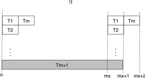
Tm+1 T1 T2 Tm o T1 T2 Tm
.
..
.
..
mx mx+1 mx+2
(a) All tasks can be scheduled onmprocessors ifTm+1has one proces-sor. Tm+1 T1 T2 Tm o T1 T2
.
..
.
..
mx mx+1 Tm mx+2 [image:17.612.201.453.56.192.2](b)Tm+1misses its deadline with RM usingmprocessors.
Figure 2.1: An example showing poor RM scheduling performance
Global Scheduling In this scheme, all tasks are stored on a centralized server and the global scheduler selects the next task to be executed on a chosen processor. The task can be pre-empted and resumed on a different processor. One of the most commonly used algorithms for the global scheduling approach is the RM algorithm. However, Dhall and Liu [22] showed that this method can result in arbitrarily low utilization if the task set containsmtasks with compute timeCi =1 and periodTi =2mxand one task with compute timeCm+1=2mx+1 and periodTm+1=2mx+1. The optimal solution is to scheduleTm+1by itself on a machine,
T1 and Tm on one machine, and T2. . . Tm−1 each on a separate machine, as shown in Figure
2.1(a). However, the RM algorithm schedules them easy tasks first because they have higher priority, and then the one hard task last (easy tasks are those with shorter periods, hard tasks are those with longer periods). As shown in Figure2.1(b), RM requires at leastm+1 processors for the task set. Total utilization of this set of tasks is
U= m X
i=1
Ci Ti
+Cm+1 Tm+1
=m 1
2mx +
2mx+1 2mx+1
= 1
Asx→ ∞, the utilization becomes arbitrarily low. Furthermore, admission control is needed to guarantee that the tasks form a schedulable set.
Partitioning Scheduling In this scheme, the problem becomes twofold:
1. Partition the set of tasks and assign the subsets to machines.
2. Schedule task executions on each machine (e.g., using the RM algorithm).
The first step, finding the optimal task assignment to machines, is equivalent to the bin-packing problem, which is proven to be NP-hard [21]. People have applied bin-packing heuristics such as First Fit and Next Fit to this problem, where the tasks are treated as balls and the machines are treated as bins. The decision of whether a bin is full is made based on the schedulability condition discussed previously. Rate Monotonic Next Fit (RMNF) andRate Monotonic First Fit (RMFF)heuristics use Next Fit and First Fit heuristics for assigning the tasks to processors, and the RM heuristic for scheduling task executions on each machine. Both of them order tasks based on the lengths of their periods. RMNF assigns new tasks to the current processor until it is full (schedulability is violated), then moves on to a new processor. RMFF tries to assign a new task to a processor that is marked as full before assigning it to the current processor. A variation of RMFF is theFirst Fit Decreasing Utility (FFDU) method. In this method, instead of being sorted according to period, tasks are sorted according toutility, which is defined as the ratio between execution time and period. This ratio is also called theload factor of a task.
As mentioned earlier, the goal of these algorithms is to minimize the number of processors needed to accommodate the executions of all the tasks. To evaluate the performances of these methods, a worst case upper bound (ratio between the number of machines needed in the worst case and the optimal solution) is used. In summary, RMNF achieves a worst case upper bound of 2.67, RMFF achieves a worst case upper bound of 2.33, and FFDU achieves a worst case upper bound of 2.0.
2.2
State-of-the-Art Resource Management Systems
2.2.1
Spawn
1. Each task bids for the next available slot on the machine where it can finish earliest.
2. Each machine chooses from the available bids to maximize its revenue, awarding exclusive usage during the next timeslot to the highest bidding task while charging the second highest price.
3. The auction is not committed until the last possible moment.
This system emphasizes economic fairness over economic efficiency. Afairresource distribu-tion is one in which each applicadistribu-tion is able to obtain a share of system resources propordistribu-tional to its share of the total system funding. Anefficientresource distribution maximizes aggregate utility (social welfare). Spawn uses a second-price auction. Thus, at any given time, there is only one auction open on each machine: bidding for the next available timeslot. This is a simple scheme, but it is not combinatorial,i.e., each winning task, whose execution may span multi-ple timeslots, is guaranteed the next available timeslot but is not guaranteed future timeslots. Therefore, a situation can occur where a task needsKtimeslots to execute, but is only able to get k < K of them before exhausting its funds. This is a major disadvantage of the second-price single-item auction compared to combinatorial auctions. Furthermore, a winning task has exclusive use of the machine during its timeslot; situations can occur where less demanding tasks do not use their entire reservations, causing low utilization.
2.2.2
MSHN
MSHN (Management System for Heterogeneous Networks) [4] is a collaborative project funded by DARPA. Its main goal is to determine the best way to support executions of many different applications in a distributed heterogeneous environment. The system uses a conventional computer science approach: it employs a centralized scheduler and uses heuristics to solve the online scheduling problem.
MSHN uses a performance metric that takes deadline, priority, and versioning into account. Performance is measured as the weighted sum of completion times, where weights are the priority numbers assigned to the tasks. Formally, performance isP
(DikPiRik), whereDikis 1
if taskiis mapped to machinekand 0 otherwise,Pi∈ {1,4,8,16}is a priority assigned by the
centralized scheduler, andRikis the time required to execute taskion machinek(entry(i, k)
in theexpected time to completionmatrix).
well enough for large systems. Finally, similar to other existing approaches, MSHN assumes that the exact time required to execute each task on each machine is known. In a streaming environment, where the arrival time of each new input is usually not known preciselya priori, this approach may not work well.
2.2.3
Tycoon
Tycoon [12] is aproportional share abstraction-based resource allocation system using an eco-nomic market-based approach, developed at HP Labs. Task owners choose computers to run their tasks and bid for resources on the chosen machines. Each bid is of the form {Bi, Ti},
whereBi is the total amount the task owner is willing to pay andTi is the time interval she
is bidding for. Machines make scheduling decisions by calculating a threshold price, Bk/Tk,
for each timeframe (e.g., 10 s) based on the collected bids. Any task with a bid above the threshold price gets a share of the machine resources proportional to the relative amount of its bid,ri =(Bi/Ti)/(Bk/Tk), and pays the machine based on its actual usage of the allocated
resources,paymenti=min(qi/rq,1)(Bi/Ti).
One drawback of this scheme is that, since payment is based on actual usage, a task’s best strategy is to bid high on all machines to guarantee a share and ensure quick execution. This results in the following two problems:
1. Tasks bid high, get large amounts of resource allocated without fully utilizing it, and pay a small amount based on actual usage; this prevents other tasks from getting reasonable shares on the machine.
2. Tasks bid high and win on all machines, and continually switch to the machine requiring the lowest payment; this results in oscillation in the system.
2.2.4
Summary
Chapter 3
Problem Formulation
There are several research projects studying various aspects of stream processing,e.g., STREAM [5], Borealis [1], SMILE [16], and GATES [8]. However, their approaches for resource management are fundamentally different from the one presented here. For example, Borealis focuses on load-balancing: minimizing end-to-end latency by minimizing load variance.
In this chapter, we first describe the components of the problem domain: the computational fabric and streaming applications. Then, we formally describe our problem as an optimization problem and propose using resource reservation systems as the solution space. Finally, we provide a formal proof of the NP-completeness of the problem.
3.1
Computational Fabric
The computational fabric for stream processing is represented by a graph, where the nodes represent processors and the edges represent communication channels. Associated with each node and each edge is a set of parameters. The parameters of a node include the amount of memory, floating-point and fixed-point speeds, etc. The parameters of an edge include bandwidth and latency.
3.2
Streaming Application
Each streaming application can be represented as having three components:
1. One or more input flows.
2. A graph of interacting processing units.
G
C1 C2
Input 1 Input 2 Input 3
G2 G1
T1 T2
T3
T4
T5
[image:23.612.213.438.66.235.2]Output 1 Output 2
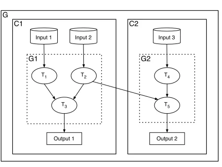
Figure 3.1: Two streaming applications
The interacting tasks are represented by a computation directed acyclic graph (DAG). The ver-tices of the graph represent tasks, and a directed edge represents flow of information from one task to another. We allow communication among applications, which means the output from one computation could be an input to another computation. Figure 3.1 shows a pair of interacting streaming applications. We model streaming applications using the following parameters:
1. Apersistence interval [Tstarti,Tendi], whereTstarti is the time instant when the application
starts receiving inputs and become active and Tendi is the time instant when it stops
receiving inputs and becomes inactive.
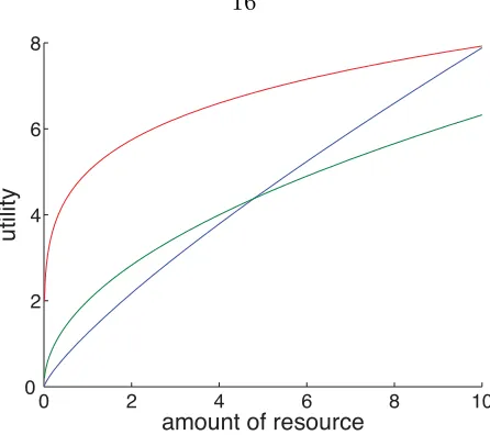
2. A utility function U (r ), which maps an amount of resource r to the value realized by processing the inputs with that guaranteed amount of resource.
For theoretical foundations about utility functions, refer to Mas-Colell, Whinston and Green [24]. In most cases,U (r )is a concave nondecreasing function with parameters that depend on the application. Figure3.2shows the utility functions of three streaming applications.
3.3
Proposed Solution Space: Resource Reservation Systems
0 2 4 6 8 10 0
2 4 6 8
amount of resource
[image:24.612.213.436.58.256.2]utility
Figure 3.2: Utility functions
If we assume that each processing unit can be split and hosted on multiple machines, then the problem becomes the following continuous convex optimization problem, which is easily solved using standard optimization techniques:
max PN
i=1Ui(ri)
subject to ri≥0,
PN
i=1ri≤PCj.
However, computations on these streams often have substantial state; for example, a compu-tation in a trading application maintains the state of the trade. Some operations on streams cannot be moved from one computer to another without also moving the states associated with the operations, so pinning operations to computers in a grid is an important step in the scheduling process. This turns the optimization problem into the following non-convex integer programming problem, which is NP-complete:
max PN
i=1Ui(ri)
subject to PN
i=1rixij≤Cj for all j∈M ri≥0 for all i∈N
M
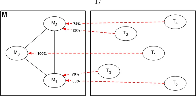
T4 T2 T3 T1 T5 M3 M1 M2 100% 26% 74% 70% 30%Figure 3.3: System view of the solution space
100 90 80 70 60 50 40 30 20 10 0
t1 t2 t3 ... ta tb tc ... tm tn
100 90 80 70 60 50 40 30 20 10 0
t1 t2 t3 ... ta tb tc ... tm tn
Time Time
Capacity % C1 Capacity % C2
T3 (r3x31 = 70% from 0 to tm)
T5 (r5x51 = 30% from ta to tn)
T4 (r4x42 = 74% from 0 to tm) T2
[image:25.612.151.488.273.408.2](r2x22 = 26% from t3 to tn)
Figure 3.4: Per-machine view of the solution space
We propose using a resource reservation system to solve the problem in two steps:
1. Assign each processing unitTito one machineMj.
2. Reserve a certain amount ofMj’s resourcerijforTi’s execution during its existence
in-terval.
Figures3.3and3.4 show a system view and a per-machine view of this solution space. Each resource reservation is of the form(ri, xijt, [Tstarti,Tendi]), where
• ridenotes the amount of resource that is reserved for streaming applicationi;
• xijt∈ {0,1}indicates whether streamiis assigned to machinejduring timet;
• [Tstarti,Tendi]is the time interval during which streaming applicationipersists (requiring
G
C1 C2
Input 1 Input 2 Input 3
G2 G1
T1 T2
T3
T4
T5
Output 1 Output 2
(a) problem example
T1 T2
T5
T3
M2 M3
M1
T4
q3 q5
q1 q2
q4
Input 1 Input 2 Input 3
[image:26.612.114.539.68.262.2](b) possible solution
Figure 3.5: Example of a mapping problem and a possible solution
Now we take a step back to see how to solve the overall mapping and scheduling problem:
1. Map streaming applications to machines.
(a) Assign each streaming application to a machine.
(b) Reserve a certain amount of that machine’s resource for that streaming application.
2. Locally schedule the executions of the streaming applications assigned to each machine.
Figure3.5(a) is our original pair of streaming applications, and Figure3.5(b) shows a possible mapping for this problem. TasksT1 andT2 are mapped to machine M1, and they each get a certain percentage ofM1’s resource reserved for their computations; TaskT3 is mapped to machineM3, and gets 100% ofM3’s resource; TasksT4 andT5 are mapped to machineM2, and each gets a certain percentage ofM2’s resource. Each machine has one queue for each task located on it, to receive that task’s inputs. At runtime, the machines make scheduling decisions about these queues based on several parameters, one of which could be the reservation amount for the corresponding task. The runtime scheduling step is described by Khorlin [17] in great detail.
Our focus is on the first step: mapping tasks to machines and making one reservation for each streaming application. We investigate a simpler version of the problem, where each streaming application consists of a single processing unit instead of a graph of interacting processing units and all streaming applications have the same existence interval. We propose the following problem formulation:
Let there beNstreaming applications, each with a concave utility functionUi(ri),i∈[1, N],
andMmachines, each with resource capacityCj,j∈[1, M]. In our system, we assume that
The objective is to determine the allocation of resources,ri(the amount of resource assigned to streamiduringi’s existence interval) andxij(a zero or one value indicating whether machine
j’s resource is allocated to streami), that maximizes the total utility:
max PN
i=1Ui(ri)
subject to PN
i=1rixij≤Cj for all j∈M ri≥0 for all i∈N
xij∈ {0,1} for all i∈N, j∈M.
3.4
Hardness Proof
We can prove the NP-completeness of our problem by reduction from the Multiple Knapsack Problem (MKP). The MKP involves a set of M bins with capacities C1. . . CM and a set of N
items with weightsw1. . . wN and valuesv1. . . vN. The objective is to find a feasible set of bin
assignments xij = {0,1} (xij = 1 if item i is assigned to binj) that maximizes the sum of
values of the items assigned to the bins. That is,
max PN
i=1
PM
j=1vixij
subject to PN
i=1wixij≤Cj for all j∈M xij∈ {0,1} for all i∈N, j∈M
PM
j=1xij≤1 for all i∈N.
Theorem 1 Our formulation of the resource allocation problem is NP-complete.
Proof Given any instance of the MKP {Cj,j∈[1, M]and(wi, vi),i∈[1, N]}, we can construct
an instance of our problem as follows: Let there beMmachines with capacitiesC1. . . CMandN
tasks, all with the same existence interval[t0, tk]and each with a constant utility function if the
resource assigned to it has value at leastwi,i.e.,Ui(PMj=1rjxij)=vi forri ≥wi. Thus, theM
machines correspond to theMbins, and theNtasks correspond to theNitems. For each task, the resource threshold valueri≥wi corresponds to the weight of the item, and the constant
utilityUi(PMj=1rjxij)=vicorresponds to the value of the item. By assuming that all streaming
applications have the same existence interval, we eliminate the time dimension, soxijt is the
assigned to bin/machinej. Under this setup, an optimal solution to our problem must assign at mostri = wi resource to streaming application i. Thus, the optimization problem can be
formulated as follows:
max PN
i=1
PM
j=1vixij
subject to PN
i=1wixij≤Cj for all j∈M xij∈ {0,1} for all i∈N, j∈M
PM
j=1xij≤1 for all i∈N.
We can therefore convert any instance of the MKP to an instance of our problem. If we can solve any instance of our problem in polynomial time, then we can solve any instance of the MKP in polynomial time. Since the MKP is known to be NP-complete, our problem is also NP-complete.
Chapter 4
Market-Based Heuristics
In this chapter, we present two heuristics for building the resource reservation systems using the competitive market concept from microeconomics. Both heuristics need to determine the best allocation of a machine’s resource to streams, which is equivalent to solving the following optimization problem:
max PN
i=1Ui(ri)
subject to PN
i=1rixi≤PMj=1Cj
ri ≥0 for all i∈N
xi∈ {0,1} for all i∈N, j∈M, t∈T .
This is equivalent to:
min −PN
i=1Ui(ri)
subject to PN
i=1rixi≤PMj=1Cj
ri ≥0 for all i∈N;
xi∈ {0,1} for all i∈N, j∈M, t∈T .
Since the objective functionPN
i=1Ui(ri)is concave and the constraints are linear, the problem
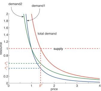
is a convex optimization problem and can be solved using convex optimization techniques. To avoid requiring each consumer to reveal its utility function to a centralized solver, we design a distributed method to solve the problem by using the market mechanism to solve its dual—the pricing problem. The pricing problem can be formulated as follows: There is a single market for resource with one supplier (the machine) andN consumers (the streaming applications). The supplier has an inelastic supply functionS =capacity. Each consumer has a continuous concave utility functionUi(r )=bir
1−ai
0
1
2
3
4
0
0.2
0.8
1
1.2
1.4
1.6
1.8
2
price
resource
demand1
demand2
total demand
p*
r
1*
r
2*
[image:30.612.157.495.80.386.2]supply
Figure 4.1: Demand, supply and optimal allocations
The supplier and the consumers interact with each other and participate in the price-adjustment process of the market:
1. The market sets an initial price.
2. While supply is not equal to total demand:
(a) Each consumer reacts to price and adjusts its optimal consumption level by equating its marginal utility and the current market price; that is, it setsUi0(r )=r−ai=price.
(b) The supplier reacts to demand and updates the market price according to the excess demand.
The equilibrium pricep∗is the price at which the total demand is equal to supply. At this
equilibrium price each consumer has a corresponding demandri∗, which forms the solution to the resource allocation optimization problem.
According to general equilibrium theory in microeconomics, there exists a unique equilib-rium price for this convex optimization problem at which the market clears (total demand equals total supply) and achieves maximum social welfare (maxPN
i=1Ui(ri)). The convergence
property of the algorithm is also guaranteed [24].
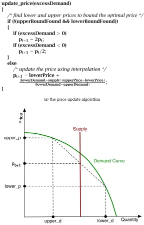
update_price(excessDemand) {
/* find lower and upper prices to bound the optimal price */
if (!(upperBoundFound && lowerBoundFound)) {
if (excessDemand>0) pt+1=2pt;
if (excessDemand<0) pt+1=pt/2;
} else
/* update the price using interpolation */
pt+1=lowerPrice+
(lowerDemand−supply)(upperPrice−lowerPrice)
(lowerDemand−upperDemand) ;
}
(a) the price update algorithm
upper_p
lower_p
lower_d upper_d
pt+1
Supply
Quantity
Price
Demand Curve
[image:32.612.180.468.163.612.2](b) pictorial description of the price update algorithm
4.1
Single Market Resource Reservation System
The first resource reservation system we present is a three step process:
1. Use a single market to determine the optimal allocation of the total system resource to each of the streams.
2. Use a variation of the First Fit Decreasing Utility heuristic to assign tasks to machines according to the optimal allocation.
3. Locally optimize the resource allocation to streams assigned to each machine.
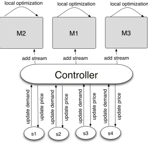
Figure4.3illustrates how the system works. There are three roles in the system:
1. Onecontroller for the entire system.
2. Onemachine agent for each machine.
3. Onestream agent for each streaming application.
M1
M2
M3
s2
local optimization
local optimization local optimization
Controller
update price
update demand
s3
update price
update demand
s1
update price
update demand
s4
update price
update demand
add stream add stream
[image:33.612.170.475.362.658.2]add stream
4.1.1
Algorithm
The algorithm has the following three steps:
1. controller: Assuming a virtual machineMv with capacity equal to the sum of the
capaci-ties of the machines in the systemP
Ci, use the local optimization algorithm to solve for
the optimal allocationr1. . . rn.
2. controller: Assign streaming applications to machines according to the best-fit-decrea-sing-value heuristic, where the size of each item isri and the value isU(ri)(details are
presented below).
3. eachmachine agent: Use the local optimization algorithm to determine the best alloca-tion of each machine’s resource to streaming applicaalloca-tions.
best-fit-decreasing-value In this step, streaming applications are assigned to machines based on the optimal allocation found in the previous step. The heuristic we use is a modified version of the best-fit-decreasing-value heuristic commonly used in the bin-packing problem. Given the allocationR =(r1∗. . . rN∗)and the corresponding utilitiesU =(U1(r1) . . . UN(rN)), do the
following:
1. Sort the tasks in decreasing order of utility.
2. Apply the best-fit-decreasing-value heuristic to assign these sorted tasks to machines.
(a) If the next taskTkcan be assigned to a machine according to its optimal allocation rk∗, do so.
(b) Otherwise, ifTkcan not be assigned to any machine according to the optimal
alloca-tion (∀j:rk∗≥remaining_Cj), put it in the set{RT}.
3. Assign the tasks in the set{RT}to machines using the best-fit-decreasing-value heuris-tic, regardless of the fact that the sizes of streaming applications are greater than the remaining capacities on the machines.
4.1.2
Lower Bound Analysis
We prove that, in the worst case, the solution found by our heuristic is a 2-approximation.
Theorem 2 Let U=P
Ui(ri)be the total utility achieved by our solution and Uopt be the total
utility achieved by the optimal allocation; thenU≥ 1
Proof Recall that our heuristic has three main steps: (1) run the local optimization algorithm on the virtual machine; (2) assign tasks to machines according to the resultingri; and (3) run
the local optimization algorithm on each machine. The first step solves the underlying convex optimization problem exactly and finds the optimal allocation of resources to tasks assuming all machine resources are gathered into one virtual machine. Thus the total utility achieved on the first step,U, serves as an upper bound on the optimal solution: U≥Uopt. If we can show
thatU≥ 12U, the proof is complete.
There are two substeps in the second step: (2a) assign tasks to machines according to ri∗
with the constraintri∗≤remaining_Cj; and (2b) assign remaining tasks to machines according
to ri∗ without the constraint ri∗ ≤ remaining_Cj. We now prove that, after (2a), the sum of
utilities of the assigned tasks is at least 12U.
Recall that each task has a valueUi(ri∗)and a sizer
∗
i . (2a) first arranges tasks in
decreas-ing order of valueUi(ri∗), then assigns the largest-valued task to a machine unless it doesn’t
fit within the remaining capacity of any machine. Let W1. . . Wj be the wasted space on the
machines after (2a). Let LT be the set of leftover tasks that can’t be assigned to a machine according to their sizesri∗. Then
W =XWj = X
i∈{LT}
ri.
We assumed that machine capacities were much larger than any individual task’s resource requirement, thus
maxr∗
i <minCj.
When no remaining task can be assigned to any machine, we have:
maxWj<minrk∗
Wj< rk
W M <
W |LT |
In the worst case, those M tasks are the ones with the(M+1)st, (M+2)nd, …,(2M)th
highest values, and the sum of their values is less than or equal to the combined value of tasks 1. . . M:
2M X
i=M+1
Ui(ri∗)≤ M X
i=1
Ui(ri∗)
2M X
i=M+1
Ui(ri∗)≤ 1
2U.
Therefore, after (2a), the total utility realized by the tasks assigned to the machines is more than half of the optimal. It is apparent that the remaining steps never decrease the total utility: step (2b) adds remaining tasks to machines, and step (3) does a local optimization on each machine to re-balance the resource allocations to the tasks on that machine and maximize the total utilities. That is, if the original allocation (r∗
i to tasks assigned during (2a), and 0 to tasks
assigned during (2b)) is optimal, then it is kept, otherwise the reallocation achieves higher total utility. Therefore, the total utility achieved by our heuristic is at least half of the optimal. 2
From the proof, it is apparent that the 12 lower bound is not tight. This conjecture is con-firmed by experiment and simulation, as described in Chapter5.
4.2
Multiple Market Resource Reservation System
The second resource reservation system we present models the system as multiple markets, one for each machine resource. This is analogous to the concept of multiple markets for sub-stitutable goods in microeconomics theory. Consumers/streaming applications can choose to purchase goods/resources from different markets based on the price information available to them. Under the assumption that streaming applications can’t split (each has to be pinned to one machine), the necessary condition for this M-commodity market to reach equilibrium is that theNstreaming applications can be partitioned intoM subsets, such that:
1. Ui0(xia)=Uj0(xjb), for alli, j∈[1, N]
2. Pricea=Priceb, for alla, b∈[1, M]
3. PN
i=1xia=Ca, for alla∈[1, M]
M1
M2
M3
pairwise comparison
stream movement
pairwise comparison
stream movement
pairwise comparison
stream movement
s1
s2
s3
s4
local optimization
[image:37.612.154.496.73.347.2]local optimization
local optimization
Figure 4.4: System view of the multiple-market method
Initially, each streaming application is assigned to one market (randomly or based on loca-tion). When all markets reach equilibrium, streaming applications from higher priced machines have incentives to move to lower priced machines. We enforce restrictions on when a stream-ing application may move from one machine to another: a move is allowed if and only if it increases the sum of the total utilities of the source and destination machines (theirpair-total utility). Each step of this process involves a pair of machines attempting to move one streaming application from one to the other and comparing the pair-total utilities before and after this attempt. This is an iterative monotonic process that increases (or leaves constant) the total utility at each step and terminates when no streaming applications can be moved from one ma-chine to another to increase the pair-total utility. Figure4.4illustrates how the system works. There are two roles in the system:
1. Onemachine agent for each machine.
2. Onestream agent for each streaming application.
The algorithm is as follows:
2. While there is at least one pair of streams in the system whose locations can be swapped to increase the total utility:
(a) Eachmachine agent runs the local optimization algorithm to find the equilibrium pricepj∗.
(b) machine agentscommunicate in pairwise fashion to move streams from one to an-other if the moves increase their pair-total utilities.
4.3
Summary
In this chapter, we have described two market-based heuristics for building resource reserva-tion systems.
The single-market heuristic uses a single market to determine the optimal allocation of total resources to each streaming application, and then uses engineering heuristic NFDV to assign streaming applications to each machine based on the optimal allocation. It has provably polynomial running time and a 12 lower bound on performance. We conjecture that this lower bound is loose (i.e., the real performance is much better than this lower bound).
However, although most of the computation in the single-market heuristic is done by the individual stream agents and machine agents, all the price and demand information needs to be exchanged between the centralized controller and the agents. Therefore, the communications overhead is large and the system does not scale well.
Chapter 5
Simulations
We evaluate the performances of the two heuristics developed in Chapter4through simulation. In the experiments, we assume that all streaming applications have utility functions of the form
Ui(ri)=bi
ri(1−ai)
(1−ai),ai ∈(0,1),bi∈(0,∞). We choose this particular class of functions because
it captures/approximates many concave functions that are typically used as utility functions [25]. To evaluate performance, we compare the total utility achieved by our heuristics with two metrics:
1. Upper bound U: the maximum total utility achieved assuming streams can split.
2. Base bound U: the total utility achieved by the naïve balanced-streamsheuristic, which assigns streams to balance the number of streams per machine.
In most of the figures below, we compare the performances of our heuristics and the balanced-streams heuristic by plotting the normalized performance gap (NPG)for each. The NPG for a heuristic is calculated as U−UU, whereU is the total utility achieved by the heuristic andUis the performance upper bound. Thus, the NPG is a number between 0 and 1; the smaller the NPG, the better the performance.
5.1
A Motivating Example
The balanced-streams heuristic has a randomness factor in its performance. That is, for N
streaming applications andM machines, it hasMN possible assignments, each occurring with
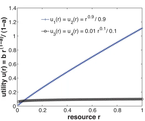
equal probability but resulting in different performance. We first use a motivating example to show that, in some cases, the naïve approach achieves arbitrarily bad performance where our heuristics each achieve near-optimal performance.
Suppose there are two machines, each with unit capacity C1 =C2 =1, and four streaming applicationsT1. . . T4, each with utility functionUi(ri)=bi
ri(1−ai)
0 0.2 0.4 0.6 0.8 1 0
0.2 0.4 0.6 0.8 1 1.2 1.4
resource r
utility u(r) = b r
(1−a)
/ (1−a)
u
1(r) = u2(r) = r 0.9
/ 0.9
u
3(r) = u4(r) = 0.01 r 0.1
[image:40.612.200.452.64.275.2]/ 0.1
Figure 5.1: Utility functions forT1. . . T4
b2=1,a3=a4=0.9, andb3=b4=0.01. ThusU1(r1)=U2(r2)= r
0.9
0.9 andU3(r3)=U4(r4)= 0.01r00..11 as shown in Figure5.1.
The balanced-streams heuristic has six possible assignments with equal probabilities. It has 13 probability of assigning T1 and T2 to the same machine, which results in allocations of r1 = r2 = r3 = r4 = 0.5 and total utility of U = 0.5953+0.5953+0.0933+0.0933 = 1.3772=0.59Uopt. Our market-based heuristics always assignT1andT2to different machines, resulting in allocations of r1 = r2 = 0.994 and r3 = r4 = 0.006 and total utility of U = 1.105+1.105+0.06+0.06=2.33=Uopt. Thus, the total utility achieved by the naïve
balanced-streams heuristic is only 1.23772.33 =59% of that achieved by our market-based heuristics for this example setup.
5.2
Heavy-tail Distribution
The stream processing applications follow a heavy-tail distribution if, under the optimal allo-cation on the virtual machine, many streams have small alloallo-cations, a few streams have large allocations, and very few fall in between. This distribution is typical for flows on the Internet, and is known as the “elephants and mice” distribution.
To test the performances of our heuristics under this distribution, we run the following experiments. Assume there are 2 machines in the system, each with unit capacity, andN = {3,4,5,6,7,8,9}streaming applications each with a utility functionUi(ri)=bi
ri(1−ai)
(1−ai). LetMof
the streaming applications have the parametersa=0.1,b=1, andN−Mhave the parameters
a=0.9,b=0.01.
Under this experimental setup, the balanced-streams heuristic has MN different
assign-ments. To compare the performances of the heuristics, we compute the average performance of the balanced-streams heuristic. This is done by brute force:
1. Run the heuristic under each of the possible assignments.
2. Compute the average utilities achieved by all possible assignments.
As shown in Figure5.2, the average performance of the balanced-streams heuristic stays at 85% of optimal, while both of our heuristics perform near 100% of optimal. The fully-decentralized multiple-market heuristic performs just as well as the single-market heuristic.
2 3 4 5 6 7 8 9
−0.1 0 0.1 0.2 0.3 0.4 0.5 0.6
number of streams
performance gap
[image:41.612.206.445.486.675.2]balanced−streams single−market multiple−market
5.3
Uniform Distribution
In this section, we analyze how different factors affect the performances of the three heuristics when the streaming applications follow a uniform distribution.
5.3.1
Comparison Among the Three Heuristics
To compare the performances of the three heuristics under a uniform stream distribution, we use the following experimental setup:
GenerateNstreaming applications, each with a utility functionUi(ri)=bi
ri(1−ai)
(1−ai), withai∈ (0.2,0.3)andbi∈(0,1)chosen randomly. GenerateMmachines, each with capacity 1.
Figure5.3shows the performances of the three heuristics with 7, 25, 42 and 111 machines in the system.
0 50 100 150 200 250 300
0 0.05 0.1 0.15 0.2 0.25 0.3
number of streams
performance gap
balanced−streams single−market multiple−market
(a) 7 machines
20 40 60 80 100 120 140 160 180
0 0.05 0.1 0.15 0.2 0.25 0.3 0.35 0.4
number of streams
performance gap
balanced−streams single−market multiple−market
(b) 25 machines
0 50 100 150 200 250
0 0.05 0.1 0.15 0.2 0.25 0.3 0.35
number of streams
performance gap
balanced−streams single−market multiple−market
(c) 42 machines
1000 150 200 250 300 350 400 450
0.05 0.1 0.15 0.2 0.25 0.3 0.35
number of streams
performance gap
balanced−streams single−market multiple−market
[image:42.612.112.537.309.687.2](d) 111 machines
The following observations are based on the simulation results:
1. The performances of our two market-based heuristics approach optimal quickly as the number of streaming applications increases.
2. The balanced-streams heuristic performs significantly worse than our market-based heu-ristics in all cases.
3. The performance gap for the balanced-streams heuristic decreases as the number of streams increases, but doesn’t converge to optimal (for up to 500 streams in the system), staying from 1% to 10% below optimal.
4. The more machines in the system, the larger the performance gap for the balanced-streams heuristic, and the slower the convergence of the two market-based heuristics.
5.3.2
The Effect of Number of Machines on Performance
To see how the number of machines affects the performance for each heuristic, we generate one plot for each heuristic showing the performances of that heuristic with various numbers of machines.
We use the same setup as the one in the previous section: N streaming applications, each with a utility functionUi(ri)=bir
(1−ai) i
(1−ai), withai ∈(0.2,0.3)andbi∈(0,1)chosen randomly; M machines, each with capacity 1. The following observations are based on the simulation results shown in Figure5.4:
1. For each fixed number of streaming applications in the system, the performance gap for the naïve balanced-streams heuristic increases as the number of machines increases.
2. Initially, for each fixed number of streaming applications in the system, the performance gaps for the two market-based heuristics increase as the number of machines increases; however, with increasing numbers of streaming applications, the performance gaps for all heuristics quickly converge to zero.
3. The fully-decentralized multiple-market heuristic performs almost as well as the single-market heuristic.
0 100 200 300 400 500 0 0.05 0.1 0.15 0.2 0.25 0.3 0.35 0.4
number of streams
performance gap
7 machines 25 machines 42 machines 111 machines
(a) balanced-streams heuristic
0 100 200 300 400 500
0 0.05 0.1 0.15 0.2 0.25 0.3 0.35 0.4
number of streams
performance gap
7 machines 25 machines 42 machines 111 machines
(b) single-market heuristic
0 100 200 300 400 500
0 0.05 0.1 0.15 0.2 0.25 0.3 0.35 0.4
number of streams
performance gap
7 machines 25 machines 42 machines 111 machines
[image:44.612.119.537.67.441.2](c) multiple-market heuristic
Figure 5.4: The effect of number of machines on heuristic performance
The valueU−Uhas two components:
1. The gap between the upper bound and the optimal value.
2. The gap between the optimal value and the heuristic result.
The first component is called theduality gap. It is the value forgone because of the ‘indivisible’ nature of the problem, and is irrelevant to the goodness of the heuristic.
0 2 4 6 8 10 0 0.05 0.1 0.15 0.2 0.25 0.3
number of streams per machine
performance gap
balanced−streams single−market multiple−market
(a) 7 machines
0 2 4 6 8 10
0 0.05 0.1 0.15 0.2 0.25 0.3 0.35 0.4
number of streams per machine
performance gap
balanced−streams single−market multiple−market
(b) 25 machines
1 2 3 4 5 6
0 0.05 0.1 0.15 0.2 0.25 0.3 0.35
number of streams per machine
performance gap
balanced−streams single−market multiple−market
[image:45.612.115.537.66.455.2](c) 42 machines
Figure 5.5: The effect of streams-to-machine-ratio on performance, by number of machines
0 2 4 6 8 10 0
0.05 0.1 0.15 0.2 0.25 0.3 0.35 0.4
number of streams per machine
performance gap
7 machines 25 machines 42 machines
(a) balanced-streams heuristic
1 2 3 4 5 6 7
0 0.05 0.1 0.15 0.2 0.25 0.3 0.35 0.4
number of streams per machine
performance gap
7 machines 25 machines 42 machines
(b) single-market heuristic
0 2 4 6 8 10
0 0.05 0.1 0.15 0.2 0.25 0.3 0.35 0.4
number of streams per machine
performance gap
7 machines 25 machines 42 machines
[image:46.612.118.540.198.574.2](c) multiple-market heuristic
5.3.3
The Effect of Total System Resource on Performance
To study how the total system resource affects the performance, we run the heuristics with three different mean values for machine capacity: 1, 0.1, and 0.01. We use a setup similar to the one in the previous section: Nstreaming applications, each with a utility functionUi(ri)=bi
ri(1−ai)
(1−ai),
withai∈(0.2,0.3)andbi∈(0,1)chosen randomly.
Each plot in Figure5.7shows the performances of the three heuristics with a distinct CPU mean value in a system with 42 machines. Figure5.8has one plot per heuristic, which shows the heuristic’s performance under three CPU mean values with 42 machines in the system.
0 50 100 150 200 250
0 0.05 0.1 0.15 0.2 0.25 0.3
number of streams
performance gap
balanced−streams single−market multiple−market
(a) cpu mean = 1
40 60 80 100 120 140 160 180 200
0 0.05 0.1 0.15 0.2 0.25 0.3 0.35
number of streams
performance gap
balanced−streams single−market multiple−market
(b) cpu mean = 0.1
0 50 100 150 200 250
0 0.05 0.1 0.15 0.2 0.25 0.3 0.35
number of streams
performance gap
balanced−streams single−market multiple−market
(c) cpu mean = 0.01
0 50 100 150 200 250
0 0.05 0.1 0.15 0.2 0.25 0.3 0.35
number of streams
performance gap
balanced−streams single−market multiple−market
[image:47.612.112.538.277.658.2](d) cpu mean = 0.001
40 60 80 100 120 140 160 180 200 0 0.05 0.1 0.15 0.2 0.25 0.3 0.35
number of streams
performance gap
cpumean=1
cpu
mean=0.1
cpu
mean=0.01
cpumean=0.001
(a) balanced-streams heuristic
40 60 80 100 120 140 160 180 200
0 0.05 0.1 0.15 0.2 0.25 0.3 0.35 0.4
number of streams
performance gap cpu mean=1 cpu mean=0.1 cpu mean=0.01
cpumean=0.001
(b) single-market heuristic
40 60 80 100 120 140 160 180 200
0 0.05 0.1 0.15 0.2 0.25 0.3 0.35 0.4
number of streams
performance gap
cpumean=1
cpumean=0.1
cpumean=0.01
cpu
mean=0.001
[image:48.612.120.536.56.443.2](c) multiple-market heuristic
Figure 5.8: The effect of total system resource on performance, by heuristic (42 machines)
The following observations are based on these plots:
1. Balanced-streams heuristic:
(a) The performance gap is larger when the total system resource is smaller.
(b) The performance gap decreases as the number of streams increases, but never con-verges.
2. Single-market heuristic:
(a) The performance gap is larger when the total system resource is smaller.
3. Multiple-market heuristic:
(a) The performance gap is larger when the total resource is smaller.
(b) The performance gap decreases as the number of streams increases and eventually converges to zero. The smaller the total resource, the slower it converges.
(c) Performance is almost as good as that of the single-market heuristic.
One reason that the performance gap increases with decreasing amount of total resource is the larger duality gap. An intuitive explanation is: when the total resource is scarce (supply is low), while the demands from the streams remain the same, the market is more competitive. Under a more competitive market, it is more important that the streams get their ‘optimal’ allocations because a small perturbation will result in a large utility loss. The theory behind this intuition is that, when the total resource is less, the resource each stream gets is also less. Since each stream has a concave utility function with decreasing marginal utility with respect to resource, less resource results in larger marginal utility. Thus, the system is more sensitive to the fact that the resource is fragmented among a number of machines. Therefore, a smaller amount of total resource results in a larger marginal utility, which in turn results in a larger performance gap.
The decrease in performance gap with increasing number of streaming applications is due to the decreasing duality gap; the more streaming applications in the system, the less resource each of them gets under the upper bound calculation. Thus, fewer of them fail to get their ‘optimal allocation’ when they are assigned to individual machines. This is similar to the bin packing example; given a set of fixed bins, it is easier to assign smaller balls to the bins than larger balls, so less bin volume is wasted by an inability to assign balls to bins.
5.3.4
The Effect of Utility Functions on Performance
Recall that each streaming application has a utility function of the form Ui(ri) = bi
ri(1−ai)
(1−ai),
ai ∈ (0,1), bi ∈ (0,∞). In this section, we study how the choices of a and b affect the
performances of the three heuristics.
5.3.4.1 Choice ofa
To test how parameteraaffects performance, we fix the range ofbto be(0,1)and the machine capacity to be 1, and run the heuristics with various ranges of a: (1)a ∈ (0.2,0.3); (2)a ∈ (0.2,0.5); (3)a∈(0.2,0.8); and (4)a∈(0.01,0.99). As shown in Figures5.9and5.10, when
0 50 100 150 200 250 0
0.05 0.1 0.15 0.2 0.25 0.3 0.35
number of streams
performance gap
a=(0.2,0.3) a=(0.2,0.5) a=(0.2,0.8) a=(0.01,0.99)
(a) balanced-streams heuristic
0 50 100 150 200 250
0 0.05 0.1 0.15 0.2 0.25 0.3 0.35
number of streams
performance gap
a=(0.2,0.3) a=(0.2,0.5) a=(0.2,0.8) a=(0.01,0.99)
(b) single-market heuristic
0 50 100 150 200 250
0 0.05 0.1 0.15 0.2 0.25 0.3 0.35
number of streams
performance gap
a=(0.2,0.3) a=(0.2,0.5) a=(0.