Overlapping Coalition Formation for Efficient Data Fusion in Multi Sensor Networks

Overlapping Coalition Formation for Efficient Data Fusion in Multi-Sensor

Networks

Viet Dung Dang, Rajdeep K. Dash, Alex Rogers and Nicholas R. Jennings

Southampton, SO17 1BJ UK Email:{vdd,rkd02r,acr,nrj}@ecs.soton.ac.uk

Abstract

This paper develops new algorithms for coalition formation within multi-sensor networks tasked with performing wide-area surveillance. Specifically, we cast this application as an instance of coalition formation, with overlapping coali-tions. We show that within this application area sub-additive coalition valuations are typical, and we thus use this struc-tural property of the problem to derive two novel algorithms (an approximate greedy one that operates in polynomial time and has a calculated bound to the optimum, and an optimal branch-and-bound one) to find the optimal coalition structure in this instance. We empirically evaluate the performance of these algorithms within a generic model of a multi-sensor net-work performing wide area surveillance. These results show that the polynomial algorithm typically generated solutions much closer to the optimal than the theoretical bound, and prove the effectiveness of our pruning procedure.

Introduction

Coalition formation (CF) is the coming together of a num-ber of distinct, autonomous agents in order to increase their individual gains by collaborating. This is an important form of interaction in multi-agent systems because many appli-cations require independent agents to come together for a short while to solve a specific task and disband once it is complete. As such, it has recently been advocated for task allocation scenarios where groups of agents derive a certain value (and/or cost) from tasks being performed in the coali-tion (Shehory & Kraus 1998). Building on this, in this pa-per, we apply CF to one such scenario, namely wide-area surveillance by autonomous sensor networks (e.g. perform-ing monitorperform-ing and intruder detection in areas of high se-curity). This is an important application that has received renewed interest in recent years, and a key question within this field, is how to coordinate multiple sensors in order to focus their attention onto areas of interest, whilst balancing the need for both coverage and precision. Thus the problem can naturally be modelled as one of CF since a number of groups of sensors need to be formed to focus on particular targets of interest, these groupings combine their resources for the group’s benefit and then they disband when the target is no longer present or a more important one appears.

Copyright c° 2006, American Association for Artificial Intelli-gence (www.aaai.org). All rights reserved.

However in order to apply CF within this domain, we need to extend the current state of the art. Specifically, to date, much of the research within this area has assumed non-overlapping coalitions in which agents are members of at most one coalition (see section Related Work for more de-tails). Now, in the multi-sensor networks that we consider, this assumption no longer holds. Since, the sensors can track multiple targets simultaneously, multiple overlapping coali-tions can be formed. Thus, against this background, this paper advances the state of the art in the following ways: • We cast the problem of sensor coordination for

wide-area surveillance as a coalition formation process, and show that, in general, this results in a coalition formation problem in which multiple coalitions may overlap and in which the coalition’s values are typically sub-additive. • We develop two novel algorithms to calculate the optimal

coalition structure when faced with overlapping coalitions and sub-additive coalitional values. The first is a polyno-mial time approximate algorithm that uses a greedy tech-nique and has a calculated bound from the optimum (Cor-men, Leiserson, & Rivest 1990). The second is an op-timal algorithm based on a branch-and-bound technique (Land & Doig 1960). We evaluate the performance of these algorithms in a generic setting, and show that the typical performance of the polynomial algorithm is typi-cally much better then the calculated bound. In addition, we show that the optimal branch-and-bound algorithm is able to effectively prune the search space.

The rest of the paper is organised as follows. In the next section we describe the wide-area sensing scenario that mo-tivates this work. Following this, we present our two al-gorithms for finding the optimal coalition structure in our overlapping coalition scenario. We empirically assess the performance of these algorithms in the following section, and finally, we conclude and discuss future work.

The Coalition Model

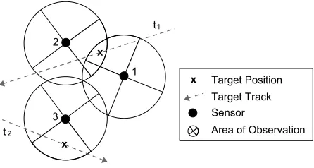
Figure 1: An example sensor network in which three sensors (1,2 and 3) track the position of two targets (t1andt2) that

pass through their field of view (indicated in bold).

the state it is in. Whensi= 0, the sensoriis the ‘sleep’ state (i.e. a state in which it is not sensing). The remainingKi−1 states are sensing states that indicate the directional capabil-ity of the sensor (i.e. an individual sensor can orientate its focus of attention into a number of distinct regions). Thus, depending on the sensing state that each sensor adopts, the sensor network as a whole may focus the attention of differ-ent combinations of sensors on to differdiffer-ent targets. Figure 1 shows a simple instantiation of such a sensor network. Here there are three sensors,I ={1,2,3} that are tracking two targets,T ={t1, t2}, within their field of view. The sensors

can either sleep or orientate their sensing in one of four di-rections. Since they have a fixed range, they can thus focus their attention within one of four sectors centered on the sen-sor itself (the active sector is shown in bold in the diagram). Now, a coalition in this scenario, is a group of sen-sors tracking a particular target (e.g. sensors 1 and 2 tracking target t1 in the example shown in figure 1). Let

visibility(i, si, tj)be a binary logical variable such that it istrueif targettjcan be observed by sensoriwhen in state si, andf alseotherwise. Then we can define a coalition as:

Definition 1 Coalition. A coalition is a tuple (C, tj) whereby C ⊆ I is a group of sensors such that∀i ∈ C, sensoriis in statesisuch thatvisibility(i, si, tj) =true.

Note that from the above definition, when an agent chooses to be in a particular state, it becomes a member of those coalitions that are responsible for tracking all the targets that are visible in that state, and thus, the sensor may be a mem-ber of several overlapping coalitions (this would occur in our example if another target fell within the active sensing sectors of both sensor 1 and 2).

Definition 2 Overlapping Coalitions. Two coalitions

(C, tj)and(D, tl)are overlapping ifC∩D6=∅

Now, each coalition(C, tj)has a valuev(C, tj)that rep-resents the value of having a number of sensors tracking a target (we discuss in the next section how this value is cal-culated). In addition, each sensor incurs costs depending on the sensing state that it has adopted. For example, the cost maybe zero when the sensor is turned on and non-zero otherwise. Moreover, in this paper, we are interested in the system welfare as it is an effective indication of the system’s

performance, especially in cooperative environments. Thus, the optimal coalition structure generation problem is to find a set of coalitions CS∗ _{= {(C}

1, t1), . . . ,(Cm, tm)} such that the system welfare is maximised:

CS∗= arg max

CS∈Γ(I,T) 

 X

tj∈T

v(Cj, tj)−

X

i∈I ci



 (1)

where Γ(I, T)is the set of all possible coalition structures given the targets and the agents. Note that unlike the stan-dard coalition model, in our formalism we can not simply in-corporate the costs into the coalition values. Doing so would incur multiple counting of the costs, since whilst there may bemcoalitions representing each target, there arensensors (and these sensors incur costs depending on their sensing state rather than the number of coalitions of which they are members).

Coalition Values

Now, since wide-area sensing is concerned with informa-tion gathering, it is natural to consider a coaliinforma-tion valua-tion funcvalua-tion based on the informavalua-tion content of observa-tions. In this case, the goal of the sensor network when co-ordinating the focus of individual sensors, is to obtain the maximum information from the environment. A common way to measure information in target tracking scenarios is to use Fisher information; a measure of the uncertainty of the estimated position of each target (Dash, Rogers, Reece, Roberts and Jennings 2005). Such a measure is attractive because when a number of sensors observe the same tar-get and then fuse their individual estimates, the information content of the fused estimate is simply given by the sum of the information content of the individual un-fused esti-mates. Thus, when the coalition value is represented as the information content of position estimates, the coalition val-ues are additive. For example, in figure 1 where both sensors 1 and 2 observe and fuse information about target 1, then v({1,2}, t1) =v({1}, t1) +v({2}, t1).

However, this additivity only applies when the individual estimates are independent. A more likely scenario within sensor networks is that these individual estimates are cor-related to some degree. This will typically occur either through the exchange and fusion of earlier position esti-mates, or alternatively, by sensors using shared assumptions (such as a common model of the target’s motion). Now, when these estimates are correlated, the coalition values be-come sub-additive (Reece and Roberts 2005). That is, due to the correlation, the fused estimate contains less informa-tion than the sum of the individual estimates, and thus, in our example,v({1,2}, t1)< v({1}, t1) +v({2}, t1).

Thus, in this paper, we focus on coalition values that obey the following two conditions:

• Monotonicity:v(C, tj)≤v(D, tj)ifC⊆D

This ensures that adding new members to a coalition can never reduce its value. In our case, this implies that ob-taining observations from more sensors about a target can-not decrease the coalition value.

• Sub-additivity:v(C∪D, tj)≤v(C, tj) +v(D, tj) This implies that if two different groups of sensors track a certain targettj, then the sum of the value each derives is never less than if the union of the two groups perform it. In our scenario, suppose a group of sensorsCtracks a targettj. Now suppose another group of sensorsDtrack the same target. Then the sum of the value of these two exclusive events cannot be less than if all the members of CandDjoined to track the same target. Sub-additivity intuitively occurs whenC∩D 6=∅or due to the dimin-ishing returns each new member brings to a coalition.

Sensor Costs

As described above, the costs of the sensors are calculated separately from the coalition value. In the case of simple sensors that incur a fixed cost dependent on their statesi, we can model the cost as:

ci=

½ _0if si= 0 costiotherwise

In more complex settings, the sensor cost may also reflect the additional costs incurred when changing from one sens-ing state to another (e.g. the cost of changsens-ing its orienta-tion to track another set of targets), or reflect the fact that in battery power devices the cost of sensing may depend on the state of charge of the battery. However, in this paper, we consider the simple cost structure since this issue has no impact on the performance of our coalition formation algo-rithms, which we now describe.

Coalition Formation Algorithms

In this section, we present our two coalition formation al-gorithms. Specifically, we describe a fast polynomial, ap-proximate algorithm (that can produce a solution within a finite bound of the optimal), and then an optimal branch-and-bound algorithm.

The Polynomial Algorithm

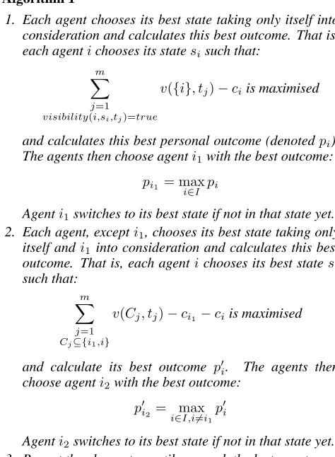
Algorithm 1 is a polynomial time algorithm that produces an approximation of the optimal solution (see figure 2). Basi-cally, it operates in a greedy manner. It first chooses the best action by a sensor (e.g. the action that brings the biggest value) (see step 1). In the second step, it chooses the best action of another sensor taking the first sensor into consid-eration. Then, in the third step, it chooses the best action of another sensor taking the first two sensors into consider-ation. The process then repeats until there is no sensor left. We can now analyse the algorithm to assess its properties.

Theorem 1.1 The complexity of algorithm 1 isO(n2m).

Algorithm 1

1. Each agent chooses its best state taking only itself into consideration and calculates this best outcome. That is, each agentichooses its statesisuch that:

m

X

j=1

visibility(i,si,tj)=true

v({i}, tj)−ciis maximised

and calculates this best personal outcome (denotedpi). The agents then choose agenti1with the best outcome:

pi₁= max i∈I pi

Agenti1switches to its best state if not in that state yet.

2. Each agent, excepti1, chooses its best state taking only

itself andi1into consideration and calculates this best

outcome. That is, each agentichooses its best statesi such that:

m

X

j=1

Cj⊆{i1,i}

v(Cj, tj)−ci₁−ciis maximised

and calculate its best outcome p′

i. The agents then choose agenti2with the best outcome:

p′i2= max_i∈I,i6=i 1

p′i

Agenti2switches to its best state if not in that state yet.

3. Repeat the above step until we reach the last agent.

Figure 2: The polynomial coalition formation algorithm.

PROOF. At each step, it requires to get throughO(n)sensors to find the best action of a sensor. For each sensor, we have to calculate the outcome for each state by summingO(m)

coalition values together. As there arensteps, the complex-ity isO(n2m).¤

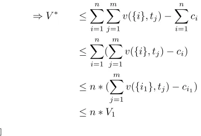
Theorem 1.2 The solution of algorithm 1 is within a bound nof the optimal. That is, given thatV1is the system welfare

of the solution of algorithm 1 andV∗the optimal solution:

V∗

V1

≤n

PROOF. Leths∗iini=1be the optimal state vector (that is, the

vector contains the states of all sensor agents). For 1 ≤ j≤m, letCj∗be the coalition of sensors that track targettj associated with the optimal solution. The optimal solution’s system welfareV∗then is:

V∗ =

m

X

j=1

v(Cj∗, tj)− n

X

i=1

ci

≤ m

X

j=1 X

i∈C∗

j

v({i}, tj)− n

X

i=1

⇒V∗ ≤ n

X

i=1

m

X

j=1

v({i}, tj)− n

X

i=1

ci

≤ n

X

i=1 (

m

X

j=1

v({i}, tj)−ci)

≤n∗(

m

X

j=1

v({i1}, tj)−ci₁)

≤n∗V1

¤

The Optimal Algorithm

The optimal algorithm is a branch-and-bound algorithm that finds the optimal solution. First, however, we define the con-cept of a weak state as it will be used in the algorithm.

Definition 3 A statesiof agentiis called a weak state iff agentiin statesidoes not see any target in its range.

Proposition 1 A state vectorhs1, s2, ..., sniis not optimal if there exists anisuch thatsiis a weak state.

PROOF. This is trivial due to the fact thatV(s1, s2, ..., sniis always less thanV(s1, ..., si−1,0, si+1, ..., sni(0 means the sleeping state).¤

We present the branch-and-bound algorithm in figure 4. This basically searches through the search space in a depth-first search manner, then uses a branch-and-bound technique to prune a subtree whenever possible. Specifically, if we reach a node and the upper bound value of all nodes that branch under that node is less than or equals the current best so-lution, we can prune the whole subtree under the node. The original best solution is the solution of the greedy algorithm, while the upper bound of the subtree is derived from the sub-additivity as detailed in figure 4. Also see figure 3 for an example search tree in casen = 3andki = 2, for all

1≤i≤n.

Now one of the main issues that affects the performance of Branch-and-Bound algorithms is choosing the tree struc-ture. To this end, we present a process for selecting the tree structure (which in this case is equivalent to an order-ing of the agents) with which the algorithm will likely prune the subtrees quickly (see figure 5). Basically, it contains 2 phases. In the first one, all agents with weak states are cho-sen first and ordered decreasingly according to the number of their weak states. The idea is to maximise the number of pruned subtrees early on (due to proposition 1). In the second phase, the remaining agents are ordered in a simi-lar way to the greedy algorithm (but in reverse). That is, it first chooses the worst action by a sensor. In the sec-ond step, it chooses the worst action of another sensor tak-ing the first sensor into consideration. Then, in the third step, it chooses the worst action of another sensor taking the first two sensors into consideration. The process then re-peats until there is no sensor left. In this way, the inequation V(S′)≥V(α1, α2, ..., αk) +P

n

i=k+1V(si)is more likely to happen asV(α1, α2, ..., αk)is likely to be small.

Figure 3: An example search tree withn= 3andki = 2, for all1≤i≤n.

Algorithm 2

1. Search allhs1, s2, ..., sniin a depth-first search manner. 2. Suppose the current best system welfare isV1(initially V1_{would be the system welfare generated by the greedy}

algorithm). IfV1 ≥Vu_,Vu_{is the upper bound of the} value of any solution in the subtreehα1, α2, ..., αki(i.e. hs1=α1, s2 =α2, ..., sk=αki), prune the whole sub-treehα1, α2, ..., αki. The upper bound is derived from sub-additivity property of the valuation function as fol-lows: for everysk+1, sk+2, .., sn:

V(α1, α2, ..., αk, sk+1, sk+2, ..., sn)

≤V(α1, α2, ..., αk,0,0, ...,0) + n

X

i=k+1

pi

Thus if we have V1 _{≥ V(α}

1, α2, ..., αk,0,0, ...,0) +

Pn

i=k+1pi, the whole sub-tree hα1, α2, ..., αkican be pruned safely.

3. If we reach a leaf node in the tree, calculate its valuation and update the current best solution.

Figure 4: The optimal coalition formation algorithm.

Experimental Results

This section outlines the experimental evaluation of our al-gorithms to see how they perform in reality. This is neces-sary because, for our polynomial algorithm, the theoretical analysis is in terms of worst-case, however, by doing an ex-perimental analysis we can have a clearer idea of the typi-cal performance; and for our optimal one, it is difficult to measure its effectiveness theoretically. Specifically, for the polynomial algorithm, we want to assess how close a typical solution is to the optimal compared to the worst-case bound, and for the optimal algorithm, we want to assess how effec-tively the search space is pruned. To this end, we next de-scribe the experimental setup in subsection, and then present the evaluation results for the polynomial and optimal algo-rithms separately.

Experimental Setup

Algorithm 3

1. Choose an agent with the biggest number of weak states. 2. Repeat step 1 until no agent with weak states is left. 3. For the remaining agents, carry out the following steps:

• Each agent chooses its worst state taking only itself into consideration and calculates this worst outcome. That is, each agentichooses its statesisuch that:

m

X

j=1

v({i}, tj)−ciis minimised

and calculates its worst outcome pi. The agents then choose agenti1with the worst outcome:

pi₁ = mini∈Ipi

• Each agent, except i1, chooses its worst state taking

only itself andi1into consideration and calculates this

worst outcome. That is, each agentichooses its worst statesisuch that:

m

X

j=1

Cj⊆{i1,i}

v(Cj, tj)−ci₁−ciis minimised

and calculates its worst outcome p′

i. The agents then choose agenti2with the worst outcome:

p′i₂ = mini∈I,i6=i1p

′

i

• Repeat the above step until we reach the last agent.

Figure 5: The tree structure selection process for the optimal coalition formation algorithm.

network described in figure 1. That is, we haven(ranging from 4 to 20 in the experiment) sensors, each with a fixed range and four distinct sensing states, randomly distributed within a unit area. Within this area arem(that has the same value asnin the experiment) targets, again randomly dis-tributed. We assign a random sensing cost on the interval

[0,1) to each sensor, and a random coalition value, again on the interval[0,1), to each coalition that contains a sin-gle sensor. We then use an iterative process to randomly assign the coalition values of all the larger coalition, whilst ensuring that these values satisfy our monotonicity and sub-additivity constraints. In this way, we calculate problem in-stances that are as general as possible, and thus, do not bias our results to a specific scenario.

Now, due to the demands of space, here we setnequal tom. Then for values of 4, 8, 12, 16 and 20 targets and sensors, we run the algorithms 200 times1 _{and record the}

bound from the optimal (for the polynomial algorithm) and the percentage of pruned space (for the optimal algorithm).

1_{An ANOVA test showed that 200 iterations is sufficient for} statistically significant results. Forα= 0.05_{, the p-value for the} null hypothesis is> 0.05_{in all the experiments with 5 samples.} This shows that there is not a significant difference between the mean values and thus validates the null hypothesis.

4 8 12 16 20

0 20 40 60 80 100

Number of Agents (n)

Percentage

Figure 6: Percentage of searches that return the optimal value in the case of the polynomial algorithm.

Number of Sensors

Mean Bound Std Dev and Targets

4 1.0028 0.024

8 1.0062 0.022

12 1.0071 0.023

16 1.0054 0.013

20 1.0078 0.012

Table 1: Polynomial algorithm – bound from the optimal.

The Polynomial Algorithm

The result for the polynomial algorithm is presented in ta-ble 1 and figure 6. As we can see from the tata-ble, all of the bounds are very close to 1. Specifically, the bound mean is always less than 1.01 and the standard deviation is always less than 0.03. This is close to the optimal and significantly lower than the theoretically proved bound which isn(i.e., 4 to 20 in this experiment). This suggests that in many prac-tical cases, our algorithm performs significantly better than the theoretical proved worst-case analysis. Moreover, from figure 6, we see that when the number of sensors and targets is small, the greedy algorithm generates the optimal solution a significant percentage of the time (i.e. greater than 80% whenn=m= 8). However, as the number of sensors and targets increase, the problem instances become more diffi-cult to solve, and thus, this percentage decreases.

The Optimal Algorithm

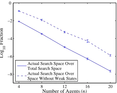
The result for the optimal algorithm is presented in figure 7. This logarithmic plot shows the degree to which the branch-and-bound algorithm is able to exploit the known structure of the problem (i.e. monotonicity and sub-additivity) in or-der to be able to prune the search space. Note that when n =m = 20, the algorithm needs to typically only search

10−8_{of the entire search space in order to calculate the}

4 8 12 16 20 −8

−6 −4 −2 0

Number of Agents (n)

Log

10

Fraction

Actual Search Space Over Total Search Space Actual Search Space Over Space Without Weak States

Figure 7: Comparison of various search spaces in the opti-mal algorithm.

Related Work

A number of algorithms have been developed for coalition formation, but in general these have not considered overlap-ping coalitions (Sandholm et al. 1999; Dang & Jennings 2004). However, the notion of overlapping coalitions was introduced by Shehory and Kraus in their seminal work on coalition formation for task allocation (Shehory & Kraus 1998; 1996). Here they developed a greedy algorithm for finding a solution to the overlapping coalitions problem that exhibited logarithmic bound. However, in contrast to our problem, they considered a specific block-world scenario in which the tasks had a precedence ordering and the agents had a capability vector (denoting the ability of the agents to perform tasks). As a result, the algorithm they develop is dissimilar to our polynomial algorithm. Moreover, they do not develop an optimal algorithm for the overlapping coali-tion formacoali-tion process.

The application of coalition formation techniques to dis-tributed sensor networks has also been investigated by a number of researchers. In (Sims, Goldman & Lesser 2003), a vehicle-tracking sensor network is modelled using disjoint coalitions formed via a negotiation process that results in a self-organising system. Similarly, in (Soh, Tsatsoulis & Se-vay 2003), negotiation techniques are employed in order to form coalitions that track a target. However, these works fo-cus on identifying and negotiating with potential coalition members since they operate in an incomplete information scenario where they are not aware about the existence and capabilities of other sensors. Our work on the other hand focuses on providing algorithms for the coalition formation process in a complete information environment.

Conclusions and Future Work

In this paper, we considered coalition formation for multi-sensor networks applied to wide-area surveillance. Specif-ically, we showed how this application leads to overlap-ping coalitions which exhibit sub-additivity and monotonic-ity, and we designed two novel coalition formation algo-rithms that exploit this particular structure. The first was

an approximate and polynomial algorithm, with complexity O(n2m), that exhibited a calculated bound from the optimal ofn. The second, which was optimal and based on a branch-and-bound heuristic, used a novel pruning procedure in or-der to reduce the number of searches required. We used em-pirical evaluations on randomly generated data-sets to show that the polynomial algorithm typically generated solutions much closer to the optimal than the theoretical bound, and to prove the effectiveness of our pruning procedure.

Future work will focus on employing these algorithms within dynamic environments where the values of the tions change with time, thereby causing the optimal coali-tion structure to vary. This will occur in our scenario as targets move in and out of the sensors’ range of observa-tion. We also plan to test these algorithms on real data from multi-sensor networks in order to further evaluate their per-formance in real-life scenarios.

Acknowledgement

This research was undertaken as part of the ARGUS II DARP. This is a collaborative project involving BAE SYSTEMS, QinetiQ, Rolls-Royce, Oxford University and Southampton University, and is funded by the industrial partners together with the EPSRC, MoD and DTI.

References

Cormen, T., Leiserson, C. and Rivest, R. 1990. Introduction to Algorithms. MIT Press.

Dang, V. D. and Jennings, N. R. 2004. Generating coalition structures with finite bound from the optimal guarantees. In Proc. 3rd Int. Conf. on Autonomous Agents and Multi-Agent Systems, 564–571.

Dash, R. K., Rogers, A., Reece, S., Roberts, S. and Jennings, N. R. 2005. Constrained bandwidth allocation in multi-sensor information fusion: A mechanism design approach. In Proc. 8th Int. Conf. on Information Fusion.

Land, A. H. and Doig, A. G. 1960. An automatic method for solving discrete programming problems. Econometrica 28:497– 520.

Lesser, V., Ortiz, C. and Tambe, M., eds. 2003. Distributed Sen-sor Networks: A multiagent perspective. Kluwer Publishing. Reece, S. and Roberts, S. 2005. Robust, low-bandwidth, multi-vehicle mapping. In Proc. 8th Int. Conf. on Information Fusion. Sandholm, T., Larson, K., Andersson, M., Shehory, O. and Tohme, F. 1999. Coalition structure generation with worst case guarantees. Artificial Intelligence 111(1-2):209–238.

Shehory, O. and Kraus, S. 1996. Formation of overlapping coali-tions for precedence-ordered task-execution among autonomous agents. In Proc. 2nd Int. Conf. on Multiagent Systems, 330–337. Shehory, O. and Kraus, S. 1998. Methods for task allocation via agent coalition formation. Artificial Intelligence 101(1–2):165– 200.