Bayesian modelling of music: algorithmic advances and experimental studies of shift invariant sparse coding

(1)

ePrints Soton

Copyright © and Moral Rights for this thesis are retained by the author and/or other

copyright owners. A copy can be downloaded for personal non-commercial

research or study, without prior permission or charge. This thesis cannot be

reproduced or quoted extensively from without first obtaining permission in writing

from the copyright holder/s. The content must not be changed in any way or sold

commercially in any format or medium without the formal permission of the

copyright holders.

When referring to this work, full bibliographic details including the author, title,

awarding institution and date of the thesis must be given e.g.

AUTHOR (year of submission) "Full thesis title", University of Southampton, name

of the University School or Department, PhD Thesis, pagination

(2)

Bayesian Modelling of Music:

Algorithmic Advances and

Experimental Studies of

Shift-Invariant Sparse Coding

Thesis submitted in partial fulfilment of the requirements of the University of London

for the Degree of Doctor of Philosophy

Thomas Blumensath

Submitted: October 2005 Corrections: January 2006

(3)

other people, published or otherwise, are fully acknowledged in accordance with the standard referencing practices of the discipline. I acknowledge the helpful guidance and support of my supervisor, Dr Mike Davies.

(4)

Abstract

In order to perform many signal processing tasks such as classification, pattern recognition and coding, it is helpful to specify a signal model in terms of meaningful signal structures. In general, designing such a model is complicated and for many signals it is not feasible to specify the ap-propriate structure. Adaptive models overcome this problem by learning structures from a set of signals. Such adaptive models need to be general enough, so that they can represent relevant structures. However, more general models often require additional constraints to guide the learning procedure.

In this thesis a sparse coding model is used to model time-series. Rele-vant features can often occur at arbitrary locations and the model has to be able to reflect this uncertainty, which is achieved using a shift-invariant sparse coding formulation. In order to learn model parameters, we use Bayesian statistical methods, however, analytic solutions to this learning problem are not available and approximations have to be introduced. In this thesis we study three approximations, one based on an analytical integral approximation and two based on Monte Carlo approximations. But even with these approximations, a solution to the learning problem is computationally too expensive for the applications under investigation. Therefore, we introduce further approximations by subset selection.

Music signals are highly structured time-series and offer an ideal testbed for the studied model. We show the emergence of note- and score-like fea-tures from a polyphonic piano recording and compare the results to those obtained with a different model suggested in the literature. Furthermore, we show that the model finds structures that can be assigned to an indi-vidual source in a mixture. This is shown with an example of a mixture containing guitar and vocal parts for which blind source separation can be performed based on the shift-invariant sparse coding model.

(5)

(6)

Acknowledgements

I am very grateful to have been given the opportunity to spend the last three years dedicated to the research which led to this thesis. This would not have been possible had I not received tremendous support from my family, friends and colleagues. I would like to thank my father first of all, as his support enabled me to fully concentrate on my work without financial worries. I would also like to thank the rest of my family for believing in me, even though they could not always fully grasp all the issues involved in my work.

Probably the most influential person during my time as a postgraduate student was my supervisor Dr Mike Davies. I have been extremely lucky to be working with a person who shared the same outlook on many scientific topics with me. Without his guidance I would not have been able to achieve even a fraction of what I have. I would like to thank him for the freedom I was given and the inspiring discussions we had even though these were often sparsely distributed. These discussions can be seen as the foundations of this thesis.

The Centre for Digital Music has been a fantastic place to study and work. It offered the perfect environment for research providing ample op-portunity to discuss research and learn from the experiences of a broad variety of persons with different backgrounds and ideas. Of all the re-searchers in the group, the greatest influence on my work had Samer Ab-dallah, whose thesis inspired me to follow the research which led to this thesis.

I also would like to thank Dan Ellis, who allowed me to spend two productive months during the Summer of 2004 in the Laboratory for the Recognition and Organisation of Sound and Audio at Columbia University in the City of New York. This stay was made possible by the generous support of the Royal Society of Engineering and the EPSRC Digital Music

(7)

From my university life before research, I would like to thank Iain Paterson-Stephens, who first introduced me to the world of digital sig-nal processing during my undergraduate years and who was the first to encourage me to study for a PhD.

Most of my gratitude must go to the most important person in my life, Rachel, who kept me sane and well dressed during the last three years. I appreciate the sacrifices she made for me and my studies during our lives in separate parts of the country. Rachel had more direct influence on my work, spending much of her valuable time reading through many of my papers and in particular this thesis to criticise my often ‘unconventional’ use of the English language. As the reader can verify, I have often ignored her advice.

(8)

List of Figures

3.1 Filtering effects and path in three dimensions . . . 60

5.1 Efficiency comparison of importance sampling method . . . 89

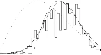
6.1 Comparison of note velocity histogram and modified Ray-leigh distribution . . . 95

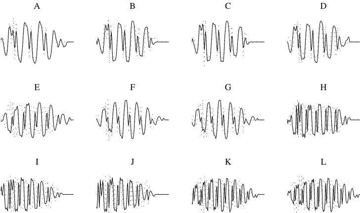
7.1 Notes used to generate test signal . . . 108

7.2 Features found with the Gibbs sampling method using a modified Rayleigh delta mixture prior . . . 110

7.3 Features found with the importance sampling method . . . 110

7.4 Learning performance for a specific feature . . . 111

7.5 Comparision of the correlation between learned features and original notes and the histogram of note occurrence . . 114

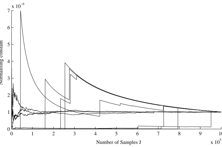
7.6 Convergence of the normalising constant estimate for the importance sampler . . . 116

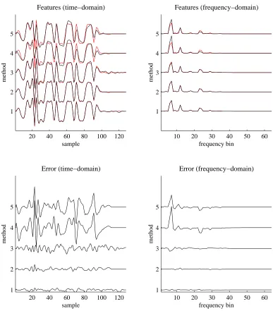
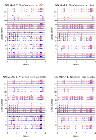
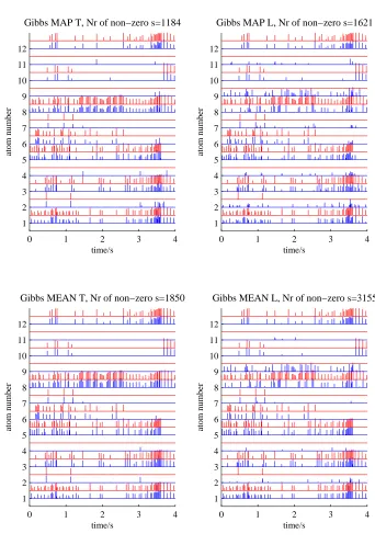
7.7 Comparision of true and learned representations using the Gibbs sampler with the modified Rayleigh/delta mixture prior . . . 120

7.8 Comparision of true and learned representations using the Gibbs sampler with the Gaussian/delta mixture prior . . . 121

7.9 Comparision of true and learned representations using the importance sampler . . . 122

7.10 Comparision of true and learned representations using the EM algorithm . . . 123

7.11 Features learned with the Gibbs sampler . . . 125

7.12 Features learned with the EM method . . . 126

7.13 Features learned with the importance sampler . . . 127

7.14 Comparision of spectra between the EM and the Gibbs methods . . . 128

8.1 Principal component analysis of piano notes . . . 134

(13)

8.3 The learned features . . . 138

8.4 Analysis of emerging score-like structure . . . 139

8.5 Transcription performance of different approaches . . . 145

8.6 True positives vs. false positives . . . 146

9.1 Time-domain waveforms of the dictionary learned using the time-domain method . . . 153

9.2 Log spectra of the dictionary learned using the time- and spectral-domain approach . . . 154

9.3 Approximation coefficients found with time-domain method 155 9.4 Approximation coefficients found with the spectral-domain method . . . 155

9.5 Representation of the notes from the Bagatelle . . . 156

9.6 Comparison of the waveform of a single piano note with some features learned using the time-domain method . . . 157

9.7 Comparison of the magnitude spectrum of a single piano note with the magnitude spectra of features learned using the time-domain method . . . 158

9.8 Activity of the five features modelling a single note . . . . 159

9.9 Comparison of the magnitude spectrum of two features learned using the spectral-domain method . . . 160

9.10 Activity of the two features modelling a single note . . . . 160

10.1 Analysis of emerging structures . . . 165

10.2 Distortion (in dB) for the separated sources . . . 166

10.3 Distortion (in dB) for the blindly separated sources . . . . 170 B.1 Efficiency of the different Gibbs sampler implementations . 210

(14)

List of Tables

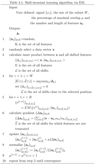
4.1 Shift-invariant learning algorithm via EM . . . 77

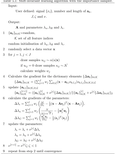
5.1 Shift-invariant learning algorithm with importance sampler 87 6.1 Shift-invariant learning algorithm with a Gibbs sampler . . 103

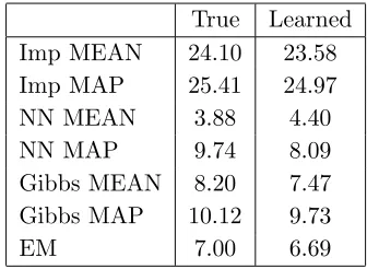
7.1 Correlation between the learned features and the original notes . . . 113

7.2 Model parameter estimation . . . 115

7.3 Reconstruction error . . . 118

7.4 Number of atoms . . . 124

8.1 Comparison of transcription performance . . . 143

8.2 Different sources of error encountered in the transcription . 148 10.1 Comparison between the features for clustering. . . 169

(15)

an feature

akl feature k at shift l

c term used to abbreviate equations d double atoms

f regularisation or error term

f n false negative error

f p false positive error

g regularisation or error term

i index of observations; also used as index of index, i.e. sni

j index of sample

k index of function in shift-invariant model

l index of function shift and with slight abuse of notation the amount of shift associated with this index

m index of sample in the observation vector x

n index of column in matrix A

p p=m+l

p(·) probability density function of a variable

r index of iteration in iterative algorithms and index in bridged transition sampler

s source vector or coefficient vector of length N

s∗ _{fixed point of an iterative algorithm}

u binary indicator variable of mixture prior

w weight in importance sampling algorithm x observation vector of lengthM

A mixing matrix or dictionary

(16)

F length of functions ak H Hessian

I number of all observations I identity matrix

I set of indices for all observations

J number of samples in Monte Carlo approximation

K number of all features

K set of indices for all features

L number of all shifts

L set of indices for all shifts

L1 L1 norm, P| · |

L0 L0 norm, number of nonzero values or numerosity

Lp Lp norm, (P| · |p)1/p

M length of observation vector x

N length of coefficient vector s

Nø number of non-zero s

N normal distribution

RB maximum number of annealing steps T temperature in annealing

W weighting matrix in IRLS

W maximum number of elements in subset

Z normalising constant

α parameter in α-stable distribution

∂·

∂A short for { ∂·

∂a_mn}mn, i.e. matrix of derivatives w.r.t. amn ǫ vector of observation noise

λ= λc

λǫ parameter relating sparseness to reconstruction error

λc function of prior variance

λu parameter of hyper-prior in mixture model λǫ inverse of error variance σ2ǫ

λmax maximum λ value

(17)

σ2

ǫ variance of a scalar random variable or of a vector random

variable with covariance matrix σ2

ǫI η location parameter in Rayleigh density

θ vector of model parameters

µ mean of Gaussian density

ν learning rate

τ prior variance

ψ λc+λR

Σǫ σǫ2I

∆ gradient

Σs covariance matrix for Gaussian prior

ø index of non-zero coefficients

k · k norm (L2 norm if not specified otherwise)

<_·> expectation, the density, if not specified, should be clear from the context

∼ is distributed as

ˆ_· approximated quantity

diag(_·) square matrix with the elements _·along the diagonal

(18)

Abreviations

BP basis pursuit

BSS blind source separation

dB deci Bell

EM expectation maximisation

FFT fast Fourier transform fn false negative

FOCUSS focal underdetermined system solver fp false positive

ICA independent component analysis

i.i.d independent and identically distributed IRLS iterative re-weighted least squares

MA moving average

MAP maximum a posteriori MCMC Markov chain Monte Carlo

MIDI musical instrument digital inteface

ML maximum likelihood

MP matching pursuit

OMP orthogonal matching pursuit

PCA principal component analysis ROC receiver operation curve

RVM relevance vector machine SAR signal to artefact ratio SDR signal to distortion ratio

SIR signal to interference ratio w.r.t. with respect to

(19)

“[...] we may consider the idea of building an induction machine. Placed in a simplified ‘world’ (for example, one of sequences of coloured counters) such a machine may through repetition ‘learn’, or even ‘formu-late’ laws of succession which hold in its ‘world’. [...]

In constructing an induction machine we, the architects of the ma-chine, must decide a priori what constitutes its ‘world’; what things are to be taken as similar or equal; and what kind of ‘laws’ we wish the ma-chine to be able to ‘discover’ in its ‘world’. In other words we build into the machine a framework determining what is relevant or interesting in its ‘world’: the machine will have its ‘inborn’ selection principles. The problem of similarity will have been solved for it by its makers who thus have interpreted the ‘world’ for the machine.”

(20)

Chapter 1 Introduction

In this thesis we study an ‘induction machine’ to use the term offered by Popper in the quote above. How can such an ‘induction machine’ ‘discover’ and ‘learn’ ‘laws’ of nature, how can it find structure in its ‘world’ and what ‘constraints’ do we, the designer of such a machine, have to impose? First, the ‘world’ of such a machine needs to be specified. In this thesis we do not deal with the coloured counters of Popper’s example but instead use music recordings. These signals have a great amount of structure and are, in fact, designed to contain such structures. However, this structure also shows unpredictable variation, for example the waves of sound pressure produced by a particular performance vary depending on many quantities of the instrument, the acoustics of the room, the temperature and the performer. Higher level structures such as timing and the acoustic energy of notes also vary between different performances. Our ‘induction machine’ must account for this variability which is done using probabilistic components and, in particular, Bayesian techniques.

Extracting information and structure from data seems a trivial exercise at first. Is it not easy for us to hear and understand spoken language even in noisy environments and is it not an effortless task to distinguish the face of your grandmother from most other faces? Only once we start to think about the computational processes required to achieve such tasks does it become clear how difficult these tasks are and what an extraordinary undertaking the human brain performs.

In this thesis we look at one small aspect of extracting and in fact dis-covering structure from data and investigate one possible approach based

(21)

on Bayesian statistics and information theory. The data analysed is mu-sical audio and we would like to address the following problems: how can we, with only minor prior knowledge of the actual structure of the data, extract information from musical signals such as individual notes, musical score, or distinguish and separate different sources in a mixture?

To progress in the direction of a solution to these questions we have to develop and study novel computational models. Bayesian theory promises to offer the best possible solution if we are able to model our data well and to specify the correct distributions. But even then, the computations required can only seldom be solved analytically and we are at best left with a sufficient approximation.

1.1 Thesis Outline

This thesis is divided into three main parts, part I, which introduces the sparse coding formulation and its extension to the shift-invariant model, part II, in which three computational strategies are discussed to solve the shift-invariant sparse coding problem and part III, in which experimental studies are presented.

The first part starts with a literature survey that introduces the sparse coding formulation and its relation to other signal processing methods. This is done in chapter 2, which starts with a more general discussion on the linear over-complete model before looking at sparse signal approxima-tions and representaapproxima-tions. This is followed by the introduction of adaptive sparse representations and the sparse coding model. This chapter finishes with a short overview of previous applications of the sparse coding method in areas such as image and audio analysis, blind source separation and biomedical signal processing. The second main chapter in part I is chap-ter 3, in which the shift-invariant sparse coding model is introduced and the learning rules for this model derived. This chapter concludes with an analysis of the advantages offered by the shift-invariant model and a dis-cussion of the effects on the learned features sampling has if the original features can occur at arbitrary and continuous shifts.

(22)

CHAPTER 1. INTRODUCTION ₂₁

different approximations to the sparse-coding learning rule. In chapter 4 we study analytic approximations and discuss in some detail an algorithm to find the MAP estimation required in these approximations. Further-more, we discuss the use of a Gauss Seidel implementation of this algo-rithm. A subset selection step is introduced that allows the use of the method for the problems in music analysis studied in this thesis. Finally, the chapter concludes with a discussion of issues relating to the implemen-tation of the method. In chapter 5 we introduce an importance sampling method for sparse coding. This method is based on a mixture prior, which is a mixture of a Gaussian and a delta function at zero. This method is faster than other approaches, however, bias is introduced in the learning rule. The third approach to sparse coding is developed in chapter 6 and is based on Gibbs sampling Monte Carlo approximations. In this chapter we introduce a novel mixture prior formulation. Here, a delta function is used together with a modified version of the Rayleigh distribution. This prior forces coefficients to be non-negative and is shown to be a conju-gate prior for the Gaussian mean. A random subset selection procedure is introduced that guarantees the asymptotic convergence of the method. The last part of this thesis, part III, presents experimental studies and applications of the shift-invariant sparse coding method. Chapter 7 presents a detailed analysis and comparison of the three algorithms pro-posed in part II. Chapter 8 presents an account of different applications of shift-invariant sparse coding for music analysis. This chapter begins with an analysis of piano music and investigates, whether or not piano music can be represented as a linear combination of atomic, note-like features. This analysis is followed by the application of shift-invariant sparse coding to such a piano signal and we show the emergence of note- and score-like structures.

(23)

is not found with the phase blind method. Furthermore, the phase blind method was found to find a number of atoms that could not be assigned to a single note, but which instead represented chord like structures. The shift-invariant sparse coding model was found to be less prone to this.

Chapter 10 studies the application of shift-invariant sparse coding to single channel blind source separation. In order to assign the different features to each of the sources an unsupervised clustering algorithm is proposed. The blind source separation performance based on this unsu-pervised clustering is compared to the performance based on clustering that utilised prior information. It is found that for the example stud-ied, the unsupervised clustering method performs nearly as good as the method that uses prior source information.

1.2 Original Contributions

The main contributions presented in this thesis are discussed in parts II and III. The following list gives a short overview of the main four points.

• Subset selection

Sparse coding and its extension to shift-invariant sparse coding stud-ied in this thesis involves computationally extensive procedures. For the application of these methods to most real world data such as music, efficient approximations have to be employed. The main con-tribution in this respect is the introduction of a subset selection step in the sparse coding formulation. In this thesis we show that such a method is not only feasible, but also does not degrade the results significantly, so that the method can be used for the applications studied in part III.

• Importance sampling for shift-invariant sparse coding

(24)

CHAPTER 1. INTRODUCTION ₂₃

• Gibbs sampling with a novel positive prior for shift-invariant sparse coding

An unbiased estimate of the sparse coding learning rule can be devel-oped using Gibbs sampling methods. Our main contribution here is the introduction of a novel conjugate prior formulation that enforces positivity. We propose the use of a random subset selection proce-dure that conserves the convergence properties of the Gibbs sampler and which offers good results in practice.

• Application to music

Shift-invariant sparse coding methods have previously only been ap-plied to video and image data. In this thesis different applications to audio are studied. In particular it can be shown that shift-invariant sparse coding leads to representations of a piano recording in terms of note- and score-like structures. To our knowledge, the work pre-sented here is the first application of shift-invariant sparse coding to discover meaningful features that have a correspondence to real world objects from real world time-series. Furthermore, the applicability of the method to blind source separation is studied. In order to apply shift-invariant sparse coding to the blind source separation problem, we have developed a novel unsupervised clustering algorithm that assigns the features found to each of the sources.

(25)

1.3 Publications

Work presented in this thesis has previously been published in the follow-ing journal and conference papers.

• Journal Papers

1. Thomas Blumensath and Mike Davies, “Sparse and shift-invar-iant representations of music,” IEEE Transactions on Audio,

Speech and Language Processing, vol. 14, no. 1, pp. 50-57,

2006.

Parts of this paper have found their way into this thesis and contribute to the background in chapters 2 and 3. Some of the results in chapter 8 and the whole of chapter 10 have also been taken from this publication.

2. Mark Plumbley, Samer Abdallah, Thomas Blumensath and Mike Davies, “Sparse representations of polyphonic music,” to appear

in ELSEVIR Signal Processing

Material from this paper is here presented in chapter 9. This paper was a joint paper and the results presented for the phase blind methods have been supplied by the second author of the paper.

• Conference Papers

1. Thomas Blumensath and Mike Davies, “Enforcing sparsity, shift-invariance and positivity in a Bayesian model of polyphonic mu-sic,” in Proc. IEEE Workshop in Statistical Signal Processing, July, 2005

This paper presents the work that can be found in chapter 6 of this thesis.

2. Thomas Blumensath and Mike Davies, “A fast importance samp-ling algorithm for unsupervised learning of over-complete dic-tionaries,” in Proc. Int. Conf. on Acoustics, Speech and Signal

(26)

CHAPTER 1. INTRODUCTION ₂₅

The work presented in chapter 5 has mainly been taken from this paper.

3. Thomas Blumensath and Mike Davies, “On shift-invariant sparse coding,” in Proc. Int. Conf. on Independent Component

Anal-ysis and Blind Source Separation, September, 2004

This paper discusses the issues which can be found at the end of chapter 3 in this thesis.

4. Thomas Blumensath and Mike Davies, “Unsupervised learning of sparse and shift-invariant decompositions of polyphonic mu-sic,” in Proc. Int. Conf. on Acoustics, Speech and Signal

Pro-cessing, May, 2004

This early paper presents much of the work in chapter 4.

(27)

Shift-Invariant Sparse Coding

(28)

Chapter 2 Sparse Coding

One of the fundamental tasks in signal processing is to find a representa-tion of a signal in which the structures, patterns and dependencies of that signal are made more explicit. One approach is to find a representation that models a signal in terms of meaningful features or real-world objects. This can be done by assigning a small number of elementary objects from a large set of known components or objects to a certain observation. The number of components or objects assigned to each observation can be ex-pected to be much smaller than the dimension of the observation itself, while the set of all known components or objects might be much larger. The problem is that neither do we know the set of components or objects a priori, nor do we have a simple ‘linear’ way to find the smallest number of these components or objects to explain an observation.

This problem is formalised in this chapter under the term of sparse coding. The concept of sparse coding is the main theoretic formalism used in this thesis and is therefore discussed in detail here. We start this chapter by introducing the linear generative model that is the basis for many signal processing applications and that forms the basis for sparse coding. Depending on the conditions on the model and the unknown parameters, different solutions have been presented in the literature, some of which are reviewed here.

The main concept required for this thesis is sparsity, which is defined in section 2.2. As the definition of sparsity introduced here leads to an NP hard optimisation problem, we also review several approximations to the sparsity measure and survey computational strategies that minimise these approximations.

(29)

Instead or in addition to sparsity, additional constraints can be used to solve over-complete linear models and we discuss the positivity constraint, which forms the basis of our work in chapter 6.

Section 2.3 presents a review of strategies used to find sparse repre-sentations and approximations in the case in which the other model pa-rameters are known, while the fourth section in this chapter deals with the problem of adapting the linear model in order to find “optimal” (for a particular measure) sparse representations for a given class of signals. In this section we introduce a maximum likelihood formulation, which is the basis for all algorithms studied in this thesis. Analytic solutions to this maximum likelihood method are, however, not available and different approximations suggested in the literature are reviewed.

The current chapter concludes with a survey of different applications of adaptive sparse representations that had an influence on the research presented in this thesis. We discuss previous work on image and audio analysis and also give an interesting application to biomedical data anal-ysis. In these examples we encounter one of the main problems addressed in this thesis: The problem of analysing time-series or images by blocking.

2.1 The Sparse Coding Model

This thesis studies methods that can discover features from music

record-ings unsupervised. This means that the salient structure in music is

dis-covered from musical observations alone, without using training examples in which the structures are labelled a priori. However, such an approach needs the specification of a model that allows the emergence of structure and features. The approach taken here is based on a linear generative model that describes the observation as a linear combination of features. The model can be written algebraically as:

x=As+ǫ=X

k

aksk+ǫ. (2.1)

(30)

CHAPTER 2. SPARSE CODING ₂₉

and which are the columns of the matrix A∈RM×N. The mixing matrix A is also called dictionary. The vector s ∈ RN defines the multiplicative weights of these features. Therefore, each element sk of s is associated

with a single feature ak. The vector ǫ represents observation noise or,

more generally, the error due to the inability of the model to describe the signal exactly.

The above linear model is used in a variety of signal processing ap-plications with different constraints and dimensions. If we had training examples for which the vectors x as well as the vectors s are observed, this model would become the standard regression problem [93], while for a known square orthogonal matrix A and no observation noise, the prob-lem of finding the coefficients sfor any observationxis the one dealt with in standard orthogonal transforms [86]. In the case where A and s are unknown andM _≥N, bothAandscan be chosen such that the elements in the vector s become uncorrelated. This is the well known method of

Principal Component Analysis (PCA) [93]. Solving the same problem

un-der the assumption of independence of the elements in the vector s leads to the standard problem ofIndependent Component Analysis (ICA) [58]. If N > M we are faced with two problems. Apart from finding the matrix A as is the central problem in PCA and ICA, we also need to find a method to compute s for any estimate of A. As there is no unique solution to this problem in general, additional conditions on the solution in form of regularisation terms or inequality constraints have to be used. The main condition used throughout this thesis are measures of sparsity to be defined later. In this thesis we use the term sparse coding to refer to the linear generative model in equation (2.1) in which both A and s are unknown and in which a regularisation term is used to measure and enforce sparseness in order to find optimal representations.

The problem of estimating A (i.e. of finding the ML estimate of

(31)

If the featuresakas well as their associated coefficientsskare unknown,

then the above model has an ambiguity in the norm of the features and the coefficientss. A rescaling of the features together with an inverse scaling of the coefficients keeps the reconstruction unaltered. This ambiguity can be avoided by either restricting the features to unit length or by specifying the variance of the priors for either s or A. In this thesis we keep the variance of the coefficients s adaptable and instead restrict the norm of the features to unit length.

2.2 Sparsity

Informally, the sparsity measure incorporates our belief, that an observa-tion should be explained with as small a number of features as possible. A formal definition of sparsity as it is used in this thesis is given at the start of this section. This definition is followed by a discussion motivating the use of sparsity. As the definition of sparsity given here leads to an NP hard optimisation problem, we discuss a range of alternative sparsity measures, which can be used to approximate the measure of interest.

The algorithms developed in this thesis are based on Bayesian theory. In order to deal with sparsity in a Bayesian framework, we introduce dif-ferent prior distributions forsthat are equivalent to the sparsity measure. The Bayesian formulation further allows for an introduction of additional conditions on the solution. Positivity is such a constraint and its use for feature extraction is discussed.

2.2.1 Definition, Motivation and Measures for Sparsity Definition of Sparse Approximation/Representation

Definition 2.1. In the context of this thesis we use the term sparse ap-proximation/representation to refer to an approximation/representations

with fewer non-zero coefficients than the dimension M of x.

(32)

CHAPTER 2. SPARSE CODING ₃₁

representations. A representation exactly describes a signal while an ap-proximation has some non-zero error term. Sparse representations as de-fined here, i.e. representations with fewer non-zero coefficients than the signal dimension are only possible for a small number of signals for any dictionary A. In this thesis we only deal with sparse approximations and the term representation is used on occasions to refer to the approximation coefficients s.

Another often used definition of sparsity is one in which the coefficients are small with high probability. This idea is related to the different mea-sures of sparsity discussed below. In Bayesian methods, this definition is common as these measures often correspond to probability densities that have most of their probability mass concentrated around zero, but not con-centrated at zero. However, this definition of sparsity is less well defined and is not used here, instead the measures associated with these defini-tions of sparsity should be thought of as approximadefini-tions to the sparsity measure as defined above.

Motivations for Sparsity

(33)

to find a representation of x with as small a number of these atoms as possible.

Another motivation for sparse signal descriptions, which has led to the original work in this area, is the relationship between sparse representa-tions and redundancy reduction. The idea of redundancy reduction has been advocated by Barlow in [3] as a fundamental principle underlying the primary processing in mammalian neural circuits for perception and has since been used in the neural coding literature by Fóldiak [37, 39] who linked the concept of redundancy reduction to sparse coding and by Harpur [53]. In these references sparse coding methods are used to find efficient codes. However, a sparse representation does not necessarily lead to an efficient coding strategy, as for very over-complete representations much of the coding capacity has to be spent on specifying which coeffi-cients are non-zero. As stated by Fóldiak in [39], sparse coding relates to redundancy reduction only for code words of fixed length as found in neu-ral circuitry in which the number of neurons used to code a signal is fixed. Fóldiak argues that sparse representations have, in fact, a lower capacity than distributed codes and that loss of information is only avoided by a reduction in redundancy in the sparse representation.

Measures of Sparsity

In general, the problem of sparse signal approximation can be solved by finding a solution to the optimisation problem:

ssparse= arg min

s g(x,A,s) +λf(s), (2.2)

whereg(·) is a term measuring the reconstruction accuracy or approxima-tion error and f(·) is a measure of sparsity used as a regularisation term. Throughout this thesis, the approximation error measure is assumed to be the L2 norm.

A measure of the sparsity of a representation as given in the definition at the beginning of this section would be thenumerosity orL0 norm. This

(34)

CHAPTER 2. SPARSE CODING ₃₃

argue that, when using a gradient optimisation method, the measure has to be concave in order to force coefficients to zero. A limiting case of these concave measures is the L1 norm. The ‘quasi norms’ Lp for 0 < p < 1

have also been proposed1_{. Other concave functions are possible.}

From a Bayesian point of view, regularisation terms in the form of sparsity measures can be expressed as prior distributions. The optimisa-tion problem in equaoptimisa-tion (2.2) can then be interpreted as the negative log posterior of p(x,s_|A). The L2 reconstruction error term corresponds in

this case to a Gaussian likelihood. If the sparsity measure is one of the Lp

‘quasi norms’ with 0 < p <1 or the L1 norm, this leads to a generalised

Gaussian prior on the coefficients s. Probably the most commonly used sparse prior is the Laplacian (a generalised Gaussian with p= 1, i.e. the prior form of a L1 norm) which leads to convex optimisation problems as

discussed below.

2.2.2 Probabilistic Formulation

The sparse coding model introduced in this chapter is based on the as-sumption of sparsity of the coefficientss. We have stated that this sparsity can be expressed using prior densities for the coefficients. In order to fa-cilitate Bayesian analysis and for further development of the algorithm, we have to specify the exact form of this prior distribution, together with the distributions of other parameters of interest.

Throughout this thesis, the error term is assumed to be i.i.d Gaus-sian. This simplifies the used notation and computation, however, most algorithms can be extended to the case of non-white Gaussian noise. The noise variance is denoted by σ2

ǫ and its inverse by λǫ.

In this thesis we use a number of different priors fors that can always be expressed as factorial priors of the form p(s_|θ) = Q

p(s_|θ). The used factorial form of the prior assumes that the representation coefficients are independent a priori. This independence links the sparse-coding model to the noisy and over-complete ICA model and is reasonable for the problems

1_{It is important to stress that}

Lp for 0< p <1 are not norms as they do not satisfy the

(35)

studied here. However, dependence structure can be incorporated into the prior if such information were available for a certain problem. This added complexity would then be reflected in more complex algorithms.

The EM algorithm discussed in chapter 4 uses an improper prior of the form p(s) = s−2_{. This prior is justified in section 4.2 where it is shown}

that it is the marginalisation of the form p(s|τ) = Q

p(s|τ) with p(s|τ) being zero-mean normal distributions with variance τ having a Jeffrey’s hyper-prior. The marginal distributionp(s) can take on a variety of other distributions such as the generalised Gaussians if 1

τ has a distribution

pro-portional to τ0.5_p

α(α/2) where pα(α/2) is a symmetric alpha-stable

dis-tribution of 1_τ. The parameterα specifies the exponent in the generalised Gaussian. See [149] and [145] for more details.

In chapters 5 and 6 we use mixture priors p(s) = u_∗ p(s_|u = 1) + (1₋u)p(s_|u= 0) where u is a binary indicator variable with distribution

p(u) = 1

Ze

−λu

2 u 2

. To force coefficients to be exactly zero we use a delta function for p(s|u= 0). The non-zero coefficients can then have different distributions. In chapter 5 we let p(s|u= 1) be a zero mean Gaussian dis-tribution, while in chapter 6p(s_|u= 1) is a modified Rayleigh distribution, which is introduced in that chapter.

2.2.3 Additional Constraints

In order to find solutions to a particular problem it is of advantage to use all possible information available to guide the algorithm. Such prior information can be incorporated to further constrain the solutions of the algorithm. One powerful but still quite general constraint is the non-negativity constraint. In addition, we can for certain problems assume the features themselves to be strictly non-negative. This constraint has been proposed to extract salient features using the Non-Negative Matrix Factorisation algorithm of [74, 73]. For most signals, however, the con-straint of non-negativity alone does not seem able to extract meaningful features. This led to the development of methods enforcing both, sparsity and positivity [55, 108, 7].

(36)

CHAPTER 2. SPARSE CODING ₃₅

prior beliefs and can be incorporated into prior distributions as in [108]. This approach is taken in chapter 6 in which we introduce a non-negative sparseness enforcing prior.

2.3 Algorithms for Sparse

Approximation/Represen-tation

In this section we assume that A is known and that N > M and con-centrate on methods to compute sparse approximations s for given ob-servations x. Without the use of additional regularisation terms such as sparsity measures, a linear estimate of s can be calculated as s = Wx where W is a general left inverse or the pseudo-inverse of A. If N ≤ M

such as in standard ICA and PCA, there is a unique minimum mean square error solution, however, if N > M there is no unique solution in general. In fact, there is an infinite number of left inverses W [86] that map the space of observations x onto the space of coefficients s. However, there is a unique pseudo-inverse. This is often used in frame theory to find a solution to the over-complete signal model [86]. However, this solution spreads the energy of the observation x over all coefficients sk and does

therefore not conform with our belief that an observation can be explained by a combination of a small selection of features.

(37)

Several methods have been proposed for the problem in which A has known structure. If A is the union of orthogonal bases, it is possible to select the basis that leads to a minimum norm representation for some norm [17].

The solutions suggested in the literature can be roughly partitioned into search methods, greedy methods, Bayesian methods and optimisation methods. In the following, a short overview covering the most commonly used approaches is given.

2.3.1 Search Methods

If the matrix A is unconstrained, there is only one known method to find an approximation with the smallest number of non-zero coefficients. This method is exhaustive search, which is NP hard [19]. This method has been used in the subset-selection literature [91] for problems in which N < 25 but is impractical for larger problems. Random search methods have also been proposed for subset-selection as in [133]. These methods have so-far only been applied to problems of moderate size and are still too slow for large scale problems. However, the sampling method discussed in chapter 6 can be seen as a stochastic search and can offer good performance as is shown in this thesis, but these methods are not guaranteed to find the optimal solution.

2.3.2 Greedy Methods

One of the fastest and most widely used families of algorithms is the family of greedy methods. The Matching Pursuit (MP) algorithm is an iterative method that selects at each iteration the atom ak closest (under some

metric) to the residual reconstruction error [87, 60]. The error is then projected onto the direction of this atom to calculate sk, after which the

residual is reduced by aksk. An extension of this method, called

(38)

CHAPTER 2. SPARSE CODING ₃₇

Instead of adding an atom to the set of atoms representing the signal at each iteration, a backwards selection is possible. In this method the atom is removed from the set of atoms that leads to the smallest increase in reconstruction error in each iteration. Hybrid methods of these strate-gies and incorporation of random selection is also possible [91, 96]. Prior information has been incorporated into these greedy algorithms by weight-ing the atoms, givweight-ing larger weights to atoms that are more likely [26]. These methods do not have guaranteed performance in general (certain exceptions are mentioned below) and it was found that these methods are not applicable to the learning task studied here.

2.3.3 Bayesian Methods

We have shown that the different sparsity measures do have an interpreta-tion as prior probabilities. This allows us to deal with the problem using Bayesian theory. From a Bayesian point of view we are interested in ei-ther the mean or maximum of the posterior p(s_|x,A). The problem of learning the matrix A in the next section also requires the evaluation of expectations with respect to this probability. For the sparsity measures discussed above, this posterior does not have an analytic representation and expectations with respect to this distribution cannot be evaluated exactly and no closed form solution for the mean is available. Different Gibbs sampling methods have been proposed in [43, 105, 126] (See also [132, 25, 88, 52, 2] for similar approaches) that can be used to estimate the mean or maximum of p(s|x,A).

(39)

Instead of finding the mean of the posteriorp(s|x,A) we can also find a local maximum of the distribution. Annealing methods could be used to find these maxima when using Markov chain sampler. Another approach based on sampling methods, which are a form of stochastic search, is to select the sample for which the posterior is highest. This approach can be used in the sampling strategies used in this thesis to select the non-zero coefficients. Based on this selection, the MAP estimation of s can be evaluated analytically. Another method would be to use maximisation methods as discussed in subsection 2.2.1. For this optimisation we can use the methods discussed in the next paragraph. These optimisation methods use a scale mixture of Gaussians as a prior on s. This model is discussed further in chapter 4.

2.3.4 Optimisation Methods

If the L1 norm is used (or equivalently if we use a Laplacian prior), linear

programming techniques can be used to solve the optimisation problem. This leads to the method of Basis Pursuit (BP) [15]. The advantage of using theL1 norm is that the optimisation problem has a unique optimum

(apart from pathological cases). However, whether this optimum coincides with a solution of the optimisation problem based on theL0 norm cannot

be assumed in general. However, for dictionaries with certain structures and certain signals this is true as discussed below.

For general sparsity enforcing norms, other optimisation methods have been proposed, the simplest of which are gradient descent type algorithms. More involved optimisation algorithms have been developed such as the Focal Underdetermined System Solver (FOCUSS) proposed in [110, 112, 69, 95] and [30]. This algorithm is a flavour of the Iterative Re-Weighted Least Squares algorithm by Nelder [101] (see also [93]) which was used for sparse signal representations in [21]. The work by Figueiredo [35, 33, 34, 36] shows the equivalence of this method to a family of EM algorithms. This method is used extensively in this thesis and is therefore discussed in detail in chapter 4.

(40)

CHAPTER 2. SPARSE CODING ₃₉

is to use methods similar to Type 2 maximum likelihood estimates as discussed in [85]. These methods led to the development of the Relevance Vector Machine (RVM) [137, 29] and similar methods for sparse signal representations [150].

2.3.5 Uniqueness and L0 Optimality of BP and OMP

There now exists a number of papers studying the conditions on the ma-trix A under which OMP and BP find unique solutions and under which conditions these solutions identify the elements of the optimal solution to the L0 optimisation problem [140, 139, 138, 41, 42, 49]. The bounds

derived depend on the distance between the atoms ak and the number of

atoms required to represent the signal. In [48] a practical test was pro-posed to determine whether any given sparse approximation identifies the non-zero elements of the optimal L0 optimisation problem. Even though

these results are promising, for many common dictionaries and signals the results do not apply. This is in particular true for the problem studied in this thesis, in which the necessary conditions on Acannot be guaranteed, so that these results are not discussed further.

2.4 Adaptive Sparse Approximations

(41)

an introduction of additional priors would unnecessarily complicate the development and distract from the main focus, which is the use of sparse-ness. The inclusion of priors for the parameters, if these are assumed to be independent from the prior on s, is straightforward and only requires the addition of the gradient of the log of this prior to the learning rules developed in this thesis.

2.4.1 Possible Strategies

Different methods have been proposed to adapt the matrix A and a good overview is presented in [68].

The first adaptive sparse approximations have been studied in the Neu-ral Network literature. Inspired by Barlow’s [3] idea of redundancy reduc-tion, F´oldiak [37, 39] and Harpur [53] developed artificial Neural Networks able to find sparse approximations of input signals. This work led to the work on sparse coding in [103, 104] and [80, 78], which is further discussed below.

Another approach was taken recently in [8] based on the assumption that vectors in high dimensional spaces are likely to be ‘nearly’ orthogo-nal. However, enforcing near orthogonality might not necessarily lead to the emergence of salient features. Other approaches based on geometric considerations are those in [134, 144, 82] and [135] whilst a method based on histograms can be found in [136]. These methods exploit the assump-tion that observaassump-tions x are clustered around the directions specified by the features ak when the coefficients s are very sparse. However, for very

over-complete models and for high dimensional observation spaces, these assumptions are not met in general and the applicability of these methods to such problems is questionable.

(42)

CHAPTER 2. SPARSE CODING ₄₁

2.4.2 ML Estimation of the Model Parameters

The problem of learning the matrix A can be formulated from a proba-bilistic point of view as the problem of finding the maximum likelihood estimate of the marginal likelihood [80]:

p(_{x_}|A) =

Z

p(_{x_}|A,s)p(s) ds,

where we use {x}to denote the set of all available data vectors x.

Unfortunately, for the sparseness inducing priors discussed above, this integral cannot be solved analytically and approximations are required. If we assume the observations x to be independent we can use the factori-sation p(_{x_}|A) = Q

p(x_|A) where the product is over all observations. Instead of maximising this joint distribution, it is possible to use stochas-tic gradient descent optimisation. This procedure has the advantage that not all data needs to be taken into account in each step, reducing the memory demands of the algorithm. Furthermore, it is then possible to update model parameters ‘on-line’ as new data becomes available. Fur-thermore, for the maximisation studied here, the gradient, whether with respect to all data or with respect to a single observation, is not available analytically. The approximations introduced below can only offer noisy estimates and naturally lead to stochastic gradients.

In the stochastic gradient descent procedure used here, the matrixAis updated iteratively using a single data-point in each iteration to calculate an approximation of the gradient. If the gradient with respect to a single data point is unbiased, then this method converges to a local maximum of the likelihood [72].

In order to derive a stochastic gradient learning rule and in order to gain a better understanding of the problem we rewrite the required gradi-ent by following [78] and use the notation:

Z =p(x_|A) =

Z

p(x_|A,s)p(s)ds

and the abbreviation:

(43)

An expression for the gradient of the log-likelihood:

L= logp(_{x_}|A) can be found as:

∂logp(_{x_}|A)

∂A ,

where the derivative is w.r.t. the individual elements of the matrix A. The learning algorithm is derived as a stochastic gradient algorithm for which in each iteration the gradient has to be evaluated for a single observation vector xand not for the set of all available observations {x}. This gradient can be written as:

∂logZ

∂A =

1

p(x_|A)

∂

∂Ap(x|A) =

Z

1

Ze

E(s₎ ∂

∂AE(s)ds =

Z

p(s_|A,x) ∂

∂AE(s)ds =

∂ ∂AE(s)

p(s_|A_,x₎

(2.4)

where <·>denotes expectation.

So the gradient can be written as an expectation of the derivative of equation (2.3) with respect top(s_|A,x). Taking the derivative of equation (2.3) and assuming ǫ _{∼ N}(0, σ2

ǫI) the negative of the gradient can be

written as:

−∂logZ

∂A =

σ_ǫ2(x−As)sT

p(s_|A_,x₎, (2.5)

where the derivative is again with respect to the individual elements of the matrix A.

2.4.3 Approximations to ML Learning

(44)

CHAPTER 2. SPARSE CODING ₄₃

(asymptotic) unbiasedness of the gradient estimate. The first two meth-ods discussed below do not take this bias into account. The Gibbs sam-pling method in chapter 6, however, does offer such an unbiased estimate (at least asymptotically). The importance sampling method developed in chapter 5 also address this problem and is also asymptotically unbiased, however, for finite samples, the bias can be significant.

Delta Approximation

The simplest approximation of the integral in equation (2.5) is to approx-imate the posterior p(s_|x,A) with a delta function at its maximum as suggested in [103]. In [57] this approximation was shown to lead to the joint maximum likelihood estimation of s and A for the complete likeli-hood function in a missing data problem, in which the missing data is s. In this case the gradient estimate becomes:

∂logZ

∂A ≈σ

2

ǫ(x−Aˆs)ˆsT,

where we use ˆsto denote the MAP estimate ofp(s|x,A). This method re-quires the estimation of ˆs, which can be done using the methods discussed in the previous section.

Gaussian Approximation

Lewicki [80] proposed a Gaussian approximation of the posterior around the MAP estimate of s which leads to the approximation:

∂log_Z

∂A ≈σ

−2

ǫ ((x−As)−AH−1),

whereHis the Hessian of the log-posterior evaluated at the current MAP estimate of p(s_|x,A). Further approximations can be made [80] leading to:

∂logZ

∂A ≈ −µA(−

∂

∂slogp(s)ˆs

T ₊_I)_.

(45)

Monte Carlo Approximation

Using sampling methods to sample from p(s_|x,A) does not only allow us to estimate the mean or maximum of the posterior as discussed in section 2.3, it also allows us to use Monte Carlo approximations of the expectation in equation (2.5). This method was proposed in [126, 105]. This approxi-mation is extensively used in chapters 5 where we develop an importance sampling method and in 6 where we study a Markov chain sampler. More details on previous methods based on Monte Carlo approximations are given in these chapters.

Other Approximations

For completeness we mention two other solutions suggested in the litera-ture. One of these approaches is to approximate equation (2.5) with the help of variational methods (see for example [44, 59, 92, 116]). The other approach was proposed by Engan in [30]. This batch method (Method of Optimized Directions) is similar to the solution of the standard Wiener Filter [63], because once the vectorsor its correlations with xare known, or assumed to be known, the model reduces to the standard linear model with Gaussian noise.

2.5 Applications of Sparse Coding

There are two main areas for which sparse coding ideas have been used: feature extraction and Blind Source Separation (BSS). BSS based on sparse signal representations uses the realisation that most signals can be transformed with an orthogonal transform into a representation in which expected features occur sparsely. For example, the time domain repre-sentation of a spoken word is not sparse, however, the frequency domain representation has only a small number of significant coefficients.

(46)

CHAPTER 2. SPARSE CODING ₄₅

in [16]. Possible applications include audio, image, and biomedical data analysis. Previous contributions to these areas as well as applications to BSS are given below.

2.5.1 Sparse Image Representations

Analysis of image data was the main application area of the early papers by Olshausen and Lewicki [103, 104, 80, 78]. This work was motivated by neu-rological signal processing mechanisms and it was shown that sparse image representations share many similarities to the representations found in the primary visual pathways in the mammalian brain. This work showed the similarity between the features learned from images of natural scenes and the receptive fields of simple cells in the primary visual cortex V1. Fur-ther applications to images can be found in [94, 78, 106, 126]. In general, the features found from image data were localised in space, had a narrow frequency support and showed a clear orientation. However, in this work features occurred at fixed positions of the analysed data blocks and only a small number of features was learned (about twice the number of input block dimensions). We argue in section 3.3.1 that such representations are not able to learn reoccurring features in the signal and do in general lead to features with small space (or time) and frequency support.

2.5.2 Sparse Audio Representations

(47)

Features, such as particular sounds in a mixture, can occur at arbitrary time locations. This is not reflected in the time domain sparse coding method. For this reason, sparse coding has been used on audio spectra in [1, 129, 66]. This representation is phase blind and is less affected by the arbitrary location of events in audio. Harmonic sounds lead to similar spectral features if they occur at shifted positions. This was used in [1] to learn note spectra. These spectral features could then be used to find a music representation which was similar to the score of the performance. This method assumes that spectral features add linearly. Furthermore, as the learned features are phase blind, Wiener filtering has to be used to reconstruct the original signal from the representation. This can lead to artefacts when using the method for source separation. In chapter 7 we compare such a phase blind spectral method to the shift-invariant method studied in this thesis.

2.5.3 Applications to Biomedical Data

Spare coding can be used for other application domains such as biomedical data analysis. One interesting example of this is the work in [18], which studies the activation of different muscles in the frog leg. The question posed is whether the complex movements of the frog leg can be modelled as a scaled mixture of a small number of activation patterns. In this work it was found that different combinations of a small number of features can explain the activation of the different muscles in the frog leg leading to a wide range of different leg movements. This problem not only used sparseness, but also used a positivity constraint as muscle activations are necessarily positive. Furthermore, muscle activations can occur at arbi-trary time locations and the algorithm used a shift-invariant formulation similar to the one introduced in the next chapter.

(48)

CHAPTER 2. SPARSE CODING ₄₇

to this problem is often based on the fact that the representation of the signal is sparse in some transform domain. A decomposition of the signal can then be found by constraining the individual sources to have a sparse distribution. The extensive work by Zibulevsky and co-workers [157, 156, 158, 84, 159, 155] is a good example of this approach. Further examples can be found in [75, 81].

A Bayesian view of the problem is taken by Rowe in his work [124, 125, 123] and by F´evotte in [32] while the work in [22] proposes a Gaussian mixture model as mentioned previously to solve this problem.

This work requires that more than one observation of the mixture is available. In chapter 10 we study the use of the model proposed in chapter 3 for the problem of single channel source separation. Models for single channel source separation were previously introduced in [142] and [61, 62]. These models, however, incorporate prior knowledge of the sources in the form of source models. Shift-invariant spectral methods for single channel source separation have been studied in [143] and [130]. However, these papers assume a linear combination of features in the spectral domain and do not address the problem of clustering features into individual sources.

Conclusions

In this chapter we have introduced a linear generative model to describe observations. In order to discover salient structures, restrictive conditions are forced upon the representation. Sparsity has been shown to be a very powerful assumption in this context, but positivity, where applicable, can also produce good results.

We formulated the sparse coding model in a probabilistic framework. This allows us to specify sparseness measures as prior distributions. Max-imum likelihood methods can then be used to adapt model parameters and in particular the set of features. This method leads to (at least local) optimal solutions. However, exact solutions are not possible and approxi-mations have to be introduced.

(49)

(50)

Chapter 3 Shift-Invariant Sparse Coding

1

In the standard sparse coding formulation introduced in the previous chap-ter, the observations x are vectors. However, many signals of interest in engineering, such as audio signals, are time-series. In order to deal with these time-series, it is customary to partition the sequence into smaller blocks. These blocks can then be used as the observations xin the sparse coding model. However, one motivation for the use of the sparse coding model is to represent the observations as a linear combination of salient features. In time-series such as audio, it is not generally known a priori at which time-locations features occur. The features present in a particular observation block are then randomly shifted with respect to the begin-ning of the block. In order to model this uncertainty, the standard sparse coding model has to include several copies of each feature at all possible time-locations.

This structure can be learned from the observations themselves, which requires that the model includes enough free parameters so that the fea-tures can be learned at different locations. It is, however, of advantage to keep the number of free parameters low, which can be done by explic-itly enforcing the shift-invariant structure in the dictionary as suggested in [113, 79, 14, 102, 126, 147]. In this chapter we introduce this shift-invariant sparse coding model, which explicitly takes possible feature shifts into ac-count.

The first section defines and clarifies the notion of shift-invariance used in this thesis and distinguishes the concept of shift-invariance used here

1

Some of the material in this chapter has previously been published in [10]

(51)

from a concept that we call shift-consistency. With this terminology in place, section 3.2 introduces the shift-invariant model studied and used throughout this work. This model is based on the linear model of the previous chapter, however, additional structure is imposed on the matrix A. The inclusion of these structures then leads to a modification of the learning rule used to update the features.

The number of features learned and the number of features in the signal are important parameters in the learning process. In section 3.3.1 we analyse this relationship and discuss the advantages offered by the shift-invariant sparse coding model introduced here when compared to the standard sparse coding formulation. In digital signal processing we are dealing with discretised time-series. Often the original time-series is a mixture of features that can occur at continuously shifted time-locations. The effect that sampling of such signals has on the features learned is analysed in section 3.3.2.

3.1 Shift-Invariant Approximations/Representations

We can distinguish two cases of ‘shift-invariance’; one in which the repre-sentation remains unchanged for a shift in the input of the system and one for which the representation is shifted linearly with a shift in the input. The second definition is the standard definition for shift-invariant systems in engineering and is the definition used throughout this thesis. As there has been work on systems that show ‘shift-invariance’ with either of the definitions, we first summarise some work for which the representation does not shift with a shift in the input. We call such a representation

shift-consistent. A formal definition is given below.

(52)

CHAPTER 3. SHIFT-INVARIANT SPARSE CODING ₅₁

we are dealing with in this thesis also give information of the location of the face in the image. This representation has an element for a face at every possible location, so if the face is moved in the picture, the represen-tation also moves, and a different element in the represenrepresen-tation becomes active. This behaviour of the representation is called shift-invariance here.

3.1.1 Shift-Consistent Approximations/Representations

Definition 3.1. A map, such thatx(t)7→s(t)andx(t+t0)7→s(t)∀to∈ T

is called shift-consistent for the set of admissible shifts T.

Phase blind methods are approximately shift-consistent for small shifts. Another example of a shift-consistent representation can be found in neu-roscience. Here the problem of shift-invariant vision is assumed to be dealt with in two distinct systems, the ’where’ system that deals with the localisation of a feature and the ’what’ system that deals with the identi-fication of a feature [117]. The system that deals with the identiidenti-fication of the feature is then shift-consistent.

Computational models of this have first been proposed in [38] and ex-tensive studies on invariant vision can be found in [121, 117, 118, 122, 120, 119]. These methods learn a representation based on time constraints. It is assumed that features change slowly during observation. The represen-tations then enforce features to be active over longer time periods. This was formalised as Slow Feature Analysis in [151].

Another method for shift-consistent representations are the averaging of filter coefficients in [28]. Here transforms such as discrete wavelet-transforms or the discrete Fourier transform are implemented using filter banks and instead of downsampling the filter bank output, averages over the filter coefficients are taken.

In [56], independent subspaces were learned and it was found that the representations were shift-consistent to a certain degree, i.e. for small shifts. This behaviour is also known from complex wavelets [64].