MABS validation through repeated execution and data mining analysis

MABS VALIDATION THROUGH REPEATED EXECUTION

AND DATA MINING ANALISYS

MARCO REMONDINO, GIANLUCA CORRENDO

Lagrange Project for Complex Systems, University of Turin, Italy E-mail:[email protected], [email protected]

Abstract: Agent Based Modelling is the most interesting and advanced approach for simulating a complex system: in a social context, the single parts and the whole are often very hard to describe in detail. Besides, there are agent based formalisms which allow to study the emergency of social behaviour with the creation and study of models, known as artificial societies. Thanks to the ever increasing computational power, it's been possible to use such models to create software, based on intelligent agents, which aggregate behaviour is complex and difficult to predict, and can be used in open and distributed systems. Data mining is born in the last decades in order to help users in finding useful knowledge from the otherwise overwhelming amount of data available nowadays from the web and the data collected every day by companies. Data Mining techniques can therefore be the keystone to reveal non-trivial knowledge expressed by the initial assumption used to build the micro-level of the model and the structure of the society of agents that emerged from the simulation.

Keywords:Data Mining, Agent Based Simulation, validation, emergence, artificial intelligence, multiple runs

1. INTRODUCTION

Nowadays simulation is one of the best paradigms for modelling the behaviour of complex systems even thought it has some leaks. Above all, the simulation model is only a rough approximation of the real system to study; each approximation produced will not cover the whole set of details we can actually study looking at the real system. The gap between model and reality is well known in fields like Computer Science and Mathematics but the situation is far from being desperate. The gap can be intentional since the realm of interest can be a small piece of the whole sensible world. Moreover the ability to create artificial worlds whose relations and states can be arbitrarily changed allows us to explore the full possibility of the real system. The fact to simulate a system under unnatural conditions can help us to study scenarios of unimaginable flexibility.

The other side of the coin is that the procedure of modelling introduces a bias that it is difficult to detect. How reliable is a model? How to proceed in the model proposal? These are difficult questions to answer when there are no strong and formal fundamentals in model proposal.

Statistical techniques usually try to overcome such bias using distribution hypothesis and strong mathematical foundations for the procedures used during data analysis.

In the present paper the authors try to propose a cross fertilizations between Agent Based Simulation and Statistical Learning techniques (or more specifically Data Mining techniques) in order to handle and possibly overcome the limitations of both. In particular, traditional Data Mining

techniques are explored, along with an original technology, called “Parameters Tuning by repeated execution” or, simply, “multirun”, which is also applied to a working agent based simulation in order to deduce aggregate results and hidden patterns.

2. AN INTRODUCTION TO DATA MINING

Data Mining is the key element of the Knowledge Discovery in Databases (KDD) task. KDD is defined as “the process of identifying valid, novel, potentially useful and ultimately understandable patterns in data”. We could finally add that such task involves usually great amount of data, usually stored in analysis oriented data stores called Data Marts. Data Mining is not a field in itself; it is more a collection of methods of data analysis coming from different fields of computer science, artificial intelligence and statistics. Just statistics supplies mathematical concreteness to many of the data mining methods.

Data mining was born in the latest decades in order to help users in finding useful knowledge from the otherwise overwhelming amount of data available nowadays, both coming from the web and the data collected every day by companies.

to discover a model that drives the behaviour of some variables in a system in order to be able to predict such values in zones not covered by the examples. The second type of task tries to find some categorisations of the data producing a shrunken descriptor for wider segments of data.

2.1 Predictive Data Mining

One of the predictive tasks of Data Mining is the task of finding some form of classifications of the items contained in the data mart from a set of raw data. When there is a finite set of classes that describe the domain of the data, the classification can be carried on by some if-then rules that help users to classify a new item in one of such predefined classes. Such classification process is based on the values of some characteristics of the item itself and can be deterministic (e.g. there is no doubt about the belonging of the item to the given class) or heuristic (e.g. the association of the item to one or more classes is given with a degree of certainty).

The association model so far extracted can have the form of a decision tree, instead of a set of if-then rules, but the purposes of the model retrieved remains the same. When the classification domain is not finite (e.g. when the variable interested by the prediction process is a real number) the operation is called regression. The regression task helps the user to model an analytic function that describes the set of data submitted to the task and that can predict new, not submitted, values.

2.2 Descriptive Data Mining

In descriptive Data Mining the task is to discover interesting regularities in the data, to uncover patterns and find interesting subgroups in the bulk of data.

Such kinds of Data Mining produce a categorization of the initial amount of data uncovering patterns that were not evident before the execution of the task. Expert of the domain must then interpret the patterns so far uncovered in order to explain them.

A typical product of this kind of task is the discovery of association rules that find untilled relationships between features’ values looking at the examples proposed as training.

Such association rules can be used as classifiers to find some subgroups dividing the population into relevant clusters. The division in clusters reflects some important division present in the data that could be crucial in order to reason using a small number of stereotypes instead of a huge number of single items.

Another important task associated to Data Mining is the use of advanced techniques of visualization. In fact, since data analysts and domain specialists do most of the work of discovery, it is very important to find good visual metaphors to give users right intuitions to guide the analysis.

Naturally such metaphors are only useful to guide the intuition, in order to provide mathematical soundness the Data Mining is supported by statistical methods such as probability laws for the items values’ prediction, Bayesian theorems for defining some sort of causality and so on. The techniques of Data Mining, having their foundations in statistic, require a large number of items to build satisfying results. When only a small number of examples are available, techniques of Machine Learning, coming from AI and inductive logic fields, are suggested. Such techniques find their fundaments in symbolic reasoning and non-classical logics and do not require statistical tools for soundness checking.

3. AGENTS FOR SOCIAL SIMULATION

The concept of software agent originates in the early fifties with J. McCarthy, while the term has been coined by O.G. Selfridge some years later, when both of them were working at the Massachusetts Institute of Technology. Their original project was to build a system which, given a goal, could be able to accomplish it, looking for human help in case of lack of necessary information. In practice, an agent was considered a software robot that lives and acts in a virtual world. In (Wooldridge and Jennings 1995): "... a hardware or (more usually) software-based computer system that enjoys the following properties:

• autonomy: agents operate without the direct intervention of humans or others, and have some kind of control over their actions and internal state;

• social ability: agents interact with other agents (and possibly humans) via some kind of agent-communication language;

• reactivity: agents perceive their environment, (which may be the physical world, a user via a graphical user interface, a collection of other agents, the internet, or perhaps all of these combined), and respond in a timely fashion to changes that occur in it;

• pro-activeness: agents do not simply act in response to their environment, they are able to exhibit goal-directed behaviour by taking the initiative." The Wooldridge and Jennings definition, in addition to spelling out autonomy, sensing and acting, allows for a broad, but finite, range of environments. They further add a communications requirement.

(Brooks 1990; Franklin 1995). All of these are real world agents. Software agents "live" in computer operating systems, databases, networks, MUDs, etc. Finally, artificial life agents "live" in artificial environments on a computer screen or in its memory (Langton 1989, Franklin 1995).

Each is situated in, and is a part on some environment. Each senses its environment and acts autonomously upon it. No other entity is required to feed it input, or to interpret and use its output. Each acts in pursuit of it's own agenda, whether satisfying evolved drives as in humans and animals, or pursuing goals designed in by some other agent, as in software agents. (Artificial life agents may be of either variety.) Each acts so that its current actions may effect its later sensing, that is its actions effect its environment. Finally, each acts continually over some period of time. A software agent, once invoked, typically runs until it decides not to. An artificial life agent often runs until it's eaten or otherwise dies. Of course, some human can pull the plug, but not always. Mobile agents on the Internet may be beyond calling back by the user.

These requirements constitute for sure the essence of being an agent, hence the definition by Franklin and Graesser (1997):

An autonomous agent is a system situated within and a part of an environment that senses that environment and acts on it, over time, in pursuit of its own agenda and so as to effect what it senses in the future.

And the very general, yet comprehensive one by Jennings (1996):

…the term is usually applied to describe self-contained programs which can control their own actions based on their perceptions of their operating environment.

Agents themselves have traditionally been categorized into one of the following types (Woolridge and Jennings, 1995):

• Reactive

• Collaborative/Deliberative • Hybrid

When designing any agent-based system, it is important to determine how sophisticated the agents' reasoning will be. Reactive agents simply retrieve pre-set behaviours similar to reflexes without maintaining any internal state. On the other hand, deliberative agents behave more like they are thinking, by searching through a space of behaviours, maintaining internal state, and predicting the effects of actions. Although the line between reactive and deliberative agents can be somewhat blurry, an agent with no internal state is certainly reactive, and one that bases its actions on the predicted actions of other agents is deliberative.

In Mataric (1995) we read that reactive agents maintain no internal model of how to predict future states of the world. They choose actions by using the current world state as an index into a table of actions, where the indexing function's purpose is to map known situations to appropriate actions. These types of agents are sufficient for limited environments where every possible situation can be mapped to an action or set of actions.

The purely reactive agent's major drawback is its lack of adaptability. This type of agent cannot generate an appropriate plan if the current world state was not considered a priori. In domains that cannot be completely mapped, using reactive agents can be too restrictive.

Different from reactive agents are the deliberative ones. The key component of a deliberative agent is a central reasoning system (Ginsberg, 1989) that constitutes the intelligence of the agent. Deliberative agents generate plans to accomplish their goals. A world model may be used in a deliberative agent, increasing the agent's ability to generate a plan that is successful in achieving its goals even in unforeseen situations. This ability to adapt is desirable in a dynamic environment.

The main problem with a purely deliberative agent when dealing with real-time systems is reaction time. For simple, well known situations, reasoning may not be required at all. In some real-time domains, such as robotic soccer, minimizing the latency between changes in world state and reactions is important.

Hybrid agents, when designed correctly, use both approaches to get the best properties of each (Bensaid and Mathieu, 1997). Specifically, hybrid agents aim to have the quick response time of reactive agents for well known situations, yet also have the ability to generate new plans for unforeseen situations.

3.1 Multi Agent Systems (MAS)

4. AGENT BASED SIMULATION

The most diffused simulation paradigms are: Discrete Event (DE) Simulation, System Dynamics (SD) and Agent Based (AB) Simulation.

The term DE simulation applies to the modelling approach based on the concepts of entities, resources and block charts describing entity flow and resource sharing. DE simulation is usually applied to process modelling, hence the definition of “process simulation”, which is a sub-set of the DE one.

According to Jay W. Forrester in the 1950s, SD is “the study of information-feedback characteristics of industrial activity to show how organizational structure, amplification (in policies), and time delays (in decisions and actions) interact to influence the success of the enterprise”. SD heavily relies upon systems of differential equations, which best represents the feedback loops typical of this approach.

In (Ostrom 1988), agent based simulation is described as a third way to represent social models, being a powerful alternative to other two symbol systems: the verbal argumentation and the mathematical one. The former, which uses natural language, is a non computable way of modelling though a highly descriptive one; in the latter, while everything can be done with equations, the complexity of differential systems rises exponentially as the complexity of behaviour grows, so that describing complex individual behaviour with equations often becomes an intractable task. Simulation has some advantages over the other two: it can easily be run on a computer, through a program or a particular tool; besides it has a highly descriptive power, since it is usually built using a high level computer language, and, with few efforts, can even represent non-linear relationships, which are tough problems for the mathematical approach. According to (Gilbert, Terna 2000):

“The logic of developing models using computer simulation is not very different from the logic used for the more familiar statistical models. In either case, there is some phenomenon that the researchers want to understand better, that is the target, and so a model is built, through a theoretically motivated process of abstraction. The model can be a set of mathematical equations, a statistical equation, such as a regression equation, or a computer program. The behaviour of the model is then observed, and compared with observations of the real world; this is used as evidence in favour of the validity of the model or its rejection”

In Remondino (2003) we read that computer programs can be used to model either quantitative theories or qualitative ones; simulation has been successfully applied to many fields, and in particular to social sciences, where it allows us to verify theories and create virtual societies. In order to simulate the described problem, multi-agent technique is used. Agent Based Modelling is the

most interesting and advanced approach for simulating a complex system: in a social context, the single parts and the whole are often very hard to describe in detail. Besides, there are agent based formalisms which allow us to study the emergence of social behaviour with the creation and study of models, known as artificial societies. Thanks to the ever increasing computational power, it has been possible to use such models to create software, based on intelligent agents, in which aggregate behaviour is complex and difficult to predict, and can be used in open and distributed systems. The concept of Multi Agent Systems for social simulations is thus introduced: the single agents have a very simple structure. Only few details and actions are described for the entities: the behaviour of the whole system is a consequence of those of the single agents, but it's not necessarily the sum of them. This can bring to unpredictable results, when the simulated system is studied.

In an AB model, there is not a place where the global system behaviour (dynamics) would be defined. Instead, the modeller defines behaviour at individual level, and the global behaviour emerges as a result of many (tens, hundreds, thousands, millions) individuals, each following its own behaviour rules, living together in some environment and communicating with each other and with the environment. That is why AB modelling is also called bottom-up modelling.

The agent-based view takes a different approach to modelling. Instead of creating a simple mathematical model, the underlying model is based on a system comprised of various interacting agents. Therefore, its structure and behaviour have potential to resemble the actual economic theory and reality better than simple mathematical models. Especially, when the underlying real relationships are complex.

In (Bonabeau, 2002), we read that AB paradigm can be used successfully to model different situations, like flows, markets, organizations, social diffusion of phenomena.

5. WHY SHOULD WE CARE ABOUT VALIDATING AN AGENT BASED MODEL?

distinguish among three different macro areas for validation:

• Empirical validation: based on the comparison among the results obtained from the model and what we can observe in the real system. This gives a measurement of the goodness of the model in some given situation, but can’t assure it will give accurate results for situations which are different from those that can be observed in the real world. Besides, this way of validating a model isn’t enough for being sure that those results, even when similar to the real ones, have been obtained in the same way, i.e.: through the same processes.

• Predictive validation: tries to give a proof that the results that can be obtained from a model will have a validity in situations which are not directly observable in the real world. This is essential for purposes like “what-if” analysis and, in general, for all those models that simulate non repeatable phenomena (like social or economical ones)

• Structural validation: is concerned on how the results are obtained. A model could give results which seem accurate, but are obtained through a totally different process than in the real situation. The model should be examined and decomposed, in order to guarantee that all the interacting parts are the same as the corresponding real ones.

Before a model can be accredited for use, for the purpose for which it was designed, it must satisfy the sponsor that it is credible and that it is operationally valid under most circumstances as required by its application.

In the following we will discuss about the application of data mining techniques to agent based simulations in order to pursue empirical and predictive validation and about an original technique involving multiple runs for the same model, by changing a parameter at a time, in order to give some hints about hidden patterns and structural validation of agent based models.

6. DATA MINING IN AGENT BASED SIMULATION TASKS

While in process simulation the focus is on the functional description of the single parts that are modelled in detail, in agent based simulation the most important facet is the interaction among entities. In fact it is such interaction that produce a variety of behaviour that was not explicitly described in the model of the single parts. In agent based simulation there are therefore two main levels that use distinct languages with distinct purposes. A micro-level used to describe a simple local behaviour and a macro-level whose effects derive in part from the micro-level and in part from the

interaction of more elements. Such emergent behaviours could be revealed by non-explicit patterns in the simulation data and a following phase to the simulation may be needed in order to reveal the model that subtend the data production. Data Mining techniques can therefore be the keystone to revealing non-trivial knowledge expressed by the initial assumption used to build the micro-level of the model and the structure of the society of agents that emerged from the simulation.

Data Mining, and Machine Learning in general can be used in a number of ways in agent-based simulation, we can classify these contributions in two main tasks:

• Endogenous modelling. Where Machine Learning and Data Mining techniques can be used to provide the single agent a sort of intelligent behaviour that analyze the data of past executions of the simulation learning from experience and tuning some initial parameters of the simulation in order to reach some local maximum (Remondino, 2003).

• Exogenous modelling. Where the final results of a simulation are analyzed using Data Mining techniques in order to reveal interesting patterns in data that could help to better model the behaviour of the overall systems. Note that the system’s behaviour is usually more that the sum of the parts and it is not described in the first phase of the simulation task.

Data Mining could be used to build a model supported by statistical evidence that could validate or refute some initial hypothesis on the system.

6.1 Endogenous Modelling

others will be killed; during the next step, a crossover between some of the fittest entities occurs, thus creating new individuals, directly derived from the best ones of the previous generation. Again, the fitness check is operated, thus selecting the ones that give better solutions to the given problem, and so on. In order to insert a random variable in the genetic paradigm, that is something crucial in the real world, a probability of mutation is given; this means that from one generation to the next one, one or more bits of some strings can change randomly. This creates totally new individuals, thus not leaving us only with the direct derivatives of the very first generation. Genetic Algorithms have proven to be effective problem solvers, especially for multi-parameter function optimization, when a near optimum result is enough and the real optimum is not needed. This suggests that this kind of methodology is particularly suitable for problems which are too complex, dynamic or noisy to be treated with the analytical approach; on the contrary, it’s not advisable to use Genetic Algorithms when the result to be found is the exact optimum of a function. The risk would be a convergence to some results due to the similarity of most the individuals, that would produce new ones that are identical to the older ones; this can be avoided with a proper mutation, that introduces in the entities something new, not directly derived from the crossover and fitness process. In this way, the convergence should mean that in the part of the solution space we are exploring there are no better strategies than the found one. It’s crucial to choose the basic parameters, such as crossover rate and mutation probability, in order to achieve and keep track of optimal results and, at the same time, explore a wide range of possible solutions.

Classifier Systems derive directly from Genetic Algorithms, in the sense that they use strings of characters to encode rules for conditions and consequent actions to be performed. The system has a collection of agents, called classifiers, that through training evolve to work together and solve difficult, open-ended problems. They were introduced in (Holland 1976) and successfully applied, with some variations from the initial specifics, to many different situations. The goal is to map if-then rules to binary strings, and then use techniques derived from the studies about Genetic Algorithms to evolve them. Depending on the results obtained by performing the action corresponding to a given rule, this receives a reward that can increase its fitness. In this way, the rules which are not applicable to the context or not useful (i.e. produce bad results) tend to loose fitness and are eventually discarded, while the good ones live and merge, producing new sets of rules. In (Kim, 1993) we find the concept of Organizational-learning oriented Classifier System, extended to multi-agent environments with introducing the concepts of organizational learning. According to (Takadama et al. 1999), in such environments agents should cooperatively learn each other and solve a given problem. The system solves

a given problem with multi-agents’ organizational learning, where the problem cannot be solved simply by the sum of individual learning of each agent.

6.2 Exogenous Modelling

In particular, the exogenous modelling can be an important task in agent-based simulation since it provides safe techniques to analyze the results of this kinds of simulation paradigm. In fact, one of the most debated issues in agent based simulation community is the absence of a safe technique for validate the results of the simulations. This kind of statistical analysis of the results of the simulation could provide a real added value to this kind of representation of social models. In fact, in modelling social systems, the first step is to create a metaphor of the real system. Such models of the reality suffer, as we said in the introduction, of some initial hypothesis that must test when the first results came up. The usual validation is based upon the matching of the simulation values; if the model predicts, to some extent, the values observed in reality then this is taken as a proof of validity of the model itself (Gilbert, Terna 1999). The goodness criterions follow usually statistical theories and make reference to the knowledge of hypothesis testing, where a distribution of values is compared to a reference distribution in order to come up with a fitness number.

Using Data Mining we can use statistical foundations in order to deduce from the values of the simulation a model that well describe such values. Such models provided by statistical analysis are relative to the whole system; they try to describe, with simple and deterministic models, how the single entities cooperate in order to produce the observed behaviour.

There are many Data Mining tools that can be used in order to help the analysts to extract valuable knowledge about the reality whose drives the modelling phase or about the model itself. In the following we will provide a short overview of those whose are more interesting in our point of view, but the discussion is far from being closed. These are just a hints in order to stimulate the discussion.

6.3 Model abstraction

preserved (a faulty case where there are some energy loss in a system).

Adding information about the amount of energy to the previously described cases could drive us toward new discoveries in our domain.

The quantitative aspect of a variable is rarely the ultimate goal of a simulation whereas the qualitative aspects of the behaviour of a system is much more interesting in a knowledge extracting and modelling task. That’s why it is usually better to abstract the data gathered by a system (real or simulated) when the desired goal is “knowledge”.

In artificial intelligence a way to abstract a numerical model is to describe its qualitative relationships. This is the approach followed by qualitative physics (see Forbus, 1984) that have provided model based reasoning with new tools for coding symbolic models of domains.

In qualitative physics (but the approach is valid in many areas like ecology, medicine, psychology and societies simulation, see Salles and Bredeweg, 2003) the main idea is that for catching the intuitive knowledge behind a physical model the numbers are often unnecessary. What qualitative physics try to describe is the intuitive behaviour of a system using a computational model of human common reasoning.

That is to say that it is not necessary to describe a whole numerical model of hydrodynamic and physic of fluids in order to describe a simple example of two tanks connected by a pipe. It is more understandable instead to describe the qualitative relationships between the variables of the system (i.e. the level of fluid in tank is directly connected to the pressure, etc.) in order to catch the possible outcomes of the system.

Qualitative modelling is only one of the feasible way to abstract a numerical model in order to lower the computational cost and enrich the informational content. In data mining the first step is usually to clean the feature collected, summarise them into newly and more informative features and select some of them in order to discover new knowledge about the system.

6.4 Analysis of variance

In statistics, analysis of variance (ANOVA) is a collection of statistical models and their associated procedures which compare means by splitting the overall observed variance into different parts. The analysis of variance is one method used in statistical analysis to discover unsaid relationships between variables of a system. In few words, variables are related if the distribution of their values systematically corresponds. For example, in a population, the height is related to weight because typically tall individuals are heavier than short ones. Analysis of variance can be a good starting point in model proposal. In fact, looking at the system to be modelled, the user can be prompted to recognise some relationships existents between internal

variables trying to model such relationships accordingly.

6.5 Linear regression

In statistics, linear regression is a method of estimating the expected value of one variable y given the values of some other variable or variables x. The dependent variable whose values we want to predict is conventionally called the "dependent variable" whereas the others (in general there must bu more than one) are called the "free variables" (this because their values are not influenced by each other, this is an assumption we shall prove). These variables could be called even with other names like endogenous and exogenous or output and input variables.

Regression, in general, is the problem of estimating a conditional expected value. In linear regression another assumption of linear relationship between the dependent variable y and the free variables x holds (i.e. such relationship could be modelled like a function like y = a + bx. The dependent and independent variables may be scalars or vectors (when the independent variable is a vector we are dealing with multiple regression). Regression models which are not a linear function of the parameters are called non-linear regression models. A neural network is an example of a non-linear regression model.

1. If we estimate Y by a constant, it can be shown that Y = E(Y) (the population mean) is the best unbiased estimator with mean squared error E[(Y - E(Y))2] = var(Y).

2. If we estimate Y with a linear predictor of the form Y = aX + b, it can be shown that if a = cov(X,Y)/var(X)

b = E(Y) – (cov(X,Y)/var(X))E(X)

then the mean squared error E[(Y − aX − b)2_{] is}

minimised.

3. Finally, the most general estimator of the value of Y is the function f(X) = E[Y | X] (i.e. the conditional mean of Y given X)

In statistic regression can be modelled theoretically like the problem to find the best estimator of a random variable Y having the distribution of two random variables X and Y (in this case the best estimator of Y is the estimator that minimises the mean square error).

The process of estimating a function trying to minimise the mean squared error is just one of the possible way to estimate the distribution of a variable (see Fisher, 1922). Other approaches try to minimise the absolute error instead of the mean squared error (like in robust regression).

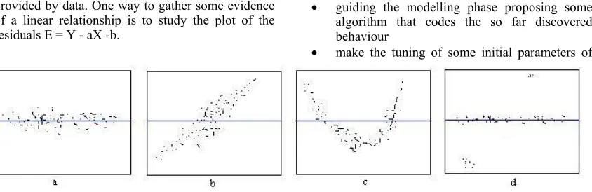
provided by data. One way to gather some evidence of a linear relationship is to study the plot of the residuals E = Y - aX -b.

In fact, if the assumption of a linear relationship between variable X and Y holds, the distribution of the residuals should follow a normal distribution with mean 0 (see figure 1(a)).

If the residuals follows a linear trend different from the horizontal line then the parameters of the estimation are wrong but the linear relationship assumption still holds (see figure 1(b)).

If the residuals follow a trend that is not linear then the assumption of linear dependency of Y from Y does not hold anymore and the estimator model is at least quadratic (see figure 1(c)). In this case linear regression is not useful anymore and a polynomial regression technique should be used.

If the trend is linear but a limited number of values differ significantly from the others then these values are called 'outliers' (see figure 1(d)). In this case the data model is subject to some disturbances that could be explained by error in data gathering or by exceptions in the model. In data mining there are well founded techniques to study the residuals and to manage the outliers.

A first phase of model estimation and study of residuals is usually the first step when there is the need to catch the basic dependencies between continuous parameters of a system.

6.5 Multiple regression

In multiple regression, as well as in the analysis of variance, the goal is to find relationships between variables of a system. The difference in multiple regression, and in regression in general as we outlined in previous section, is that such method tries to estimate such relationship rebuilding an equation that describe the behaviour of one or more dependant variables in function of one or more independent variables. There is more than one method in order to operate such regression whose main distinction can be seen from linear methods (where the equation obtained is linear in the input parameters) and non-linear methods (where the equation can be a polynomial or other functions). Pushing further the concept of preliminary analysis of the system to simulate, we can use multiple regression in order to:

• guiding the modelling phase proposing some algorithm that codes the so far discovered behaviour

• make the tuning of some initial parameters of

the simulation before the simulation starts • use the multiple regression above the real

system and the modelled one in order to provide a degree of adherence of the model to the real world

6.6 Cluster analysis

In cluster analysis the goal is to retrieve some collections of individuals whose description (or behaviour) is alike. In clustering analysis, the users can define a distance measure based on the properties of single agents. Moreover he can recognises if, within the system, are present well-defined set of individuals that are similar, based on the given distance measure (for an overview of conceptual clustering see Kaufman and Rousseeuw, 1990).

This is useful in order to decrease the number of elements to describe within the system. In fact, instead of focusing over the single agent behaviour in an object-oriented way, the user could look at the system as a set of clusters whose elements are in some way equivalent. Recognizing the fact that the description of single elements can be summarized by the description of few clusters can help to decrease the heterogeneity of the system.

6.7 Association rules

values is allowed. For example, we can observe the fact that in 90% of the cases if variable a = 1 then b = 0. This is not a deterministic knowledge base but it can be useful to abstract the expected behaviour of a population, providing a degree of adherence of the model to the observed data. A well known mechanism for discovering such kind of fuzzy rules are the Bayesian networks that use the theorem of Bayes about the conditional probabilities in order to train a network of discrete variables. Before applying such methods we can transform continuous input variables into categorical variables sampling the input domain into a predefined set of intervals and using the belonging to an interval as a categorical data. This is a way to abstract the data (as w have seen in section 5.3) and the model in order to lower the level of details and to provide a higher informative description of the system. The causal semantics associated to the results and its algorithmic nature provide us with a natural instrument to explore the hidden model followed by the system

6.8 Iterative process in modelling phase

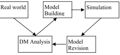
By using the above described methods, and many others not mentioned here, we can define a modelling and model revision process. Such process starts from the first task of model building (Model Building task in Figure 1) where a first proposal of model is done and will be tested after various runs. As we introduced in the first part of the paper, such task suffers from a set of initial hypothesis and it produces a first proposal of model used in the simulations. In this very first phase Data Mining (DM Analysis in Figure 1) can be used in order to make safe hypothesis over the real behaviour of the system (or at least for that portion of the behaviour that is observable, simulation is a good way to discover new scenarios that are not observed before).

Figure 2 : DM revision process applied to AB Simulation

When the simulation has produced a good amount of observations to work with (Simulation task in figure 1) a new phase of Data Mining analysis can be used to make hypothesis above the model produced (DM Analysis task in figure 1). Such results could validate or refuse the initial hypothesis about the real world and could guide a revision process in order to

refine our knowledge about the overall system (Model Revision task in figure 1).

Such iterative process could produce finer and finer model hypothesis until a desired convergence is found. Moreover, during the revision process the user could have a sound statistical theory as a guidance that provides him/her with a measure of the fitness of the model.

7. MULTIRUN AND PARAMETERS TUNING

Many agent based models, for their construction, are very "parameter sensitive", in the sense that a different combination of initial values or even a negligible variation of some of them can lead to very different results in the long run. This is realistic, since most of the systems studied with this methodology are complex and chaotic, but can lead to inappropriate results if the starting parameters are not finely chosen.

Besides, this is also a problem for validation; if the results are very dependant from the parameters, but not necessarily in a linear way, it becomes very difficult to analytically find statistical synthetic results that could describe the phenomenon.

For this reason we propose a brute-force method to explore the parameters space and thus allowing a data-mining analysis on the obtained results, linked with the parameters used. We call this approach “Parameters Tuning by repeated execution” (Remondino, 2005) and it allows an exhaustive exploration in order to find patterns and hidden dependencies.

This is performed by modifying one parameter at a time, by leaving the others unchanged (ceteris paribus) and then running the simulation for an equal number of steps and examine the output.

This is done mainly for two reasons:

• find hidden dependencies and patterns among parameters and results;

• being able to determine which are the “best'' parameters to get realistic results, in order to empirically validate the simulation according to an existing situation and to perform what-if analysis and simulate situations different from the real ones.

Determining the parameters stepping interval is very important task; in particular, for discrete values, it’s enough to consider the tinier possible step (e.g. if the parameter is “agents number”, then we can change it of 1 at a time, and so on). For continuous values it’s much more difficult to select the right stepping interval, to be selected properly for each individual case, according to the vision of the model and its detail.

Model Building

Real world Simulation

7.1 Application to an Agent Based Model of a Biological Phenomenon

In this paragraph it will be shown how multirun techniques can be effective in discovering patterns from aggregate data. An example is shown based on a model described in Remondino (2005) and Remondino and Cappellini (2005), inspired to a biological phenomenon involving some species of cicadas.

Magicicada is the genus of the 13 and 17 year periodical cicadas of eastern North America; these insects display a unique combination of long life cycles, periodicity, and mass emergences. Their nymphs live underground and stay immobile before constructing an exit tunnel in the spring of their 13th or 17th year, depending on the species. Once out, the adult insects live only for a few weeks with one sole purpose: reproduction. Both 13 and 17 are prime numbers; why did the cicadas “choose” these lengths for their life cycles? One interesting hypothesis is that the prime number cycles were selected because they were least likely to emerge with other cycles. If that’s the case, then these lengths would have been selected via a sort of “tacit communication” by evolution. In this example we have an agent based model, depicting a world in which cicadas with different life cycles go outside and cross among them, creating other insects with a life cycle inherited from the parents. In the simulation food is limited and predators exist, that can be satiated if the number of cicadas going out is large enough. The model could give us an empirical answer to the following question: is the “predator satiation” hypothesis enough, along with the limited food quantity, to explain the prime numbers based life cycle of these insects? But, above all, we can try to find if the model under these hypotheses can be a sort of biological prime numbers generator.

In the model, a slightly different reproduction rate, or a negligible variation of the cicadas/predators ratio can lead to very different results in the long run This is why the multirun methodology can give aggregate results by considering all the possible combinations of parameters. Basically a MultiRun is a “super Model” class that launches sub-models, by changing a single parameter at each run, while the others remain the same.

In the model we have some parameters that remain stationary (like the number of cicadas and the number of species, which differ only for the living period, which ranges from 1 to 20) and others that change in turn: the reproduction rate iterates from 0.1 to 10.1 with steps equal to 0.1, the probability to survive at birth ranges from 0.05 to 1.05 (step = 0.5) and the number of predators from 0 to 300 (step = 1).

In the “result space” explored with this discrete method, we found zones without any cicadas

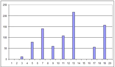
surviving, because of too many predators bundled with a low reproduction rate, or few chances to survive at birth. We collected the simulation results of every run after 20.000 years of evolution (tics), and represented them in figure 3, where the aggregate average result of 1220 total runs are shown. From these aggregate results we get a very interesting figure; by exploring the parameter space, we found that prime numbers are the most likely results to appear. In fact, the first five positions are indeed prime numbers (13, 19, 7, 11 and 5 respectively). We than have # 9, but after that we immediately find other two prime numbers, # 17 and # 3. With the exception of # 2 (which is probably too short a life cycle, to be selected), and of # 9 (about which, we don’t have an explanation) all the other numbers are prime and, in particular, all the prime numbers among 3 and 20 were discovered by the model. This result emerges only through the multirun analysis, since in separate runs we would have gotten much fuzzier figures; in this way we capture the most frequent occurrences when exhaustively exploring the parameters space.

Figure 3: Multirun aggregate normalized results

8. CONCLUSION

i.e.: by observing the real results coming from a real system and studying how well the model reproduces them, but also predictively, i.e.: by extrapolating a behaviour that could be used in “what if” analysis or to conduce experiments on those systems which don’t show a reproducible behaviour.

Last but not least, an original technique is introduced, called “Parameter Tuning by repeated execution”, which uses repeated execution of a model, to explore the parameters space, by discretely changing a parameter at a time, ceteris paribus. This can help finding hidden aggregate patterns when the model is highly parameter sensitive, by conducing comparative analysis on the collective results.

REFERENCES

Agrawal, R., Mannila, H., Srikant, R., Toivonen, H., and Verkamo, A. I. (1996). Fast discovery of association rules. In Fayyad, U. M., Piatetsky-Shapiro, G., Smyth, P., and Uthurusamy, R., eds., Advances in Knowledge Discovery and Data Mining. Menlo Park, CA: AAAI Press. Pp. 307-328

Bensaid N., & Mathieu P. (1997), A hybrid architecture for hierarchical agents

Bonabeau, E. 2002. “Agent-based modeling: Methods and techniques for simulating human systems”, PNAS 99 Suppl. 3: 7280-7287.

Brooks, R. A. (1990). Elephants Don't Play Chess, Designing Autonomous Agents, Pattie Maes, ed. Cambridge, MA: MIT Press

Fisher, R.A.. The goodness of fit of regression formulae, and the distribution of regression coefficients, J. Royal Statist. Soc., 85, pp. 597-612 (1922)

Forbus, K. (1984). Qualitative process theory. Artificial Intelligence,24, pp. 85-168

Franklin, S. (1995). Artificial Minds, Cambridge, MA: MIT Press

Franklin, S., & Graesser, A. (1997). Is it an Agent, or just a Program?: A Taxonomy for Autonomous Agents, Proceedings of the Agent Theories, Architectures, and Languages Workshop, Berlin (pp. 193-206). Springer Verlag.

Gilbert, N. and Terna, P. 2000. “How to build and use agent-based models in social science”, Mind & Society 1, 57-72

Ginsberg M. (1989). Universal planning: An (almost) universally bad idea. AI Magazine 10(4) pp. 40-44

Langton, C. (1989). Artificial Life, Redwood City, CA: Addison-Wesley

Kaufman, L. and Rousseeuw, P. J. Finding Groups in Data: an Introduction to Cluster Analysis. John Wiley & Sons, 1990.

Kim, D. (1993). "The link between individual and organizational learning", Sloan Management Review, Fall 1993, pp. 37-50

Mataric, M. (1995). Issues and approaches in the design of collective autonomous agents. Robotics and Autonomous Systems 16 (pp.321-331)

Ostrom T. (1988). Computer simulation: The third symbol system. Journal of Experimental Social Psychology, 24 (pp. 381-392)

Remondino, M. (2003). Agent Based Process Simulation and Metaphors Based Approach for Enterprise and Social Modeling, ABS 4 Proceedings (pp. 997). SCS Europ. Publish. House – ISBN 3-936-150-25-7

Remondino, M. (2005). Reactive and Deliberative Agents Applied to Simulation of Socio-Economical and Biological Systems, International Journal of Simulation (IJS3T), Volume 6, Number 12 & 13 – ISSN 1473-8031 (pp. 11- 25)

Remondino, M. and Cappellini A. (2005). Agent Based Simulation in Biology: the Case of Periodical Insects as Prime Numbers Generators, working paper

Salles, P and Bredeweg, B. (2003). Qualitative Reasoning about Population and Community Ecology. AI Magazine, 24(4), pp. 77-90

K. Takadama, T. Terano, and K. Shimohara: ``Design in Organizational Learning Agents'', The 1999 System information Symposium of SICE (The Society of Instrument and Control Engineers), pp. 139-144, 1999, (in Japanese).

Woolridge, M., & Jennings, N. (1995). Intelligent agents: Theory and practice. Knowledge Engineering Review 10(2) pp.115-152

BIOGRAPHY:

of the electric market and diffusion of technical innovations.