Logarithmic Asymptotics For Probability Of Component-Wise Ruin In A Two-Dimensional Brownian Model

Logarithmic Asymptotics for Probability

of Component-Wise Ruin in a Two-Dimensional

Brownian Model

Krzysztof De¸bicki1,†_{, Lanpeng Ji}2,_{* and Tomasz Rolski}1,†

1 _{Mathematical Institute, University of Wrocław, 50-137 Wrocław, Poland}

2 _{School of Mathematics, University of Leeds, Woodhouse Lane, Leeds LS2 9JT, UK}

* Correspondence: [email protected]

† These authors contributed equally to this work.

Received: 14 June 2019; Accepted: 29 July 2019; Published: 1 August 2019

Abstract: We consider a two-dimensional ruin problem where the surplus process of business lines is modelled by a two-dimensional correlated Brownian motion with drift. We study the ruin function P(u)for the component-wise ruin (that is both business lines are ruined in an infinite-time horizon), whereuis the same initial capital for each line. We measure the goodness of the business by analysing the adjustment coefficient, that is the limit of−lnP(u)/uasutends to infinity, which depends essentially on the correlationρof the two surplus processes. In order to work out the adjustment coefficient we solve

a two-layer optimization problem.

Keywords: adjustment coefficient; logarithmic asymptotics; quadratic programming problem; ruin probability; two-dimensional Brownian motion

1. Introduction

In classical risk theory, the surplus process of an insurance company is modelled by the compound Poisson risk model. For both applied and theoretical investigations, calculation of ruin probabilities for such model is of particular interest. In order to avoid technical calculations,diffusion approximationis often considered e.g., (Asmussen and Albrecher 2010;Grandell 1991;Iglehart 1969;Klugman et al. 2012), which results in tractable approximations for the interested finite-time or infinite-time ruin probabilities. The basic premise for the approximation is to let the number of claims grow in a unit time interval and to make the claim sizes smaller in such a way that the risk process converges to a Brownian motion with drift. Precisely, the Brownian motion risk process is defined by

R(t) =x+pt−σB(t), t≥0,

where x > 0 is the initial capital, p > 0 is the net profit rate and σB(t) models the net loss process

withσ > 0 the volatility coefficient. Roughly speaking, σB(t)is an approximation of the total claim

amount process by timetminus its expectation, the latter is usually called thepure premiumamount and calculated to cover the average payments of claims. The net profit, also calledsafety loading, is the component which protects the company from large deviations of claims from the average and also allows an accumulation of capital. Ruin related problems for Brownian models have been well studied; see, for example,Asmussen and Albrecher(2010);Gerber and Shiu(2004).

In recent years, multi-dimensional risk models have been introduced to model the surplus of multiple business lines of an insurance company or the suplus of collaborating companies (e.g., insurance and reinsurance). We refer toAsmussen and Albrecher(2010) [Chapter XIII 9] andAvram and Loke(2018); Avram and Minca(2017);Avram et al. (2008a,2008b);Albrecher et al.(2017);Azcue and Muler(2018); Azcue et al.(2019);Foss et al.(2017);Ji and Robert(2018) for relevant recent discussions. It is concluded in the literature that in comparison with the well-understood 1-dimensional risk models, study of multi-dimensional risk models is much more challenging. It was shown recently inDelsing et al.(2019) that multi-dimensional Brownian model can serve as approximation of a multi-dimensional classical risk model in a Markovian environment. Therefore, obtained results for multi-dimensional Brownian model can serve as approximations of the multi-dimensional classical risk models in a Markovian environment; ruin probability approximation has been used in the aforementioned paper. Actually, multi-dimensional Brownian models have drawn a lot of attention due to its tractability and practical relevancy.

Ad-dimensional Brownian model can be defined in a matrix form as R(t) =x+pt−X(t), t≥0, with X(t) =AB(t),

wherex = (x1,· · ·,xd)>,p = (p1,· · ·,pd)> ∈ (0,∞)dare, respectively, (column) vectors representing

the initial capital and net profit rate,A∈Rd×dis a non-singular matrix modelling dependence between

different business lines andB(t) = (B1(t), . . . ,Bd(t))>,t≥0 is a standardd-dimensional Brownian motion

(BM) with independent coordinates. Here>is the transpose sign. In what follows, vectors are understood as column vectors written in bold letters.

Different types of ruin can be considered in multi-dimensional models, which are relevant to the probability that the surplus of one or more of the business lines drops below zero in a certain time interval

[0,T]withTeither a finite constant or infinity. One of the commonly studied is the so-calledsimultaneous ruin probabilitydefined as

QT(x):=P

( ∃_t∈[0,T]

d

\

i=1

n

Ri(t)<0

o )

,

which is the probability that at a certain time t ∈ [0,T] all the surpluses become negative. Here for T < ∞, QT(x) is called finite-time simultaneous ruin probability, and Q∞(x) is called

infinite-time simultaneous ruin probability. Simultaneous ruin probability, which is essentially the hitting probability ofR(t)to the orthant{y∈Rd:yi <0,i=1, . . . ,d}, has been discussed for multi-dimensional

Brownian models in different contexts; see De¸bicki et al.(2018);Garbit and Raschel(2014). In Garbit and Raschel (2014), for fixed x the asymptotic behaviour of QT(x) as T → ∞ has been discussed.

Whereas, inDe¸bicki et al.(2018), the asymptotic behaviour, asu→∞, of the infinite-time ruin probability Q∞(x), with x = αu = (α1u,α2u, . . . ,α_du)>,αi > 0, 1 ≤ i ≤ d has been obtained. Note that it is

common in risk theory to derive the later type of asymptotic results for ruin probabilities; see, for example, Avram et al.(2008a);Embrechts et al.(1997);Mikosch(2008).

Another type of ruin probability is thecomponent-wise (or joint) ruin probabilitydefined as

PT(x):=P

( _d

\

i=1

n

∃_t∈[0,T]Ri(t)<0

o )

=P

( _d

\

i=1

n sup

ti∈[0,T]

(Xi(ti)−piti)>xi

o )

, (1)

which is the probability that all surpluses get below zero but possibly at different times. It is this possibility that makes the study ofPT(x)more difficult.

We refer toDelsing et al.(2019) for a comprehensive summary of related results. Due to the complexity of the problem, two-dimensional case has been the focus in the literature and for this case some explicit formulas can be obtained by using a PDE approach. Of particular relevance to the ruin probabilityPT(x)

is a result derived inHe et al.(1998) which shows that

P

( sup

t∈[0,T]

(X1(t)−p1t)≤x1, sup

s∈[0,T]

(X2(s)−p2s)≤x2

)

=ea1x1+a2x2+bT_f(x

1,x2,T),

wherea1,a2,bare known constants and f is a function defined in terms of infinite-series, double-integral

and Bessel function. Using the above formula one can derive an expression forPT(x)in two-dimensional

case as follows

PT(x) = 1−P

( sup

t∈[0,T]

(X1(t)−p1t)≤x1

) −P

( sup

s∈[0,T]

(X2(s)−p2s)≤x2

)

(2)

+P

( sup

t∈[0,T]

(X1(t)−p1t)≤x1, sup

s∈[0,T]

(X2(s)−p2s)≤x2

) ,

where the expression for the distribution of single supremum is also known; seeHe et al.(1998). Note that even though we have obtained explicit expression ofPT(x)in (2) for the two-dimensional case, it seems

difficult to derive the explicit form of the corresponding infinite-time ruin probabilityP_∞(x)by simply puttingT→∞in (2).

By assumingx = αu = (α1u,α2u, . . . ,α_du)>,αi > 0, 1≤ i ≤ d, we aim to analyse the asymptotic

behaviour of the infinite-time ruin probabilityP∞(x)asu→∞. Applying Theorem 1 inDe¸bicki et al.(2010) we arrive at the following logarithmic asymptotics

−1

ulnP∞(x) ∼ 1

2t>inf0v≥infα+pt

v>Σ−_t1v, asu→∞ (3)

provided Σt is non-singular, where pt := (p1t1,· · ·,pdtd)>, inequality of vectors are meant

component-wise, andΣ−_t 1is the inverse matrix of the covariance functionΣt of (X1(t1),· · ·,Xd(td)),

witht= (t1,· · ·,td)>and0= (0,· · ·, 0)>∈Rd. Let us recall that conventionally for two given positive

functionsf(·)andh(·), we write f(x)∼h(x)if limx→∞ f(x)/h(x) =1.

For more precise analysis onP_∞(x), it seems crucial to first solve the two-layer optimization problem in (3) and find the optimization pointst0. As it can be recognized in the following, when dealing with

d-dimensional case withd>2 the calculations become highly nontrivial and complicated. Therefore, in this contribution we only discuss a tractable two-dimensional model and aim for an explicit logarithmic asymptotics by solving the minimization problem in (3).

The rest of this paper is organised as follows. In Section2, we formulate the two-dimensional Brownian model and give the main results of this paper. The main lines of proof with auxiliary lemmas are displayed in Section3. In Section4we conclude the paper. All technical proofs of the lemmas in Section3 are presented in AppendixA.

2. Model Formulation and Main Results

Due to the fact that component-wise ruin probabilityP∞(x)does not change under scaling, we can simply assume that the volatility coefficient for all business lines is equal to 1. Furthermore, noting that the timelines for different business lines should be distinguished as shown in (1) and (3), we introduce a two-parameter extension of correlated two-dimensional BM defined as

(X1(t),X2(s)) =

B1(t), ρB1(s) +

q

1−ρ2B2(s)

, t,s≥0,

withρ∈(−1, 1)and mutually independent Brownian motionsB1,B2. We shall consider the following two

dependent insurance risk processes

Ri(t) =u+µit−Xi(t), t≥0, i=1, 2,

whereµ1,µ2 > 0 are net profit rates,uis the initial capital (which is assumed to be the same for both

business lines, as otherwise, the calculations become rather complicated). We shall assume without loss of generality thatµ1≤µ2. Here,µiis different frompi(see (1)) in the sense that it corresponds to the (scaled)

model with volatility coefficient standardized to be 1.

In this contribution, we shall focus on the logarithmic asymptotics of

P(u):=P∞(u(1, 1)>) = P{{∃t≥0R1(t)<0} ∩ {∃s≥0R2(s)<0}} (4)

= P

( sup

t≥0

(X1(t)−µ1t)>u, sup

s≥0

(X2(s)−µ2s)>u

)

, asu→∞.

Define

ˆ

ρ1=

µ1+µ2−p(µ1+µ2)2−4µ1(µ2−µ1)

4µ1

∈[0,1

2), ρ2ˆ =

µ1+µ2

2µ2

(5)

and let

t∗=t∗(ρ) =s∗=s∗(ρ):=

s

2(1−ρ)

µ2₁+µ2₂−2ρµ1µ2

. (6)

The following theorem constitutes the main result of this contribution.

Theorem 1. For the joint infinite-time ruin probability(4)we have, as u→∞,

−log(P(u))

u ∼

  

 

2(µ2+ (1−2ρ)µ1), if −1<ρ≤ρˆ1;

µ1+µ2+2/t∗

1+ρ , if ρˆ1<ρ<ρ2ˆ ;

2µ2, if ρˆ2≤ρ<1.

(b) One can easily check that adjustment coefficient as a function ofρis continuous, strictly decreasing on (−1, ˆρ2] and it is constant, equal to2µ2on[ρˆ2, 1). This means that as the two lines of business becomes more

positively correlated the risk of ruin becomes larger, which is consistent with the intuition. Define

g(t,s):= inf

x≥1+µ1t

y≥1+µ2s

(x,y)Σ−_ts1(x,y)>, t,s>0, (7)

whereΣ−_ts1is the inverse matrix of Σts = t ρt∧s

ρt∧s s

!

, witht∧s=min(t,s)and ρ∈(−1, 1).

The proof of Theorem1follows from (3) which implies that the logarithmic asymptotics forP(u)is of the form

−1

ulnP(u) ∼ g(t0)

2 , u→∞, (8)

where

g(t0) = inf

(t,s)∈(0,∞)2g(t,s), (9)

and Proposition3below, wherein we list dominating pointst0that optimize the functiongover(0,∞)2

and the corresponding optimal valuesg(t0).

In order to solve the two-layer minimization problem in (9) (see also (7)) we define fort,s>0 the following functions:

g1(t) = (1+µ1t) 2

t , g2(s) =

(1+µ2s)2

s ,

g3(t,s) = (1+µ1t, 1+µ2s)Σ−ts1(1+µ1t, 1+µ2s)>.

Sincet∧sappears in the above formula, we shall consider a partition of the quadrant(0,∞)2_{, namely} (0,∞)2=A∪L∪B, A={s<t}, L={s=t}, B={s>t}. (10) For convenience we denoteA={s≤t}= A∪LandB ={s≥t}=B∪L. Hereafter, all sets are defined on(0,∞)2_{, so(t,s)∈(0,∞)}2_{will be omitted.}

Note thatg3(t,s)can be represented in the following form:

g3(t,s) =

 



gA(t,s):= (1+µ2s)

2

s +

((1+µ1t)−ρ(1+µ2s))2

t−ρ2s , if(t,s)∈ A

gB(t,s):= (1+µ1t)

2

t +

((1+µ2s)−ρ(1+µ1t))2

s−ρ2t , if(t,s)∈ B.

(11)

Denote further

gL(s):=gA(s,s) =gB(s,s) = (1+

µ1s)2+ (1+µ2s)2−2ρ(1+µ1s)(1+µ2s)

(1−ρ2)s , s>0. (12)

In the next proposition we identify the so-called dominating points, that is, pointst0 for which

Notation: In the following, in order to keep the notation consistent,ρ ≤µ1/µ2is understood asρ < 1if µ1=µ2.

Proposition 3.

(i) Suppose that−1<ρ<0.

Forµ1<µ2we have

g(t0) =gA(tA,sA) =4(µ2+ (1−2ρ)µ1),

where,(tA,sA) = (tA(ρ),sA(ρ)):=

₁₋₂

ρ µ1 ,

1

µ2−2µ1ρ

is the unique minimizer of g(t,s),(t,s)∈(0,∞)2_.

Forµ1=µ2=:µwe have

g(t0) =gA(tA,sA) =gB(tB,sB) =8(1−ρ)µ,

where(tA,sA) =

₁₋₂

ρ

µ ,

1 (1−2ρ)µ

∈ A,(tB,sB):=

1 (1−2ρ)µ,

1−2ρ µ

∈ B are the only two minimizers of g(t,s),(t,s)∈(0,∞)2_.

(ii) Suppose that0≤ρ<ρˆ1. We have

g(t0) =gA(tA,sA) =4(µ2+ (1−2ρ)µ1),

where(tA,sA)∈ A is the unique minimizer of g(t,s),(t,s)∈(0,∞)2.

(iii) Suppose thatρ=ρˆ1. We have

g(t0) =gA(tA,sA) =4(µ2+ (1−2ρ)µ1),

where (tA,sA) = (tA(ρˆ1),sA(ρˆ1)) = (t∗(ρˆ1),s∗(ρˆ1)) ∈ L, is the unique minimizer of g(t,s),(t,s) ∈ (0,∞)2_{, with(t}∗_,s∗_{)defined in(6).}

(iv) Suppose thatρˆ1<ρ<ρˆ2. We have

g(t0) =gA(t∗,s∗) =gL(t∗) =

2

1+ρ(µ1+µ2+2/t ∗

),

where(t∗,s∗)∈ L is the unique minimizer of g(t,s),(t,s)∈(0,∞)2_.

(v) Suppose thatρ=ρ2ˆ . We have t∗(ρ2) =ˆ s∗(ρ2) =ˆ 1/µ2and

g(t0) =gA(1/µ2, 1/µ2) =gL(1/µ2) =g2(1/µ2) =4µ2,

where the minimum of g(t,s),(t,s)∈(0,∞)2_{is attained at(1/µ}

2, 1/µ2), with g3(1/µ2, 1/µ2) =g2(1/µ2)

and1/µ2is the unique minimizer of g2(s),s∈(0,∞).

(vi) Suppose thatρˆ2<ρ<1. We have

g(t0) =g2(1/µ2) =4µ2,

where the minimum of g(t,s),(t,s)∈(0,∞)2_{is attained when g(t,s) =g2(s).}

3. Proofs of Main Results

As discussed in the previous section, Proposition3combined with (8), straightforwardly implies the thesis of Theorem1. In what follows, we shall focus on the proof of Proposition3, for which we need to find the dominating pointst0by solving the two-layer minimization problem (9).

The solution of quadratic programming problem of the form (7) (inner minimization problem of (9)) has been well understood; for example,Hashorva (2005);Hashorva and Hüsler (2002) (see also Lemma 2.1 ofDe¸bicki et al.(2018)). For completeness and for reference, we present below Lemma 2.1 of De¸bicki et al.(2018) for the case whered=2.

We introduce some more notation. IfI⊂ {1, 2}, then for a vectora∈_R2_{we denote bya}

I= (ai,i∈I)

a sub-block vector ofa. Similarly, if furtherJ⊂ {1, 2}, for a matrixM= (mij)i,j∈{1,2}∈R2×2we denote by

MI J=MI,J= (mij)i∈I,j∈Jthe sub-block matrix ofMdetermined byIandJ. Further, writeMI I−1= (MI I)−1

for the inverse matrix ofMI Iwhenever it exists.

Lemma 5. Let M ∈ _R2×2 _{be a positive definite matrix. If b ∈}

R2\(−∞, 0]2, then the quadratic

programming problem

PM(b):Minimisex>M−1xunder the linear constraintx≥b

has a unique solutioneband there exists a unique non-empty index set I⊆ {1, 2}such that

e

bI=bI6=0I, M−_{I I}1bI>0I,

and if Ic={1, 2} \I6=∅, theneb_Ic =M_Ic_IM−_{I I}1b_I ≥b_Ic. Furthermore,

min

x≥bx

>_M−1_{x =}

e

b>M−1eb=b>_I M−_{I I}1b_I>0,

x>M−1eb = x>_I M−_{I I}1ebI =x>I M−I I1bI, ∀x∈R2.

For the solution of the quadratic programming problem (7) a suitable representation forg(t,s)is worked out in the following lemma.

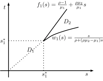
For 1> ρ > µ1/µ2, letD2 = {(t,s) :w1(s) ≤ t ≤ f1(s)}andD1 = (0,∞)2\D2, with boundary

functions given by

f1(s) = ρ−1

µ1

+ρµ2 µ1

s, w1(s) =

s

ρ+ (ρµ2−µ1)s, s≥0, (13)

and the unique intersection point off1(s),w1(s),s≥0, given by

s∗₁=s∗₁(ρ):= 1−ρ ρµ2−µ1

, (14)

D1

D2

s t

w1(s) = _ρ+(ρµs_2−µ1)s

f1(s) =ρ_µ−₁1+ρµ_µ12s

s∗1

s∗1

Figure 1.Partition of(0,∞)2_intoD 1,D2.

Lemma 6. Let g(t,s),t,s>0be given as in(7). We have: (i) If−1<ρ≤µ1/µ2,then

g(t,s) =g3(t,s), (t,s)∈(0,∞)2. (ii) If1>ρ>µ1/µ2,then

g(t,s) =

(

g3(t,s), if(t,s)∈D1

g2(s), if(t,s)∈D2.

Moreover, we have g3(f1(s),s) =g3(w1(s),s) =g2(s)for all s≥s1∗.

3.1. Proof of Proposition3

We shall discuss in order the case when−1<ρ<0 and the case when 0≤ρ<1 in the following

two subsections. In both scenarios we shall first derive the minimizers of the functiong(t,s)on regionsA andB(see (10)) separately and then look for a global minimizer by comparing the two minimum values. For clarity some scenarios are analysed in forms of lemmas.

3.1.1. Case−1<ρ<0

By Lemma6, we have that

g(t,s) =g3(t,s), (t,s)∈(0,∞)2.

We shall derive the minimizers ofg3(t,s)onA,Bseparately.

Minimizers ofg3(t,s)onA. We have, for any fixeds,

∂g3(t,s)

∂t =

∂gA(t,s)

∂t =0 ⇔ (µ1t+1−ρ−ρµ2s)(µ1t−(2µ1ρ

2_−ρµ2)s+

ρ−1) =0,

where the representation (11) is used. Two roots of the above equation are:

t1=t1(s):=

ρ−1+ρµ2s

µ1 ,

t2=t2(s):=

1−ρ+ (2µ1ρ2−ρµ2)s

µ1 . (15)

Note that, due to the form of the functiongA(t,s)given in (11), for any fixeds, there exists a unique

points. Next, we check if any ofti,i=1, 2, is larger thans. Sinceρ<0,t1<0<t2. So we check ift2>s.

It can be shown that

t2>s ⇔ (µ1+ρµ2−2µ1ρ2)s<1−ρ. (16)

Two scenariosµ1+ρµ2−2µ1ρ2≤0 andµ1+ρµ2−2µ1ρ2>0 will be distinguished.

Scenarioµ1+ρµ2−2µ1ρ2≤0. We have from (16) that

t1<0<s<t2,

and thus

inf

(t,s)∈A

g3(t,s) =inf

s>0fA(s),

where

fA(s):=gA(t2(s),s) =

(1+µ2s)2

s +4µ1((1−ρ) + (ρ

2

µ1−ρµ2)s).

Next, since

fA0(s) =0 ⇔ sA=sA(ρ):= _| 1

µ2−2ρµ1| =

1

µ2−2ρµ1 >0, (17)

the unique minimizer ofg3(t,s)onAis given by(tA,sA)with

tA :=t2(sA) =

1−2ρ µ1

.

Scenarioµ1+ρµ2−2µ1ρ2>0. We have from (16) that

t1<0<s<t2 ⇔ s< 1

−ρ

µ1+ρµ2−2µ1ρ2 =

1−ρ

ρ(µ2−µ1ρ) +µ1(1−ρ2) =:s

∗∗_{(ρ) =s}∗∗_{, (18)}

and in this case,

inf

(t,s)∈A

g3(t,s) =min

inf

0<s<s∗∗fA(s), inf_s≥s∗∗gL(s)

, (19)

wheregL(s)is given in (12). Note that

g0_L(s) =0 ⇔ s∗=s∗(ρ) =

s

2(1−ρ)

µ2₁+µ2₂−2ρµ1µ2

. (20)

Next, for−1<ρ<0 we have that (recalls∗∗given in (18))

s∗∗≥ 1−ρ

µ1(1−ρ2) >

1

µ1

≥ 1

µ2

>sA, s∗∗>

1−ρ µ1

Therefore, by (19) we conclude that the unique minimizer ofg3(t,s)onAis again given by(tA,sA).

Consequently, for all −1 < ρ < 0, we have that the unique minimizer of g3(t,s) on A is given by (tA,sA), and

inf

(t,s)∈Ag3(t,s) =gA(tA,sA) =4(µ2+ (1

−2ρ)µ1). (21)

Minimizers ofg3(t,s)onB. Similarly, we have, for any fixedt,

∂g3(t,s)

∂s =

∂gB(t,s)

∂s =0 ⇔ (µ2s+1−ρ−ρµ1t)(µ2s−(2µ2ρ

2_−ρµ1)t+

ρ−1) =0.

Two roots of the above equation are:

s1=s1(t):=

ρ−1+ρµ1t

µ2 ,

s2=s2(t):=

1−ρ+ (2µ2ρ2−ρµ1)t

µ2 . (22)

Next, we check if any ofsi,i=1, 2, is greater thant. Agains1<0<s2asρ<0. So we check ifs2>t.

It can be shown that

s2>t ⇔ (µ2+ρµ1−2µ2ρ2)t<1−ρ. (23)

Thus, for Scenarioµ2+ρµ1−2µ2ρ2≤0 we have that

s1<0<t<s2

and in this case

inf

(t,s)∈Bg3(t,s) =tinf>0fB(t),

with

fB(t):=gB(t,s2(t)) = (

1+µ1t)2

t +4µ2((1−ρ) + (ρ

2

µ2−ρµ1)t).

Next, note that

f_B0(t) =0 ⇔ tB=tB(ρ):=

1

|µ1−2ρµ2| =

1

µ1−2ρµ2 >0. (24)

Therefore, the unique minimizer ofg3(t,s)onBis given by(tB,sB)with

sB:=s2(tB) = 1

−2ρ

µ2 , (t,infs)∈Bg3(t,s) =gB(tB,sB) =4(µ1+ (1

−2ρ)µ2).

For Scenarioµ2+ρµ1−2µ2ρ2>0 we have from (23) that

s1<0<t<s2 ⇔ t<

1−ρ

µ2+ρµ1−2µ2ρ2 =

1−ρ

ρ(µ1−ρµ2) +µ2(1−ρ2) =:t ∗∗

In this case,

inf

(t,s)∈B

g3(t,s) =min

inf

0<t<t∗∗fB(t), inf_t≥t∗∗gL(t)

.

Though it is not easy to determine explicitly the optimizer, we can conclude that the minimizer should be taken at(tB,sB),(t∗,t∗)or(t∗∗,t∗∗), wheret∗=t∗(ρ) =s∗(ρ). Further, we have from the discussion in

(19) that

gA(tA,sA)<gL(s∗) =gL(t∗) =min(gL(t∗),gL(t∗∗)),

and

gB(tB,sB) =4(µ1+ (1−2ρ)µ2)≥4(µ2+ (1−2ρ)µ1) =gA(tA,sA).

Combining the above discussions onA,B, we conclude that Proposition3holds for−1<ρ<0.

3.1.2. Case 0≤ρ<1

We shall derive the minimizers ofg(t,s)onA,Bseparately. We start with discussions onB, for which we give the following lemma. Recallt∗(ρ) =s∗(ρ)defined in (20) (see also (6)),tB(ρ)defined in (24),t∗∗(ρ)

defined in (25) ands∗₁(ρ)defined in (14) forµ1/µ2<ρ<1. Note that where it applies, 1/0 is understood

as+∞and 1/∞is understood as 0.

Lemma 7. We have:

(a) The function t∗(ρ)is a decreasing function on[0, 1]and both tB(ρ)and s∗1(ρ)are decreasing functions on (µ1/µ2, 1).

(b) The function t∗∗(ρ)decreases from1/µ2atρ =0to some positive value and then increases to1/µ2atρ2ˆ

(defined in(5)) and then increases to+∞at the rootρˆ∈(0, 1]of the equationµ2+ρµ1−2µ2ρ2=0.

(c) For0≤ρ≤µ1/µ2, we have

tB(ρ)≥t∗∗(ρ), t∗(ρ)≥t∗∗(ρ),

where both equalities hold only whenρ=0andµ1=µ2.

(d) It holds that

t∗(ρˆ2) =tB(ρˆ2) =s∗₁(ρˆ2) =t∗∗(ρˆ2) = 1

µ2. (26)

Moreover, forµ1/µ2<ρ<1we have

(i) t∗(ρ)<s∗₁(ρ)for allρ∈(µ1/µ2, ˆρ2), t∗(ρ)>s∗₁(ρ)for allρ∈(ρˆ2, 1).

(ii) tB(ρ)<s∗1(ρ)for allρ∈(µ1/µ2, ˆρ2), tB(ρ)>s∗1(ρ)for allρ∈(ρˆ2, 1).

(iii) t∗∗(ρ)<s∗₁(ρ)for allρ∈(µ1/µ2, ˆρ2), t∗∗(ρ)>s∗₁(ρ)for allρ∈(ρ2ˆ , ˆρ).

(iv) t∗∗(ρ)<t∗(ρ)for allρ∈(µ1/µ2, ˆρ2), t∗∗(ρ)>t∗(ρ)for allρ∈(ρˆ2, ˆρ).

(v) t∗∗(ρ)<tB(ρ)for allρ∈(µ1/µ2, ˆρ2), t∗∗(ρ)>tB(ρ)for allρ∈(ρˆ2, ˆρ).

Recall that by definitiongL(s) =gA(s,s) =gB(s,s),s>0 (cf. (12)). For the minimum ofg(t,s)onB

Lemma 8. We have (i) If0≤ρ<ρˆ2, then

inf

(t,s)∈B

g(t,s) =gL(t∗) =

2

1+ρ(µ1+µ2+2/t ∗_),

where(t∗,t∗)is the unique minimizer of g(t,s)on B. (ii) Ifρ=ρˆ2, then t∗(ρˆ2) =s∗(ρˆ2) =1/µ2and

inf

(t,s)∈Bg(t,s) =gL(1/µ2) =g2(1/µ2) =4µ2,

where the minimum of g(t,s)on B is attained at(1/µ2, 1/µ2), with g3(1/µ2, 1/µ2) =g2(1/µ2)and1/µ2

is the unique minimizer of g2(s),s∈(0,∞). (iii) Ifρˆ2<ρ<1, then

inf

(t,s)∈Bg(t,s) =(t,sinf)∈D2

g2(s) =g2(1/µ2) =4µ2,

where the minimum of g(t,s)on B is attained when g(t,s) =g2(s)on D2(see Figure1).

Next we consider the minimum ofg(t,s)onA. Recalls∗(ρ)defined in (20),sA(ρ)defined in (17)

ands∗∗(ρ)defined in (18). We first give the following lemma. Lemma 9. We have

(a) Both s∗(ρ)and s∗∗(ρ)are decreasing functions on[0, 1]. (b) Thatρˆ1is the unique point on[0, 1)such that

sA(ρˆ1) =s∗∗(ρˆ1) =s∗(ρˆ1),

and

(i) sA(ρ)<s∗∗(ρ)for allρ∈[0, ˆρ1), sA(ρ)>s∗∗(ρ)for allρ∈(ρˆ1, 1),

(ii) s∗(ρ)<s∗∗(ρ)for allρ∈[0, ˆρ1), s∗(ρ)>s∗∗(ρ)for allρ∈(ρ1ˆ , 1).

(c) For allµ1/µ2<ρ<1, it holds that s∗∗(ρ)<s∗₁(ρ).

For the minimum ofg(t,s)onAwe have the following lemma. Lemma 10. We have

(i) If0≤ρ<ρˆ1, then

inf

(t,s)∈A

g(t,s) =gA(tA,sA) =4(µ2+ (1−2ρ)µ1),

where(tA,sA)∈ A is the unique minimizer of g(t,s)on A.

(ii) Ifρ=ρˆ1, then

inf

(t,s)∈A

g(t,s) =gA(tA,sA) =4(µ2+ (1−2ρ)µ1),

(iii) Ifρ1ˆ <ρ<ρ2ˆ , then

inf

(t,s)∈Ag(t,s) =gL(s

∗_{) =} 2

1+ρ(µ1+µ2+2/s ∗_),

where(s∗,s∗)is the unique minimizer of g(t,s)on A. (iv) Ifρ=ρˆ2, then t∗(ρˆ2) =s∗(ρˆ2) =1/µ2and

inf

(t,s)∈Ag(t,s) =gL(s

∗_{) =g2(1/}

µ2) =4µ2,

where the minimum of g(t,s)on A is attained at(1/µ2, 1/µ2), with g3(1/µ2, 1/µ2) =g2(1/µ2).

(v) Ifρˆ2<ρ<1, then

inf

(t,s)∈Ag(t,s) =g2(1/µ2) =4µ2,

where the minimum of g(t,s)on A is attained when g(t,s) =g2(s)on D2(see Figure1).

Consequently, combining the results in Lemma8and Lemma10, we conclude that Proposition3 holds for 0≤ρ<1. Thus, the proof is complete.

4. Conclusions and Discussions

In the multi-dimensional risk theory, the so-called “ruin” can be defined in different manner. Motivated by diffusion approximation approach, in this paper we modelled the risk process via a multi-dimensional BM with drift. We analyzed the component-wise infinite-time ruin probability for dimensiond=2 by solving a two-layer optimization problem, which by the use of Theorem 1 from De¸bicki et al.(2010) led to the logarithmic asymptotics forP(u) asu → ∞, given by explicit form of the adjustment coefficientγ = g(t0)/2 (see (8)). An important tool here is Lemma5on the quadratic

programming, cited fromHashorva(2005). In this way we were also able to identify the dominating points by careful analysis of different regimes forρand specify three regimes with different formulas for γ(see Theorem1). An open and difficult problem is the derivation of exact asymptotics forP(u)in (4),

for which the problem of finding dominating points would be the first step. A refined double-sum method as inDe¸bicki et al.(2018) might be suitable for this purpose. A detailed analysis of the case for dimensions d>2 seems to be technically very complicated, even for getting the logarithmic asymptotics. We also note that a more natural problem of consideringRi(t) =αiu+µit−Xi(t), with generalαi >0,i=1, 2, leads to

much more difficult technicalities with the analysis ofγ.

Define the ruin time of component i, 1 ≤ i ≤ d, by Ti = min{t : Ri(t) < 0} and let

T(1)≤T(2)≤. . .≤T(d) be the order statistics of ruin times. Then the component-wise infinite-time

ruin probability is equivalent to P

n

T₍d)<∞

o

while the ruin time of at least one business line is

Tmin = T(1) = miniTi. Other interesting problems like P

n

T_(j)<∞o have not yet been analysed. For instance, it would be interesting ford = 3 to study the case T(2). The general scheme on how

to obtain logarithmic asymptotics for such problems was discussed inDe¸bicki et al.(2010).

Random vectorX¯ = (sup_t≥0(X1(t)−p1t), . . . , supt≥0(Xd(t)−pdt))>has exponential marginals and

in this contribution, it would be interesting to find the correlation between sup_t≥0(X1(t)−µ1t)and

sup_t≥0(X2(t)−µ2t).

Author Contributions: Investigation, K.D., L.J., T.R.; writing–original draft preparation, L.J.; writing–review and editing, K.D., T.R.

Funding: T.R. & K.D. acknowledge partial support by NCN grant number 2015/17/B/ST1/01102 (2016-2019).

Acknowledgments:We are thankful to the referees for their carefully reading and constructive suggestions which significantly improved the manuscript.

Conflicts of Interest:The authors declare no conflict of interest. The funders had no role in the design of the study; in the collection, analyses, or interpretation of data; in the writing of the manuscript, or in the decision to publish the results.

Abbreviations

The following abbreviations are used in this manuscript:

BM Brownian motion

Appendix A

In this appendix, we present the proofs of the lemmas used in Section3.

Proof of Lemma6. Referring to Lemma5, we have, for any fixedt,s, there exists a unique index set I(t,s)⊆ {1, 2}

such that

g(t,s) = (1+µ1t, 1+µ2s)I(t,s)(Σts)−_I(t1_,s),I(t,s)(1+µ1t, 1+µ2s)>I(t,s), (A1)

and

(Σts)−_I(1_t,s),I(t,s)(1+µ1t, 1+µ2s)>_I(t,s)>0I(t,s). (A2)

SinceI(t,s) ={1},{2}or{1, 2}, we have that

(S1) On the setE1={(t,s):ρt∧s s−1(1+µ2s)≥(1+µ1t)}, g(t,s) =g2(s)

(S2) On the setE2={(t,s):ρt∧s t−1(1+µ1t)≥(1+µ2s)}, g(t,s) =g1(t)

(S3) On the setE3= (0,∞)2\(E1∪E2), g(t,s) =g3(t,s).

Clearly, ifρ≤0 then

E1=E2=∅, E3= (0,∞)2.

In this case,

g(t,s) =g3(t,s), (t,s)∈(0,∞)2_.

Next, we focus on the case whereρ>0. We consider the regionsAandBseparately.

Analysis onA. We have

A1=A∩E1={s≤t≤ f1(s)}, f1(s) = ρ−1

µ1

+ρµ2 µ1

s, A2=A∩E2={s≤t≤ f2(s)}, f2(s) =

ρs

A3=A∩E3={t≥s,t>max(f1(s),f2(s))}.

Next we analyse the intersection situation of the functions f(s) =s,f1(s),f2(s)on regionA.

Clearly, for anys>0 we have f2(s)<s. Furthermore, f1(s) = f2(s)has a unique positive solutions1

given by

s1= 1

−ρ ρ(µ2−ρµ1)

.

Finally, forρµ2≤µ1we have that f1(s)does not intersect with f(s)on(0,∞)but forρµ2>µ1the

unique intersection point is given bys₁∗>s1(cf. (14)). To conclude, we have, forρ≤µ1/µ2,

g(t,s) =g3(t,s), (t,s)∈ A, and forρ>µ1/µ2,

g(t,s) =

(

g3(t,s), if(t,s)∈A∩ {t≥max(s,f1(s)),t> f1(s)} g2(s), if(t,s)∈A∩ {s≤t≤ f1(s)}.

Additionally, we have from Lemma5g3(f1(s),s) =g2(s)for alls≥s∗₁.

Analysis onB. The two scenariosρ≤µ1/µ2andρ>µ1/µ2will be considered separately. Forρ≤ µ1/µ2, we have

B1=B∩E1={t<s≤h1(t)}, h1(t) =

ρt

1+ (µ1−ρµ2)t,

B2=B∩E2={t<s≤h2(t)}, h2(t) = ρ−1

µ2

+ρµ1 µ2

t, B3=B∩E3={s>max(t,h1(t),h2(t))}.

It is easy to check that

t>h1(t), t>h2(t), ∀t>0, and thus

g(t,s) =g3(t,s), (t,s)∈ B. Forρ>µ1/µ2, we have

B1=B∩E1={w1(s)≤t<s}, w1(s) = s

ρ+ (ρµ2−µ1)s,

B2=B∩E2={w2(s)≤t<s}, w2(s) = 1

−ρ µ1ρ +

µ2

µ1ρs,

B3=B∩E3={t<min(s,w1(s),w2(s))}.

Next we analyze the intersection situation of the functionsw(s) =s,w1(s),w2(s)on regionB. Clearly, for anys > 0,w2(s) > s. w1(s)andw2(s)do not intersect on(0,∞). w(s)andw1(s)has a unique intersection points∗₁(cf. (14)).

To conclude, we have, forρ≤µ1/µ2,

and forρ>µ1/µ2,

g(t,s) =

(

g3(t,s), if(t,s)∈B∩ {t<min(s,w1(s))} g2(s), if(t,s)∈B∩ {w₁(s)≤t<s}. Additionally, it follows from Lemma5thatg3(w1(s),s) =g2(s)for alls≥s∗₁.

Consequently, the claim follows by a combination of the above results. This completes the proof.

Proof of Lemma7. (a) The claim fort∗(ρ)follows by noting its following representation:

t∗(ρ) =s∗(ρ) =

s

2(1−ρ)

µ2₁+µ2₂−2µ1µ2+2µ1µ2−2ρµ1µ2 =

v u u t

2

(µ1−µ2)2

1−ρ +2µ1µ2

.

The claims fortB(ρ)ands₁∗(ρ)follow directly from their definition.

(b) First note that

t∗∗(0) =t∗∗(ρ2) =ˆ 1

µ2

.

Next it is calculated that

∂t∗∗(ρ)

∂ρ =

−2µ2ρ2+4µ2ρ−µ1−µ2 (µ2+ρµ1−2µ2ρ2)2 .

Thus, the claim of (b) follows by analysing the sign of ∂t∗∗(ρ)

∂ρ over(0, ˆρ).

(c) For any 0≤ρ≤µ1/µ2we have|µ1−2ρµ2| ≤µ1and thus

tB(ρ)≥ 1

u1

≥ 1 u2

≥ 1−ρ u2(1−ρ2) ≥

1−ρ

ρ(µ1−ρµ2) +µ2(1−ρ2) =t ∗∗_(ρ).

Further, since

µ2₁+µ2₂−2ρµ1µ2=µ1(µ1−ρµ2) +µ2(µ2−ρµ1)≤µ2(µ1−ρµ2) +µ2(µ2−ρµ1)≤2µ2₂(1−ρ),

it follows that

t∗(ρ)≥ 1

µ2

≥t∗∗(ρ).

(d) It is easy to check that (26) holds. For (i) we have

t∗(ρ)−s∗1(ρ) = (1−ρ)

1 f1(ρ)−

1 f2(ρ)

,

where

f1(ρ) =

s

(1−ρ)(µ2

1+µ22−2ρµ1µ2)

2 =

s

µ1µ2ρ2− (µ1+µ2) 2

2 ρ+

µ2₁+µ2₂

Analysing the properties of the above two functions, we havef1(ρ)is strictly decreasing on[0, 1]with

f1(0) =

s

µ2₁+µ2₂

2 >−µ1= f2(0), f1(1) =0≤µ2−µ1= f2(1),

and thus there is a unique intersection point of the two curves t∗(ρ) and s∗₁(ρ) which is ρ = ρ2ˆ .

Therefore, the claim of (i) follows. Similarly, the claim of (ii) follows since

tB(ρ)−s∗1(ρ) =

−(µ1+µ2)ρ+2µ2ρ2 (ρµ2−µ1)(2ρµ2−µ1).

Finally, the claims of (iii), (iv) and (v) follow easily from (a), (b) and (26). This completes the proof.

Proof of Lemma8. Consider first the case where 0≤ρ≤µ1/µ2. Recall (22). We check if any ofsi,i=1, 2,

is greater thant. Clearly,s1≤t. Next, we check whethers2>t. It is easy to check that

s2>t ⇔ t<t∗∗,

where (recall (25))

t∗∗=t∗∗(ρ) = 1−ρ

ρ(µ1−µ2ρ) +µ2(1−ρ2) >0.

Then

inf

(t,s)∈Bg3(t,s) =min

inf

0<t<t∗∗gB(t,s2(t)), inf_t≥t∗∗gB(t,t)

.

Consequently, it follows from (c) of Lemma7the claim of (i) holds for 0≤ρ≤µ1/µ2.

Next, we considerµ1/µ2 < ρ < 1. Recall the functionw1(s)defined in (13). Denote the inverse

function ofw1(s)by

ˆ

w1(t) = ρt

1−(ρµ2−µ1)t, t≥s ∗ 1.

We have from Lemma6that

gB(t, ˆw1(t)) =g2(t), t≥s1∗.

Further note that 1/µ2is the unique minimizer ofg2(s),s>0. Forµ1/µ2<ρ<ρˆ2, we have from (d)

in Lemma7that

inf

s∗₁≤sg2(s) =g2(s

∗

1) =gL(s∗1)>gL(t∗),

and further

inf

(t,s)∈Bg(t,s) = min(0<inft<t∗∗gB(t,s2(t)),t∗∗inf_≤t<s∗

1

gB(t,t), inf

s₁∗≤tgB(t, ˆw1(t)), infs∗₁≤sg2(s))

= gB(t∗,t∗) =gL(t∗),

Forρ=ρ2ˆ , because of (26) we have

inf

(t,s)∈Bg(t,s) = min(0<tinf<1/µ2

gB(t,s2(t)), inf

1/µ2≤t

gB(t, ˆw1(t)), inf 1/µ2≤s

g2(s)) = gB(1/µ2, 1/µ2) =gL(1/µ2) =g2(1/µ2),

and the unique minimum ofg(t,s)onBis attained at(1/µ2, 1/µ2). Moreover, for all ˆρ2<ρ<1 we have

s2(tB) =wˆ1(tB) =

1

µ2 >s∗₁.

Thus,

inf

(t,s)∈Bg(t,s) = min(0<inft<tB

gB(t,s2(t)), inf tB≤t

gB(t, ˆw1(t)), inf s∗

1≤s

g2(s)) = gB(tB, 1/µ2) =g2(1/µ2),

and the unique minimum of g(t,s)on Bis attained when g(t,s) = g2(s) onD2. This completes the

proof.

Proof of Lemma9. (a) The claim fors∗(ρ)has been shown in the proof of (a) in Lemma7. Next, we show the claim fors∗∗(ρ), for which it is sufficient to show that ∂s∗∗_∂ρ(ρ) <0 for allρ∈[0, 1]. In fact, we have

∂s∗∗(ρ)

∂ρ =

−2µ1ρ2+4µ1ρ−µ1−µ2 (µ1+ρµ2−2µ1ρ2)2 <0.

(b) In order to prove (i), the following two scenarios will be discussed separately:

(S1). µ2<2µ1; (S2). µ2≥2µ1.

First consider (S1). If 0≤ρ< ₂µ_µ2 1, then

sA(ρ)−s∗∗(ρ) = (µ1+

ρµ2−2µ1ρ2)−(1−ρ)(µ2−2ρµ1) (µ2−2ρµ1)(µ1+ρµ2−2µ1ρ2)

= f(ρ)

(µ2−2ρµ1)(µ1+ρµ2−2µ1ρ2),

where

f(ρ) =−4µ1ρ2+2(µ2+µ1)ρ−µ2+µ1.

Analysing the functionf, we conclude that

f(ρ)<0, for ρ∈[0, ˆρ1), f(ρ)>0, for ρ∈(ρ1ˆ , µ2

2µ1 ).

Further, for µ2

2µ1 ≤ρ<1 we have

sA(ρ)−s∗∗(ρ) =

µ1+µ2−2µ1ρ

Thus, the claim in (i) is established for (S1). Similarly, the claim in (i) is valid for (S2) . Next, note that

s∗(ρ)−s∗∗(ρ) = (1−ρ)

1 f1(ρ)−

1 f2(ρ)

with

f1(ρ) =

s

(1−ρ)(µ2

1+µ22−2ρµ1µ2)

2 =

s

µ1µ2ρ2−(µ1+µ2) 2

2 ρ+

µ2₁+µ2₂

2 f2(ρ) = µ1+ρµ2−2µ1ρ2.

Analysing the properties of the above two functions, we havef1(ρ)is strictly decreasing on[0, 1]with

f1(0) =

s

µ2₁+µ2₂

2 ≥µ1= f2(0), f1(1) =0≤µ2−µ1= f2(1),

and thus there is a unique intersection pointρ∈(0, 1)ofs∗(ρ)ands∗∗(ρ). It seems not clear at the moment

whether this unique point is ˆρ1or not, since we have to solve a polynomial equation of order 4. Instead, it is

sufficient to show that

sA(ρˆ1) =s∗(ρˆ1). (A3)

In fact, basic calculations show that the above is equivalent to

(2µ1ρˆ1−(u1+µ2))f(ρˆ1) =0

which is valid due to the fact that f(ρˆ1) =0. Finally, the claim in (c) follows since

ρµ2−µ1<µ1+ρµ2−2ρ2µ1.

This completes the proof.

Proof of Lemma10. Two cases ˆρ1≤µ1/µ2and ˆρ1>µ1/µ2should be distinguished. Since the proofs for

these two cases are similar, we give below only the proof for the more complicated case ˆρ1≤µ1/µ2.

Note that, for 0≤ρ≤µ1/µ2, as in (19),

inf

(t,s)∈Ag(t,s) =(t,infs)∈Ag3(t,s) =min

inf

0<s<s∗∗fA(s), inf_s≥s∗∗gL(s)

,

and thus the claim for 0≤ρ≤µ1/µ2follows directly from (i)–(ii) of (b) in Lemma9.

Next, we consider the caseµ1/µ2 < ρ < ρˆ2(note here ˆρ1 < µ1/µ2 < ρ). We have by (i) of (d) in

Lemma7and (i)–(ii) of (b) in Lemma9that

s∗∗(ρ)<s∗(ρ) =t∗(ρ)<s∗₁(ρ), s∗₁(ρ)> 1 µ2

Thus, it follows from Lemma6that

inf

(t,s)∈Ag(t,s) = min 0<infs<s∗∗gA(t2(s),s),_s∗∗inf_≤s≤s∗

1

gA(s,s), inf s∗

1<s

gA(f1(s),s), inf s∗

1<s

g2(s)

!

= gA(t∗,s∗) =gL(s∗),

and(t∗,s∗)∈Lis the unique minimizer ofg(t,s)onA. Here we used the fact that inf

s₁∗<sgA(f1(s),s) =sinf₁∗<sg2(s) =gA(f1(s

∗

1),s∗1) =g2(s∗1)>gL(s∗).

Next, ifρ=ρˆ2, then

s∗₁(ρˆ2) =s∗(ρˆ2) = 1 µ2

,

and thus

inf

(t,s)∈A

g(t,s) = min

inf

0<s<s∗∗gA(t2(s),s),_s∗∗_≤inf_s≤1/µ

2

gA(s,s), inf

1/µ2<s

gA(f1(s),s), inf 1/µ2<s

g2(s)

= gA(1/µ2, 1/µ2) =gL(1/µ2) =g2(1/µ2).

Furthermore, the unique minimum of g(t,s) on A is attained at (1/µ2, 1/µ2),

withg3(1/µ2, 1/µ2) =g2(1/µ2).

Finally, for ˆρ2<ρ<1, we have

s∗∗(ρ)<s∗₁(ρ)<s∗(ρ)< 1 µ2

, sA(ρ)>s∗∗(ρ),

and thus

inf

(t,s)∈Ag(t,s) = min 0<infs<s∗∗gA(t2(s),s),s∗∗inf_≤s≤s∗

1

gA(s,s), inf

s∗₁<sgA(f1(s),s), infs∗₁<sg2(s)

!

= g2(1/µ2),

where the unique minimum of g(t,s)on Ais attained when g3(t,s) = g2(s)on D2. This completes

the proof.

References

Albrecher, Hansjörg, Pablo Azcue, and Nora Muler. 2017. Optimal dividend strategies for two collaborating insurance companies. Advances in Applied Probability49: 515–48. [CrossRef]

Asmussen, Søren, and Hansjörg Albrecher. 2010. Ruin Probabilities, 2nd ed. Advanced Series on Statistical Science & Applied Probability, 14. Hackensack: World Scientific Publishing Co. Pte. Ltd.

Avram, Florin, and Sooie-Hoe Loke. 2018. On central branch/reinsurance risk networks: Exact results and heuristics.

Risks6: 35. [CrossRef]

Avram, Florin, and Andreea Minca. 2017. On the central management of risk networks. Advances in Applied Probability

49: 221–37. [CrossRef]

Avram, Florin, Zbigniew Palmowski, and Martijn R. Pistorius. 2008b. A two-dimensional ruin problem on the positive quadrant. Insurance: Mathematics and Economics42: 227–34. [CrossRef]

Azcue, Pablo, and Nora Muler. 2018. A multidimensional problem of optimal dividends with irreversible switching: A convergent numerical scheme.arXiv. arXiv:1804.02547.

Azcue, Pablo, Nora Muler, and Zbigniew Palmowski. 2019. Optimal dividend payments for a two-dimensional insurance risk process.European Actuarial Journal 9: 241–72. [CrossRef]

De¸bicki, Krzysztof, Enkelejd Hashorva, Lanpeng Ji, and Tomasz Rolski. 2018. Extremal behavior of hitting a cone by correlated Brownian motion with drift. Stochastic Processes and their Applications12: 4171–206. [CrossRef] De¸bicki, Krzysztof, Kamil MarcinKosi ´nski, Michel Mandjes, and Tomasz Rolski. 2010. Extremes of multidimensional

Gaussian processes. Stochastic Processes and their Applications120: 2289–301. [CrossRef]

Delsing, Guusje, Michel Mandjes, Peter Spreij, and Erik Winands. 2018. Asymptotics and approximations of ruin probabilities for multivariate risk processes in a Markovian environment.arXiv.arXiv:1812.09069.

Embrechts, Paul, Claudia Klüppelberg, and Thomas Mikosch. 1997. Modelling Extremal Events of Applications of Mathematics (New York). Berlin: Springer, vol. 33.

Foss, Sergey, Dmitry Korshunov, Zbigniew Palmowski, and Tomasz Rolski. 2017. Two-dimensional ruin probability for subexponential claim size. Probability and Mathematical Statistics2: 319–35.

Garbit, Rodolphe, and Kilian Raschel. 2014. On the exit time from a cone for Brownian motion with drift.

Electronic Journal of Probability19: 1–27. [CrossRef]

Gerber, Hans U., and Elias SW Shiu. 2004. Optimal Dvidends: Analysis with Brownian Motion. North American Actuarial Journal8: 1–20. [CrossRef]

Grandell, Jan. 1991. Aspects of Risk Theory. New York: Springer.

Hashorva, Enkelejd. 2005. Asymptotics and bounds for multivariate Gaussian tails. Journal of Theoretical Probability

18: 79–97. [CrossRef]

Hashorva, Enkelejd, and Jürg Hüsler. 2002. On asymptotics of multivariate integrals with applications to records.

Stochastic Models18: 41–69. [CrossRef]

He, Hua, William P. Keirstead, and Joachim Rebholz. 1998. Double lookbacks. Mathematical Finance8: 201–28. [CrossRef]

Iglehart, L. Donald. 1969. Diffusion approximations in collective risk theory. Journal of Applied Probability6: 285–92. [CrossRef]

Ji, Lanpeng, and Stephan Robert. 2018. Ruin problem of a two-dimensional fractional Brownian motion risk process.

Stochastic Models34: 73–97. [CrossRef]

Klugman, Stuart A., Harry H. Panjer, and Gordon E. Willmot. 2012. Loss Models: From Data to Decisions. Hoboken: John Wiley and Sons.

Kou, Steven, and Haowen Zhong. 2016. First-passage times of two-dimensional Brownian motion. Advances in Applied Probability48: 1045–60. [CrossRef]

Li, Junhai, Zaiming Liu, and Qihe Tang. 2007. On the ruin probabilities of a bidimensional perturbed risk model.

Insurance: Mathematics and Economics41: 185–95. [CrossRef]

Mikosch, Thomas. 2008. Non-life Insurance Mathematics. An Introduction with Stochastic Processes. Berlin: Springer. Rolski, Tomasz, Hanspeter Schmidli, Volker Schmidt, and Jozef Teugels. 2009. Stochastic Processes for Insurance and

Finance. Hoboken: John Wiley & Sons, vol. 505.

c