Random walk with barycentric self-interaction

Random walk with barycentric self-interaction

Francis Comets

Mikhail V. Menshikov

Stanislav Volkov

Andrew R. Wade

30th April 2011

Abstract

We study the asymptotic behaviour of a d-dimensional self-interacting random walk (Xn)n∈N(N:={1,2,3, . . .}) which is repelled or attracted by the centre of mass Gn = n−1Pn_i=1Xi of its previous trajectory. The walk’s trajectory (X1, . . . , Xn)

models a random polymer chain in either poor or good solvent. In addition to some natural regularity conditions, we assume that the walk has one-step mean drift

E_{[Xn+1−Xn|Xn−Gn=}x_]≈ρkx_k−βx_ˆ

forρ ∈ R _{and β ≥0. When β < 1 andρ >0, we show that Xn is transient with}

a limiting (random) direction and satisfies a super-diffusive law of large numbers: n−1/(1+β)Xnconverges almost surely to some random vector. Whenβ ∈(0,1) there

is sub-ballistic rate of escape. When β ≥0 and ρ ∈R _{we give almost-sure bounds}

on the norms kXnk, which in the context of the polymer model reveal extended and collapsed phases.

Analysis of the random walk, and in particular of Xn−Gn, leads to the study

of real-valued time-inhomogeneous non-Markov processes (Zn)n∈N on [0,∞) with

mean drifts of the form

E_{[Zn+1−Zn|Zn=x]≈ρx}−β₋x

n, (0.1)

whereβ ≥0 andρ∈R_{. The study of such processes is a time-dependent variation}

on a classical problem of Lamperti; moreover, they arise naturally in the context of the distance of simple random walk onZd_{from its centre of mass, for which we also}

give an apparently new result. We give a recurrence classification and asymptotic theory for processes Zn satisfying (0.1), which enables us to deduce the complete

recurrence classification (for anyβ ≥0) of Xn−Gnfor our self-interacting walk.

Keywords: Self-interacting random walk; self-avoiding walk; random walk avoiding its convex hull; random polymer; centre of mass; simple random walk; random walk average; limiting direction; law of large numbers.

AMS 2010 Subject Classifications: 60J05 (Primary) 60K40; 60F15; 82C26 (Secondary)

∗_{Universit´e Paris 7 (Diderot), Case courrier 7012, 2 Place Jussieu, 75251 Paris Cedex 05, France.} E-mail: [email protected].

†_{Department of Mathematical Sciences, University of Durham, South Road, Durham DH1 3LE, UK.} E-mail: [email protected].

‡_{Department of Mathematics, University of Bristol, University Walk, Bristol BS8 1TW, UK. E-mail:}

[email protected].

§_{Department of Mathematics and Statistics, University of Strathclyde, 26 Richmond Street, Glasgow} G1 1XH, UK. E-mail: [email protected].

1

Introduction

We study a self-interacting random walk. Self-interacting random processes, in which the stochastic behaviour depends on the entire previous history of the process, present many challenges for mathematical analysis (see e.g. [4,34] and references therein) and are often motivated by real applications.

Although not a random process in the same sense, theself-avoiding walkis a prototy-pical example of a self-interacting random walk that gives rise to important and difficult problems. Random self-avoiding walks were introduced to model the configuration of polymer molecules in solution. The sites visited by the walk represent the locations of the polymer’s constituent monomers; successive monomers are viewed as connected by chemical bonds. The classical self-avoiding walk (SAW) model takes uniform measure on

n-step self-avoiding paths inZd_{. In the important cases ofd∈ {2,3}, there are still major}

open problems for such walks: see for example [26,28] and [17, Chapter 7], or [37, Chapter 7] for a mathematical physics perspective.

Theloop-erased random walk(LERW), obtained by erasing chronologically the loops of a random walk, was introduced in [24] to study SAW, but it was soon realized that the two processes belong to different universality classes. For its independent interest, including applications to combinatorics and quantum field physics, LERW has received considerable attention and now there is a more precise picture of its behaviour, which shows fine dependence on the spatial dimension. In the planar case, the mean number of steps for LERW stopped at distance n is of order n5/4 _{[20], and the scaling limit is conformally}

invariant, described by the radial Schramm–Loewner evolution with parameter 2 [25]. A different perspective on polymer models concerns directed polymers, where the self-interaction is reduced to a trivial form but interesting phenomena arise from the interaction with the medium: see [14, 16] for recent surveys for localization on inter-faces (pinning, wetting) possibly with time-inhomogeneities (e.g. copolymers), and [9] for interactions with a time-space inhomogeneous medium leading to localization in the bulk. In the standard framework, SAW cannot be interpreted as a dynamic (or progressive) stochastic process. There have been many attempts to formulate genuine stochastic processes with similar behaviour to that of, or at least conjectured for, SAW. A recent model is the random walk onR2_{which at each step avoids the convex hull of its preceding}

values [2,39]. Unlike the conjectured behaviour of SAW, this model is ballistic (see [2,39]), i.e., it has a positive speed. The discrete version on Z2_{, the dynamic prudent walk, has}

been studied in [5]: it is ballistic with speed 3/7 (in the L1 _{norm), but, in contrast to}

the (conjecture for the) continuous model, it does not have a fixed direction (see [5]). Ballisticity is known for other types of self-interacting random walks: see [7, 18].

In this paper we consider a self-interacting random walk model that is a tractable alternative to SAW, and is distinguished from the models of [2,5,7,18,39] by exhibiting a range of possible scaling behaviour, including sub-ballisticity (i.e., zero speed) and super-diffusivity. Our model is tunable, with parameters that in principle can be estimated from real data, and it can be used to represent polymers in the extended phase (for good solvent) or collapsed phase (poor solvent). The self-interaction in the model at time n

Letd∈N_{:={1,2,3, . . .}. Our random walk will be a discrete-time stochastic process} X = (Xn)n∈N onRd. For n ∈N, set

Gn:=

1

n

n

X

i=1

Xi, (1.1)

the centre of mass (average) of {X1, . . . , Xn}. In addition to some regularity conditions

on X that we describe later, our main assumption will be that the one-step mean drift of the walk after n steps is of order kXn−Gnk−β in the direction ±(Xn−Gn), where

β ≥ 0 is a fixed parameter; here and subsequently k · k denotes the Euclidean norm on

Rd_{. Loosely speaking for the moment, we will suppose that for some ρ∈Rand β≥0,}

E_{[Xn+1−Xn |Xn−Gn =x]≈ρkxk}−β_{xˆ, (1.2)}

for anyn ∈N_andx∈Rd_{\{0}, where ˆx:=x/kxkdenotes a unit vector in thex-direction}

and 0 is the origin inRd_{. We attach no precise meaning to ‘≈’ in (1.2) (or elsewhere); it}

indicates that we are ignoring some terms and also that we have not yet formally defined all the terms present. We describe the model formally and in detail in Section 2 below.

The natural case of our model to compare to the walk that avoids its convex hull [2,39] has β = 0 and ρ > 0, when our walk has positive drift away from its current centre of mass. In ourβ = 0, ρ >0 setting we show that the walk has an asymptotic speed and an asymptotic direction, properties which are conjectured but not yet proved for the walk avoiding its convex hull [2, 39]. Our results however cover much more than this special case. For example, the case of our model that we might expect to be in some sense comparable to SAW ind= 2 has β= 1/3,ρ >0: see the discussion in Section 3.3 below. To give a flavour of our more general results, described in more detail in Section 2.2 below, we now informally describe our results in the case where (1.2) holds with

ρ > 0 and β ∈ [0,1). Under suitable regularity conditions, we show that X is transient, i.e. kXnk → ∞ a.s., and moreover we prove a strong law of large numbers that precisely

quantifies this transience: n−1/(1+β)_kX

nk is asymptotically constant, almost surely. In

addition, we show that Xn has a limiting direction, that is, Xn/kXnk converges a.s. to

some (random) unit vector. Thus we have, in this case, a rather complete picture of the asymptotic behaviour of Xn. For other regions of the (ρ, β) parameter space we have

other results, although we also leave some interesting open problems.

The self-interaction in the model is introduced via the presence of Gn in (1.2). If the

condition{Xn−Gn =x}in (1.2) is replaced by{Xn=x}then there is no self-interaction

in the drift, which instead points away from a fixed origin. Such non-homogeneous ‘centrally biased’ walks were studied by Lamperti in [21, Section 4] and [23, Section 5]; for more recent work see e.g. [13, 27, 31]. Considering the process of norms Zn = kXnk

leads to a process on [0,∞) with mean drift

E_{[Zn+1−Zn|Zn =x]≈ρ}′_x−β_{, (1.3)}

ignoring higher-order terms. Such ‘asymptotically zero-drift’ processes are of independent interest; the asymptotic analysis of such (not necessarily Markov) processes is sometimes known as Lamperti’s problem following pioneering work of Lamperti [21–23]. From the point of view of the recurrence classification of processes satisfying (1.3), the case β = 1 turns out to be critical, in which case the value of ρ′ _{∈ R is crucial: we give a brief}

We shall see below that considering the process Zn =kXn−Gnk with Xn satisfying

(1.2) leads to a more complicated form of (1.3). Loosely speaking, we will obtain

E_{[Zn+1−Zn|Zn =x]≈ρ}′_x−β ₋ x

n. (1.4)

We note that the two terms on the right-hand side of (1.4) are typically of the same order, as can be predicted by solving the corresponding differential equation, and so both contribute to the asymptotic behaviour.

Comparing (1.4) with (1.3), we see that the drift is now time- as well as space-dependent. (A different variation on (1.3) with this property was studied in [30], where processes with drift ρxα_n−β _{were considered.) Thus (1.4) is an interesting starting point}

for analysis in its own right. Additional motivation for (1.4) arises naturally from simple random walk (SRW) and its centre of mass: if Zn=kXn−Gnk whereXn is a symmetric

SRW on Zd _{and Gn its centre-of-mass as defined by (1.1), Zn satisfies (1.4) with β = 1}

and ρ′ _=ρ′_{(d); see Section 3.2 below.}

Let us step back from the general setting for a moment to state one consequence of our results, which is a (seemingly new) observation on SRW:

Theorem 1.1. Let d ∈ N_{. Suppose that (Xn)n∈N is a symmetric SRW on} Zd_{, and}

(Gn)n∈N is its centre-of-mass process as defined by (1.1). Then

(a) lim infn→∞kXn−Gnk<∞ a.s. for d∈ {1,2};

(b) limn→∞kXn−Gnk=∞ a.s. for d≥3.

P´olya’s recurrence theorem says that Xn is recurrent ind ≤2 and transient in d≥3,

while results of Grill [15] say that the centre-of-mass process Gn is recurrent only in

d= 1 and transient for d≥2. Thus the asymptotic behaviour of Xn−Gn is not trivial;

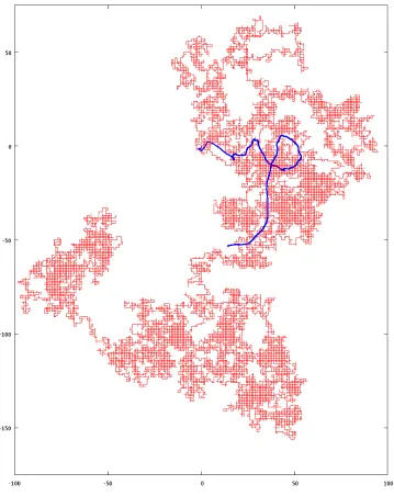
Theorem 1.1 says that it is recurrent if and only if d∈ {1,2}. In particular whend = 2,

Xn and Xn−Gn are both recurrent, but Gn is transient; see Figure 1 for a simulation.

Remark 1.1. Theorem 1.1 exhibits an amusing feature. With the notation∆n :=Xn+1−

Xn it is not hard to see from (1.1) that we may write (with X0 :=0)

Gn= n−1

X

i=0

1− i

n

∆i; Xn−Gn= n−1

X

i=0

i n

∆i.

It follows that (for fixedn)Xn−Gn andGn are very nearly time-reversalsof each other:

writing ∆′

i := ∆n−i we see that

Xn−Gn= n

X

i=1

1− i

n

∆′_i.

Despite this, the two processes behave very differently, as can be seen by contrasting Theorem 1.1 with Grill’s result [15].

It is natural to ask whether a continuous analogue of Theorem 1.1 holds. In the one-dimensional case, we would take Bt to be standard Brownian motion and Gt =

t−1Rt

0 Bsds, and ask about the joint behaviour of (Bt, Gt); in higher dimensions, writing

the d-dimensional Brownian motion as (Bt(1), . . . , B

(d)

t ), the ith component G

(i)

t−1Rt

0 B (i)

s ds, and different components are independent. We could not find a Brownian

analogue of Grill’s theorem [15] for (compact set) recurrence/transience of Gt explicitly

stated in the literature. The process (tGt)t≥0 is integrated Brownian motion, or the

Langevin process, see e.g. [3, 19] and references therein. The two-dimensional process (Bt, tGt)t≥0 is the Kolmogorov diffusion [19]. Theorem 1.1 gives basic information about

the joint behaviour of a discrete version of this process, under a re-scaling of the second coordinate.

Figure 1: Simulation of 4×104 _{steps of symmetric SRW starting at the origin ofZ}2 _and

its centre of mass process (thick line). [color online]

We finish this section with some comments on the relation of our model to the existing literature. We are not aware of any self-interacting random walk models similar to the one studied here (i.e., interacting with the previous history of the process, as summarized through the barycentre). In broad outline, our model is related to the vertex-reinforced random walk (see [34, Section 5.3]) in that the evolution of the walk depends on the sites previously visited. A significant difference is that in vertex-reinforced random walk this self-interaction is local, in that only the occupation of nearest-neighbours of the current site affects the law of the increment, whereas our interaction, mediated by the barycentre, is global. In the continuous setting, self-interacting diffusions (or ‘Brownian polymers’) with similar flavour and motivation to those of our model have also been studied over the last two decades or so, but are rather different in detail to the model considered here: see e.g. [4, 11, 32, 33] and references therein; some recent work on processes with self-attracting drift defined through a potential includes [6]. In the self-interacting diffusion setting, most of the results in the literature are concerned with the ergodic case; questions of recurrence/transience seem to have received little attention (particularly in dimensions greater than 1), and we do not know of any results on asymptotic directions. Also, it is typically assumed that the vector consisting of the process and its empirical average are Markovian, whereas our model is more general. See [32, Section 1] for a short survey.

2

The model and main results

2.1

Definitions and assumptions

We now define the stochastic process X := (Xn)n∈N on Rd (d ∈ N) that is our main

object of study. (We start at time n = 1 only so that (1.1) has the neatest form.) The process X will not be Markovian, as the distribution of Xn+1 will depend on the entire

history X1, . . . , Xn, although to a large extent this dependence will be mediated through

the current centre of mass Gn defined at (1.1). Formally, we suppose that (Xn)n∈N is

adapted to the filtration (Fn)n∈N; note that by (1.1) G1, . . . , Gn are Fn-measurable. We

use the notation P_{n[·] :=} P_{[· | Fn] and} E_{n[·] :=} E_{[· | Fn]. Throughout the paper we}

understand logx to mean logx if x≥1 and 0 otherwise.

We impose some specific assumptions on the law of ∆n :=Xn+1 −Xn given Fn. We

assume that for some B ∈(0,∞) and all n ∈N_,

P_{n[k∆nk ≤B] = 1, a.s.. (2.1)}

The assumption of uniformly bounded jumps can be replaced by an assumption on higher order moments at the expense of additional technical complications, but (2.1) is natural when the increments represent chemical bonds in a model for a polymer molecule.

Our next assumption will be a precise version of (1.2). We suppose that for some

ρ∈R _{and β ≥0, for anyn ∈}N_{, writing x=Xn−Gn for convenience,}

E_{n[∆n] =ρkxk}−β_xˆ+O(kxk−β_(logkxk)−2_{), a.s., (2.2)}

terms not involving n are understood to be uniform in n. To be clear, (2.2) is to be understood as, with Xn−Gn=x, as kxk → ∞,

sup

n∈N

ess supkE_{n[∆n]−ρkxk}−β_{xkˆ =O(kxk}−β_(logkxk)−2_).

We also need to assume a uniform ellipticity condition, to ensure that our random walk does not get ‘trapped’ in some subset of Rd_{. Let} S_{d :={e ∈}Rd _{: kek = 1} denote}

the unit-radius sphere in Rd_{. We suppose that there exists ε0 >0 such that}

ess inf

e∈S_d

P_{n[∆n·e≥ε0]≥ε0. (2.3)}

Write ∆n = (∆(1)n , . . . ,∆(nd)) in Cartesian components. An immediate consequence of

(2.3) is the following lower bound on second moments: a.s.,

min

i∈{1,...,d}

E_n[(∆(i)

n )2]≥2ε30 >0. (2.4)

Our primary standing assumption will be the following.

(A1) Let d∈ N_{. Let X := (Xn)n∈N be a stochastic process on}Rd _{and G := (G}

n)n∈N its

associated centre-of-mass process defined by (1.1). For definiteness, take X1 ∈ Rd

to be fixed. Suppose that for someB <∞,ε0 >0,ρ∈R, andβ ≥0 the conditions

(2.1), (2.2), and (2.3) hold.

In the examples discussed later (see Section 2.3), (Xn, Gn)n∈N will be a Markov

pro-cess, but we do not assume the Markov property in general.

When β = 1, as in the Lamperti case [21, 23] the value of ρ in (2.2) will turn out to be crucial. As in Lamperti’s problem, the recurrence classification depends on the relationship betweenρand the covariance structure of ∆n. To obtain an explicit criterion,

we impose additional regularity conditions on that covariance structure. Specifically, we sometimes suppose that (a) there exists σ2 _{∈(0,∞) such that, a.s.,}

E_n[(∆(i)

n )2] =σ2+o((logkXn−Gnk)−1), (i∈ {1, . . . , d}); (2.5)

and (b) for i, j distinct elements of {1, . . . , d}, a.s.,

E_n[∆(i)

n ∆(nj)] =o((logkXn−Gnk)−1). (2.6)

Thus for β ≥1, when necessary we will impose the following additional assumption.

(A2) The conditions (2.5) and (2.6) hold for some σ2 _∈(0,∞).

2.2

Results on self-interacting walk

Our first result, Theorem 2.1, constitutes the first part of our complete recurrence classifi-cation forXn−Gn. Since we are dealing with non-Markovian processes, we first formally

define what we mean by recurrence and transience in this context.

Definition 2.1. An Rd_{-valued stochastic process (ξn)n∈N is said to be recurrent if}

Define

ρ0 :=ρ0(d, σ2) :=

1

2(2−d)σ

2_{. (2.7)}

Theorem 2.1. Suppose that (A1) and (A2) hold with d∈N_{, β ≥1, and ρ∈}R_.

(i) Suppose that β = 1. Let ρ0 = ρ0(d, σ2) be as defined at (2.7). Then Xn−Gn is

recurrent if ρ≤ρ0 and transient if ρ > ρ0.

(ii) Suppose thatβ >1. ThenXn−Gn is recurrent if d∈ {1,2} and transient if d≥3.

For almost all our remaining results we do not need to assume (A2). Set

ℓ(ρ, β) :=

ρ(1 +β) 2 +β

1/(1+β)

. (2.8)

In the case β ∈ [0,1), we have the following result, which completes the recurrence classification forXn−Gn and also gives a detailed account of the asymptotic behaviour

of the random walkXn. In particular, whenρ >0,XnandGnare transient, and moreover

have a limiting direction, and the escape is quantified by super-diffusive but, for β > 0, sub-ballistic strong laws of large numbers. The case β = 0 shows ballistic behaviour.

Theorem 2.2. Suppose that (A1) holds with d ∈ N_{, β ∈ [0,1), and ρ ∈} R_{\ {0}. Then} Xn−Gn is transient if ρ > 0 and recurrent if ρ < 0. Moreover, if ρ > 0, there exists a

random u∈S_{d such that, as n → ∞, with ℓ(ρ, β) defined at (2.8),}

n−1/(1+β)Xn

a.s.

−→(2 +β)ℓ(ρ, β)u, and n−1/(1+β)Gn

a.s.

−→(1 +β)ℓ(ρ, β)u.

At the level of detail displayed by Theorem 2.2, we can see a difference between the asymptotic behaviour of the β ∈[0,1), ρ >0 case of (2.2) compared to the ‘supercritical Lamperti-type’ case in which the drift is away from a fixed origin (i.e., the analogue of (2.2) holds but withx=Xn rather than x=Xn−Gn). See Theorem 2.5 below and the

remarks that precede it.

Our ultimate goal is a complete recurrence classification for the processXn. Theorem

2.2 covers the caseβ ∈[0,1),ρ >0. Otherwise, we have at the moment only the following one-dimensional result (to be viewed in conjunction with Theorem 2.1).

Theorem 2.3. Suppose that (A1) holds for d= 1. Then if Xn−Gn is transient,Xn and

Gn are also transient, i.e., |Xn| → ∞ and |Gn| → ∞ a.s. as n → ∞.

Our final result on our walk with barycentric interaction gives upper bounds on kXnk

for generald∈N_{. In view of the interpretation of (X1, . . . , Xn) as a model for a polymer}

molecule in solution, we can describe the phases listed in Theorem 2.4 below as (i) exten-ded, (ii) transitional, (iii) partially collapsed, and (iv) fully collapsed. See the discussion in Section 3.3 below. Theorem 2.4(i) is included for comparison only; Theorem 2.2 gives a much sharper result. Define

γ(d, σ2, ρ) :=

2−d− 2ρ

σ2

−1

. (2.9)

Theorem 2.4. Suppose that (A1) holds with d ∈ N_{, β ≥ 0, and ρ ∈} R_{. Then the}

(i) (Theorem 2.2.) If β ∈ [0,1) and ρ > 0, there exists C ∈ (0,∞) such that, a.s., kXnk ≤Cn1/(1+β) for all but finitely many n∈N.

(ii) Ifβ ≥1, then for anyε >0, a.s., kXnk ≤n1/2(logn)(1/2)+ε for all but finitely many

n∈N_.

(iii) Suppose that (A2) also holds. Suppose that β = 1 and ρ < −dσ2_{/2, and let}

γ(d, σ2_{, ρ) ∈ (0,1/2) be as defined at (2.9). Then for any ε > 0, a.s., for all}

but finitely many n∈N_{, kXnk ≤n}γ(d,σ2,ρ)+ε_.

(iv) If β ∈[0,1) and ρ <0, then for any ε > 0, a.s., kXnk ≤ (logn)1+

1

1−β+ε for all but finitely many n ∈N_.

We suspect that the bounds in Theorem 2.4 are close to sharp, in that corresponding lower bounds of almost the same order should be valid (only infinitely often, of course, in the recurrent cases). However, the lower bounds of [29, Section 4] do not apply directly. Given (1.1) it is evident that the bounds for kXnk in Theorem 2.4 imply the same

bounds (up to multiplication by a constant) for kGnk, and hence kXn− Gnk too. In

addition, the same upper bounds hold (again up to a constant factor) for the quantities of diameter Dn and root-mean-square radius of gyration Rn given by

Dn := max

1≤i<j≤nkXi −Xjk, R

2

n :=

1

n

n

X

i=1

kXi−Gnk2 =

1

n2

n

X

i=1

i−1

X

j=1

kXi−Xjk2;

these are both physically significant in the interpretation of (X1, . . . , Xn) as a polymer

chain (see pp. 95–96 of [17] and Section 3.3 below).

Finally, we briefly describe how our results compare to the more classical model stu-died by Lamperti [21, 23]. That is, suppose that (A1) holds but that (2.2) holds with

x=Xninstead ofx=Xn−Gn. In this case, there is no self-interaction in the drift term,

and the drift is relative to a fixed origin. Lamperti studied examples of such processes (so-called centrally biased random walks) in [21, Section 4] and [23, Section 5]. We see that our recurrence classification for the self-interacting process Xn−Gn in the case β = 1,

Theorem 2.1, gives, surprisingly, essentially the same criteria as Lamperti’s [21, Theorem 4.1]. In the case β ∈ [0,1), the difference between the two settings is clearly manifest in the constant in the law of large numbers. The analogue of our Theorem 2.2 in the case of drift relative to the origin is an immediate consequence of Theorem 2.2 of [27] with Theorem 3.2 of [31] (see the discussion in [31, Section 3.2]):

Theorem 2.5. [27, 31] Suppose that (A1) holds, with the modification that (2.2) holds with x =Xn instead of x =Xn−Gn. Suppose that d ∈ N, β ∈ [0,1), and ρ > 0. Then

there exists a random u∈S_{d such that, as n→ ∞,}

n−1/(1+β)Xn

a.s.

−→(2+β)1/(1+β)ℓ(ρ, β)u, andn−1/(1+β)Gn

a.s.

−→(1+β)(2+β)−β/(1+β)ℓ(ρ, β)u.

2.3

Examples

To illustrate our assumptions and results, we give three examples of walks satisfying (A1) and (A2). In all of the following examples, the couple (Xn, Gn) is Markov.

Example 1. For x∈Rd_{, let b}

1(x), . . . ,bd(x) denote an orthonormal basis for Rd such

that b1(x) = ˆx, the unit vector in the direction x; we use the convention ˆ0 := e1 :=

(1,0, . . . ,0). Fixε0 ∈(0,1/(2d)), ρ∈R, and β >0. Take

P_{n[∆n =bi(Xn−Gn)] =}P_{n[∆n =−bi(Xn−Gn)] =} 1

2d, (i∈ {2, . . . , d}),

and

P_{n[∆n=b1(Xn−Gn)] =} 

 

 

1 2d +

ρ

2kXn−Gnk

−β _if |ρ|

2 kXn−Gnk

−β _≤ 1 2d−ε0

1

d−ε0 if

ρ

2kXn−Gnk

−β _> 1 2d −ε0

ε0 if ρ₂kXn−Gnk−β <−₂1_d +ε0

;

P_{n[∆n=−b1(Xn−Gn)] =} 1

d −Pn[∆n=b1(Xn−Gn)].

In other words, for all kXn−Gnk sufficiently large,

P_{n[∆n=±b1(Xn−Gn)] =} 1

2d ± ρ

2kXn−Gnk

−β_.

Then writing x=Xn−Gn, we have for x∈Rd with kxk sufficiently large, a.s.,

E_{n[∆n] =ρkxk}−β_ˆx; E_n[(∆(i)

n )2] =

1

d

d

X

j=1

(bj ·ei)2 =

1

d.

It is not hard to verify that (A1) and (A2) (withσ2 _{= 1/d) hold in this case. In particular,}

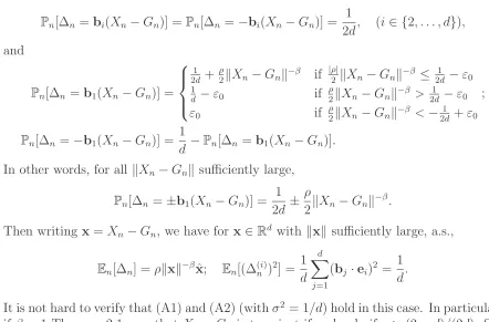
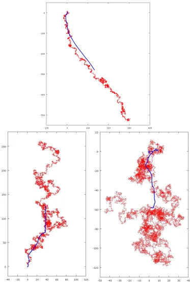
if β = 1 Theorem 2.1 says that Xn−Gn is transient if and only if ρ >(2−d)/(2d). See

Figure 2 for some simulations of this model.

Example 2. Here is another example satisfying (A1) and (A2), this time with jumps supported on a unit sphere rather than being restricted to a finite set of possibilities. Let

β >0 andρ∈R_{. Given Fn and Xn−Gn=x, the jump ∆n is obtained as follows.}

(i) ChooseUn uniformly distributed on the unit sphere Sd.

(ii) Take ∆n=Un+ρkxk−β1{ρkxk−β<1/2}xˆ.

So the jumps of the walk are uniform on a sphere, but the centre of the sphere is (forkxk

large enough) shifted slightly in the direction±xˆ, depending on the sign ofρ. Conditions (A1) and (A2) (again with σ2 _{= 1/d) are readily verified for this example.}

Example 3. We sketch one more example with d ≥ 2, β > 0 and ρ > 0, which is reminiscent of the walk avoiding its convex hull. Take the jump ∆nuniform on Sdminus

the circular cap of relative surfaceρkXn−Gnk−β pointing towards the barycentre, i.e.,

∆n is uniform on

y∈S_{d :y·xˆ >−1 +C(ρ)kxk}−β/(d−1) _,

with x=Xn−Gn, where C(ρ) is a constant depending onρand d. Here we assumekxk

Figure 2: Simulation of 104_{steps of the random walk and its centre of mass (thick line), as}

described in Example 1, withd= 2, ρ= 0.1,ε0 = 0.01, and different values of β ∈(0,1];

the three pictures have β = 0.1 (top), β = 0.5 (bottom left), and β = 1 (bottom right). Theorem 2.2 shows that in the two β < 1 cases, the random walk Xn is transient with

a limiting direction. In the β = 1 case, we know from Theorem 2.1 that Xn−Gn is

2.4

Open problems and paper outline

Our results give a detailed recurrence classification (Theorem 2.1) for the processXn−Gn.

Of considerable interest is the asymptotic behaviour of Xn itself, for which we have a

complete picture only in the case β ∈[0,1), ρ >0 (Theorem 2.2). We conjecture:

• kXnk → ∞ a.s. if and only if kXn−Gnk → ∞ a.s..

Theorems 2.2 and 2.3 verify the ‘if’ part of the conjecture when (i) β ∈[0,1) and ρ >0, and (ii) d= 1. Another open problem involves the angular behaviour of our model when

β ≥ 1. By analogy with [27] we suspect that there is no limiting direction in that case (in contrast to Theorem 2.2).

The remainder of the paper is arranged as follows. In Section 3 we describe in more detail how our model is related to Lamperti’s problem (Section 3.1), and to the centre-of-mass of SRW (Section 3.2), and we prove Theorem 1.1. We also outline the motivation of our random walk as a model for a random polymer in solution (Section 3.3). Section 4 is devoted to preliminary computations for the processesXn, Gn, and (especially)Xn−Gn.

In Section 5 we take a somewhat more general view, and study the asymptotic properties of one-dimensional, not necessarily Markov, processes satisfying a precise version of (1.4). The recurrence classification is a time-varying, more complicated analogue of Lamperti’s results [21, 23], and we use some martingale ideas related to those in [12, 31]. In the case

β ∈[0,1), ρ >0 we prove a law of large numbers that is a cornerstone of our subsequent analysis for the random walkXn. This law of large numbers is an analogue of that in [31]

for the supercritical Lamperti problem. While the results of [31] supply an upper bound crucial to our approach, the law of large numbers in the present setting requires a new idea, and our key tool here is a stochastic approximation lemma (Lemma 5.1), which may be of independent interest. Section 6 is devoted to the proofs of our main theorems. The basic method is an application of the results of Section 5 to the processkXn−Gnk, armed

with our computations in Section 4. We carry out this approach to prove Theorems 2.1 and 2.3 in Section 6.1. A crucial ingredient is the proof, in Section 6.2, thatXn−Gnhas

a limiting direction. This enables us to prove Theorem 2.2. Finally, in Section 6.3, we prove Theorem 2.4, building on some general results from [29].

3

Connections and further motivation

3.1

Lamperti’s problem and simple random walk norms

Our problem is related to a time-dependent version of the so-called Lamperti problem. We briefly review the latter here. LetZ = (Zn)n∈N be a discrete-time stochastic process

adapted to a filtration (Fn)n∈N and taking values in an unbounded subset S of [0,∞).

The set S may be countable (as in the SRW example which follows in this section) or uncountable (as in the application to stochastic billiards described in [29]).

Lamperti [21–23] investigated the extent to which the asymptotic behaviour of Z

is determined by the increment moments E_{n[(Zn+1 −Zn)}k_{] when viewed as (random)}

functions of Zn. Formally, suppose that for some k, En[(Zn+1 −Zn)k] is well-defined for

alln. Then by standard properties of conditional expectations (see e.g. [8, Section 9.1]), there exist a Borel-measurable function φk(n;·) and an Fn-measurable random variable

ψk(n) (orthogonal to Zn) such that, a.s.,

Define

µk(n;x) :=φk(n;x) +ψk(n). (3.1)

The µk(n;x) are, in general, Fn-measurable random variables; if Z is a Markov process

then µk(n;x) = E[(Zn+1 −Zn)k | Zn = x] is a deterministic function of x and n, and

if in addition Z is time-homogeneous, µk(n;x) = µk(x) is a function of x only. For

many applications, including those described here, Z will not be time-homogeneous or Markovian, but nevertheless theµk(n;x) are well-behaved asymptotically.

In this section, X = (Xn)n∈N will be the symmetric SRW on Zd (d ∈ N). That

is, X has i.i.d. increments ∆n := Xn+1 −Xn such that if {e1, . . . ,ed} is the standard

orthonormal basis on Rd_{, for i∈ {1, . . . , d},} P_{[∆n=ei] =}P_{[∆n =−ei] = (2d)}−1_.

Let Fn = σ(X1, . . . , Xn) and consider the (Fn)n∈N-adapted process Z = (Zn)n∈N on

[0,∞) defined by Zn = kXnk. Here Z takes values in the countable set S = {kxk : x∈

Zd_{}. Note that Z is not in general a Markov process: when d= 2, given one of the two}

Fn-events {Xn = (5,0)} and {Xn = (3,4)} we have Zn = 5 in each case but Zn+1 has

two different distributions; for instance Zn+1 can take the value 6 (with probability 1/4)

in the first case, but this is impossible in the second case.

We recall some simple facts about ∆n=Xn+1−Xn in the case of SRW. We have

P_{n[k∆nk ≤1] = 1, a.s., and} E_{n[∆n] =0, a.s.. (3.2)}

Writing ∆n= (∆(1)n , . . . ,∆(nd)) in Cartesian components, we have that

E_n[∆(i)

n ∆(nj)] =

1

d1{i=j}, a.s.. (3.3)

Elementary calculations based on Taylor’s expansion and (3.2) and (3.3) show that

E_{n[Zn+1−Zn] =} 1

2d

d

X

i=1

(kXn+eik+kXn−eik −2kXnk)

= 1 2kXnk

1− 1

d

+O(kXnk−2);

in the above notation,µ1(n;x) = ₂1_x(1−_d1)+O(x−2) asx→ ∞. As before, this asymptotic

expression is the compact notation for

sup

n∈N

ess supµ1(n;x) =

1 2x

1− 1

d

+O(x−2),

together with the same expression with ‘inf’ instead of each ‘sup’. Similarly

E_n[Z2

n+1−Zn2] =

1 2d

d

X

i=1

kXn+eik2+kXn−eik2−2kXnk2

= 1.

Then since (Zn+1−Zn)2 =Zn2+1−Zn2−2Zn(Zn+1−Zn) we obtain

E_{n[(Zn+1−Zn)}2_{] =} 1

d +O(kXnk

−1_).

3.2

Centre of mass for simple random walk

We saw in Section 3.1 how a mean drift described loosely by (1.3) arises from the process of norms of symmetric SRW. In this section we describe how a process with mean drift of the form (1.4) arises when considering the distance of a symmetric SRW to its centre of mass. The motion of the centre of mass of a random walk is of interest from a physical point of view, when, for example, the walk represents a growing polymer molecule: see e.g. [1] and [37], especially Chapter 6.

The centre-of-mass process (defined by (1.1)) corresponding to a symmetric SRW on

Zd _{was studied by Grill [15], who showed that the process (G}

n)n∈N returns to a fixed ball

containing the origin with probability 1 if and only if d= 1. In particular the process is transient for d≥2 and Grill gives a sharp integral test for the rate of escape of the lower envelope. A consequence of his result is the following.

Theorem 3.1. [15] Let(Xn)n∈Nbe symmetric SRW onZdand(Gn)n∈Nthe corresponding centre-of-mass process defined by (1.1). Let d∈ {2,3,4, . . .}. Then for any ε >0,

kGnk ≥(logn)−

1

d−1−εn1/2, a.s.,

for all but finitely many n∈N_{. On the other hand, for infinitely many n∈}N_,

kGnk ≤(logn)−

1

d−1n1/2, a.s..

A crude upper bound for kGnk, obtained by applying the triangle inequality kGnk ≤

1

n

Pn

i=1kXik and the law of the iterated logarithm for symmetric SRW on Zd (d∈N) to

each kXik (see e.g. Theorem 19.1 of [35]), is that for any ε >0, a.s.,

kGnk ≤

2

3d1/2(1 +ε)(2nlog logn) 1/2_,

for all but finitely many n ∈ N_{; it seems likely that this is an overestimate. In d = 1,}

in the analogous continuous setting, a result of Watanabe [38, Corollary 1, p. 237] says that, for Bt standard Brownian motion, for any ε >0, for all t large enough,

1

t Z t

0

Bsds≤3−1/2(1 +ε)(2tlog logt)1/2, a.s.,

and this bound is sharp in that the inequality fails infinitely often, a.s., when ε = 0. Standard strong approximation results show that this result can be transferred to kGtk

ind = 1.

The next result shows how the drift equation (1.4) arises in this context. Lemma 3.1 is a consequence of the more general Lemma 4.2 below.

Lemma 3.1. Let d∈N_{. Suppose that(Xn)n∈}N is a symmetric SRW on Zd, and(G_n)_n∈N is its centre-of-mass process as defined by (1.1). Let Fn := σ(X1, . . . , Xn) and Yn :=

Xn−Gn. Then, a.s.,

E_{n[kYn+1k − kYnk] =}

1− 1

d

1 2kYnk

− kYnk

n+ 1 +O(kYnk

−2_);

E_{n[(kYn+1k − kYnk)}2_{] =} 1

d +O(kYnkn

−1_{) +O(kY}

Neglecting higher-order terms, the study of the process kXn−Gnk for SRW leads

to the analysis of a process with drift given by (1.4). Lemma 3.1 can be generalized to zero-drift Markov chainsX = (Xn)n∈N satisfying appropriate versions of (3.2) and (3.3).

We prove our results on SRW by applying our general results given in Sections 4 and 5.

Proof of Lemma 3.1. This follows from Lemma 4.2 stated and proved in Section 4. Ta-king expectations in (4.10) and using (3.2) and (3.3) we obtain the first equation in the statement of the lemma, using the fact that kYnk=o(n) a.s. to simplify the error terms.

Similarly, squaring both sides of (4.10) and taking expectations we obtain the second equation in the lemma.

Proof of Theorem 1.1. Let Zn =kYnk =kXn−Gnk and Fn =σ(X1, . . . , Xn). Then by

Lemma 3.1, a.s.,

E_{n[Zn+1−Zn] =}

1− 1

d

1 2Zn

− Zn

n +O(n

−2_Z

n) +O(Zn−2);

E_{n[(Zn+1−Zn)}2_{] =} 1

d+O(Znn

−1_{) +O(Z}−1

n ).

Thus (5.4) and (5.5) hold withρ′ _{= (d−1)/(2d) and σ}2 _{= 1/d. It follows from Theorems}

5.1 and 5.2 (stated and proved in Section 5) that Zn is transient if and only if 2ρ′ > σ2,

or equivalently 1−(1/d)>(1/d), that is, d >2.

3.3

The process viewed as a new random polymer model

In this section we briefly summarize motivation of self-interacting random walks arising from polymer physics, and give an interpretation of our model described by (A1) in that context. Much more background is provided by, for instance, [28, Section 2.2], [37, Chapter 7], [17, Chapter 7], and, for the underlying physics, [36]. Recent accounts of some of the relevant probability theory are given in [14, 16].

The sites visited by the walkXnrepresent the monomers that make up a long polymer

molecule in solution inRd_{(of course, physicallyd∈ {2,3}are most interesting). The line}

segments between successive sitesXn andXn+1 represent the chemical bonds holding the

molecule together; in this regard our condition of uniformly bounded increments in (A1) is natural. We assume that the polymer solution is dilute, so that interaction between different polymer molecules can be neglected.

In real polymers, a phase transition is observed between polymers in poor solvents(or at low temperature) and good solvents (or high temperature) [36, Chapter 7]. In poor solvents, a polymer molecule collapses as the attraction between monomers overcomes the excluded volume effect caused by the fact that no two monomers can occupy the same physical space. In good solvents, a polymer molecule exists in an extended phase where the excluded volume effect dominates.

It is the extended phase that is believed to lie in the same universality class as SAW. Heuristic arguments dating back to P.J. Flory (see e.g. [28, Section 2.2]) suggest that in this phase kXnk should exist on ‘macroscopic scale’ of order nν for an exponent ν =

ν(d) ∈ [1/2,1], with ν < 1 for d > 1 and ν > 1/2 for d ≤ 3. So for d ∈ {2,3}, the polymer is expected to be super-diffusive but sub-ballistic. According to Theorem 2.4(i), our model defined by (A1) has macroscopic scale exponent max{1/2,1/(1 +β)} when

dominates. For instance, since ν(2) = 3/4, in d = 2 the ‘physical’ choice of our model has β = 1/3 and ρ > 0; it is not clear to what extent that case of our model replicates the behaviour of SAW.

On the other hand, the collapsed phase corresponds to taking ρ < 0 in (A1), where the polymer’s self-attraction, summarized through its centre of mass, is dominant. See Theorem 2.4(iii) and (iv). Between the poor and good solvent phases, there is a transitio-nal phase at the so-called θ-point at which the temperature achieves a specific (critical) value T =θ. Here the excluded volume effect and self-attraction are in balance, and the molecule behaves rather like a simple random walk path. Compare Theorem 2.4(ii).

4

Properties of the self-interacting random walk

Under the assumption (A1), we are going to study the processXn−Gnand in particular

determine whether it is transient or recurrent. It suffices to study kXn−Gnk. In this

section we analyse the basic properties of the latter process; subsequently we will apply our general results of Section 5 on processes that satisfy, roughly speaking, (1.4).

We introduce some convenient notation that we use throughout. For n∈N _set

Yn :=Xn−Gn, ∆n:=Xn+1−Xn.

We start with some elementary relations amongst Xn,Gn, and Yn following from (1.1).

Lemma 4.1. Suppose that (Xn)n∈N is a stochastic process on Rd, and (G_n)_n∈N is its centre-of-mass process as defined by (1.1). For n ∈N _{we have}

Gn+1 =

n

n+ 1Gn+ 1

n+ 1Xn+1; and (4.1)

Yn+1 =

n

n+ 1(Yn+ ∆n). (4.2)

Moreover G1 =X1 and for n∈ {2,3, . . .},

Gn =X1+

n

X

j=2

1

j−1Yj. (4.3)

Proof. Equation (4.1) is immediate from (1.1). Then from (4.1) we have that for n∈N_,

Yn+1 =Xn+1−Gn+1 =

n

n+ 1 (Xn+1−Gn), (4.4)

from which (4.2) follows since Xn+1−Gn=Yn+ ∆n. For (4.3), we have from (4.1) again

that for n∈N_,

Gn+1−Gn=

1

n+ 1(Xn+1−Gn) = 1

nYn+1,

where the final equality is obtained from (4.4). Thus for n ≥2,

Gn−G1 =

n−1

X

j=1

(Gj+1−Gj) = n−1

X

j=1

1

jYj+1,

The main result of this section concerns the increments of the process kYnk under

assumption (A1) and also possibly (A2). Part (i) of Proposition 4.1 gives basic regularity properties, including boundedness of jumps. Part (ii) gives an expression for the mean drift when β ∈[0,1). Part (iii) deals with the caseβ ≥1 when (A2) also holds.

Proposition 4.1. Suppose that (A1) holds.

(i) There exists C ∈(0,∞) for which, for any n∈N_,

P_{n[|kYn+1k − kYnk|> C] = 0, a.s.. (4.5)}

In addition

lim sup

n→∞

kYnk=∞, a.s.. (4.6)

(ii) If β ∈[0,1) then, a.s.,

E_{n[kYn+1k − kYnk] =ρkYnk}−β ₋ kYnk

n+ 1 +O(kYnk

−β_(logkY

nk)−2). (4.7)

(iii) Suppose also that (A2) holds and β ≥1. Then, a.s.,

E_{n[kYn+1k − kYnk] =}

ρ1{β=1} +

1

2(d−1)σ

2

kYnk−1−

kYnk

n+ 1

+o(kYnk−1(logkYnk)−1); (4.8)

E_{n[(kYn+1k − kYnk)}2_{] =σ}2_+O(n−1_{kYnk) +o((logkYnk)}−1_{). (4.9)}

We prove Proposition 4.1 via a series of lemmas. The first gives information on the increments of the process given by the distance of a general stochastic process to its centre-of-mass. In particular, it shows thatkYnkinherits boundedness of jumps fromXn,

and gives an expression for the increments ofkYnkin terms of ∆n, the increments of Xn.

Lemma 4.2. Suppose that (Xn)n∈N is a stochastic process on Rd, and (Gn)n∈N is its centre-of-mass process as defined by (1.1). Suppose that X1 ∈ Rd is fixed and that (2.1)

holds for some B ∈(0,∞). There existsC ∈(0,∞)for which, for alln ∈N_{, (4.5) holds.}

Moreover, a.s.,

kYn+1k − kYnk=

n n+ 1

Yn·∆n

kYnk

+k∆nk

2

2kYnk

− (Yn·∆n) 2

2kYnk3

+O(kYnk−2)−

kYnk

n+ 1. (4.10)

Proof. We work with the process (kYnk)n∈N. From (2.1) and the triangle inequality, we

have the simple bound kXnk ≤ kX1k+B(n−1) a.s., for alln∈N. Applying the triangle

inequality in (1.1) then yields the equally simple bound

kGnk ≤

1

n

n

X

i=1

(kX1k+B(i−1)) ≤ kX1k+

Bn

2 .

Combining these two inequalities together with the fact that kYnk ≤ kXnk+kGnk, it

follows thatkYnk ≤2kX1k+(3Bn/2) a.s., for alln ∈N. Then from the triangle inequality

and (4.2) we have that

|kYn+1k − kYnk| ≤ kYn+1−Ynk ≤

1

nkYnk+k∆nk ≤

5B

2 +

2kX1k

a.s., by (2.1), and this lattermost quantity is uniformly bounded. Thus we have (4.5). For the final statement of the lemma, note that, from (4.2),

kYn+1k=

n

n+ 1 kYnk

2_+k∆

nk2+ 2Yn·∆n

1/2

. (4.11)

Now writingy=Yn for convenience, we obtain from (4.11) that

kYn+1k − kYnk=kyk

" n n+ 1

1 + k∆nk

2_{+ 2y·∆}

n

kyk2

1/2

−1

#

. (4.12)

Using Taylor’s formula for (1 +x)1/2 _{with Lagrange remainder in (4.12) implies that}

kYn+1k − kYnk=

nkyk

n+ 1

k∆nk2+ 2y·∆n

2kyk2 −

(k∆nk2+ 2y·∆n)2

8kyk4 +O(kyk −3₎

− kyk

n+ 1,

using (2.1) for the error bound. Simplifying and again using (2.1), this becomes

kYn+1k − kYnk=

nkyk

n+ 1

k∆nk2

2kyk2 +

y·∆n

kyk2 −

(y·∆n)2

2kyk4 +O(kyk −3₎

− kyk

n+ 1.

Then equation (4.10) follows.

Now we turn to the model defined by (A1), starting with the drift of kYnk. For

a, b∈R_{, we use the standard notation a∧b := min{a, b}.}

Lemma 4.3. Suppose that (A1) holds. Then the drift of kYnk satisfies, a.s.,

E_{n[kYn+1k − kYnk] =} n

n+ 1 ρkYnk

−β _{+ Θ}

nkYnk−1

− kYnk

n+ 1

+O(kYnk−(1∧β)(logkYnk)−2), (4.13)

where Θn is the Fn-measurable random variable given by

Θn =

1 2kYnk

−2_E

n[kYnk2k∆nk2−(Yn·∆n)2]. (4.14)

Moreover, there exists C < ∞ such that Θn ∈[0, C] a.s., and if β ∈[0,1), (4.7) holds.

Proof. Taking expectations in (4.10), using the fact that

kYnk−1En[Yn·∆n] =ρkYnk−β +O(kYnk−β(logkYnk)−2),

by (2.2), we obtain

E_{n[kYn+1k − kYnk] =} n n+ 1

ρkYnk−β +

1 2kYnk3

E_n[kYnk2_k∆nk2_{−(Yn·∆n)}2_]

+O(kYnk−(β∧1)(logkYnk)−2)−

kYnk

n+ 1.

By the fact that|Yn·∆n| ≤ kYnkk∆nkand the jumps bound (2.1) we have that

0≤E_n[kYnk2_k∆nk2_{−(Yn·∆n)}2_]≤CkYnk2_{, a.s.,}

for some C ∈ (0,∞). Thus defining Θn by (4.14) we obtain (4.13) and the fact that

The next result shows how the ellipticity condition (2.3) leads to (4.6).

Lemma 4.4. Suppose that (A1) holds. Then lim supn→∞kYnk=∞ a.s..

Proof. We have from (4.11) that

kYn+1k2− kYnk2 =

n n+ 1

2

k∆nk2+ 2Yn·∆n

− 2n+ 1

(n+ 1)2kYnk

2_{. (4.15)}

Fix p ∈ N_{, and define Fn,1 := ∩}np+(p−1)

i=np {∆i·Yˆi ≥ ε0} and Fn,2 := {kYnpk ≤ ε0₁₆np}. Fix

also np ∈Nwith ε0np ≥16C, whereC is as in (4.5), and consider n≥np only. By (2.3)

we have thatP_n[Fn,1]≥εp

0 a.s., and hence L´evy’s extension of the second Borel–Cantelli

lemma (see e.g. [10, Theorem 5.3.2]) implies that P_{[Fn,1 i.o.] = 1.}

Now, observe from (4.5) that kYi+1k ≤ kYik+C, a.s., which implies on Fn,2 that kYik ≤ 1₈ε0np for alli∈ {np, . . . np+ (p−1)}. Then, onFn,1∩Fn,2, we obtain from (4.15)

that, a.s.,

kYi+1k2− kYik2 ≥ −

2

ikYik

2₊1

4 ε

2

0+ 2ε0kYik

≥ 1

4ε0kYik+ 1 4ε

2 0 ≥

1 4ε

2 0,

for any i with np≤i≤np+ (p−1) and any n ≥np. Hence on Fn,1∩Fn,2, a.s.,

kY(n+1)pk2 =kYnpk2+

np+(p−1)

X

i=np

(kYi+1k2− kYik2)≥pε20/4.

Thus, up to sets of probability zero, {(Fn,1∩Fn,2) i.o.} ⊆ {lim supn→∞kYnk ≥p1/2ε0/2}.

Moreover, by definition ofFn,2,{Fn,c2 i.o.} ⊆ {lim supn→∞kYnk=∞}. Since{Fn,1 i.o.} ⊆ {(Fn,1∩Fn,2) i.o.}∪ {Fn,c2 i.o}, it follows that{Fn,1 i.o.} ⊆ {lim supn→∞kYnk ≥p1/2ε0/2}.

Since p was arbitrary, the result follows from the fact that P_{[Fn,1 i.o.] = 1, as shown in}

the first part of this proof.

When (A1) holds with β ≥ 1, we need more regularity to obtain a well-behaved version of (4.13). Thus we impose (A2) and use the following result, which in addition gives an expression for the second moment of the increment kYn+1k − kYnk.

Lemma 4.5. Suppose that (A1) and (A2) hold. Then Θn as defined by (4.14) satisfies

Θn =

1

2(d−1)σ

2_+o((logkY

nk)−1), a.s.. (4.16)

Moreover, (4.9) holds.

Proof. First we prove (4.16). We have that

E_n[k∆nk2_{] =}

d

X

i=1

E_n[(∆(i)

n )2] =dσ2 +o((logkYnk)−1),

by (2.5). Also if Yn= (y1, . . . , yd)∈Rd, with the convention that an empty sum is 0,

E_n[(Yn·∆n)2_{] =}

d

X

i=1

y_i2E_n[(∆(i)

n )2] + 2 d

X

i=2

i−1

X

j=1

=kYnk2

σ2+o((logkYnk)−1)

, (4.17)

by (2.5) and (2.6). Then (4.16) follows from (4.14).

Next we prove (4.9). Squaring both sides of (4.10) and taking expectations we obtain

E_{n[(kYn+1k − kYnk)}2_{] =kYnk}−2E_n[(Yn·∆n)2_{] +O(n}−1_{kYnk) +O(kYnk}−1_).

Now using (4.17) yields (4.9).

Proof of Proposition 4.1. We collect results from Lemmas 4.2, 4.3, 4.4, and 4.5.

5

Recurrence classification for processes satisfying

equation (1.4)

5.1

Introduction

In this section we state general results for processes with drift of the form (1.4). We will later apply these results to the processkXn−Gnksatisfying (A1) (and maybe also (A2)),

but for this section we work in some generality.

Let (Zn)n∈N be a stochastic process taking values in an unbounded subsetS of [0,∞),

adapted to a filtration (Fn)n∈N. Recall the definition of µk(n;x) from (3.1), so that

E_{n[(Zn+1−Zn)}k_{] =µk(n;Zn) a.s.. As discussed in Section 3.1, the case whereµ2(n;x) is} O(1) andµ1(n;x)→0 asx→ ∞arises often in applications; the case whereµ1(n;x)→0

uniformly inn is sometimes known as Lamperti’s problem after Lamperti’s work [21–23]. Roughly speaking, the Lamperti problem has µ1(n;x) ≈ ρx−β, β > 0, ρ ∈ R, ignoring

higher-order terms. Results of Lamperti [21,23] imply that the caseβ = 1 is critical from the point of view of the recurrence classification. The supercritical case, when β ∈[0,1),

ρ >0, has also been studied (see [31] and references therein).

In this section we study the analogous problem for whichµ1(n;x)≈ρx−β−(x/n). In

keeping with the applications of the present paper, and to ease technical difficulties, we adopt some stronger regularity assumptions than imposed in [21,23] or [31]. Nevertheless, this version of the problem is more difficult than the classical case (without the extra−x/n

term in the drift). Thus although the ideas in this section are related to those in [21, 23] and [31], we have to proceed somewhat differently. In particular, to obtain our β < 1 law of large numbers in this setting (an analogue of [31, Theorem 2.3] for the standard Lamperti case), we use a ‘stochastic approximation’ result (Lemma 5.1), the proof of which uses ideas somewhat similar to those in [30, 31].

We impose some regularity conditions on (Zn)n∈N. Suppose that there exists C ∈

(0,∞) such that for all n∈N_,

P_{n[|Zn+1−Zn|> C] = 0, a.s.. (5.1)}

We also assume that

lim sup

n→∞ Zn =∞, a.s., (5.2)

without which the question of whether (Zn)n∈N is recurrent or transient (in the sense of

Definition 2.1) is trivial. Note that (5.2) is implied by a suitable ‘irreducibility’ assump-tion, such as, for ally >0, infn∈NP_n[Z_m−Z_n > y for some m > n]>0, a.s.. In our case,

5.2

The critical case:

β

= 1

Forx >0 and n∈N _define

r(n;x) := n−1_x2_{+ (log(1 +x))}−1_{. (5.3)}

For p > 0 we write logpx for (logx)p_{. We impose the further assumptions that there}

exist ρ′ _{∈R and s}2 _{∈(0,∞) such that}

µ1(n;x) =ρ′x−1−

x n +o(x

−1_{r(n;x)), (5.4)}

µ2(n;x) =s2+o(r(n;x)). (5.5)

Theorem 5.1. Suppose that the process (Zn)n∈N satisfies (5.1), (5.2), (5.4) and (5.5) for some ρ′ _{∈R and s}2 _{∈(0,∞). Then if 2ρ}′ _≤s2_{, Z}

n is recurrent.

Proof. Let Wn := log logZn. Write Dn := Zn+1 −Zn. First note that Taylor’s formula

implies that forx, h with x→ ∞ and h=o(x/logx),

log log(x+h) = log logx+ h

xlogx −

(logx+ 1)h2

2x2_log2_x +O(h

3_x−3_(logx)−1_).

Settingx=Zn and h=Dn and then taking expectations, we obtain

E_{n[Wn+1−Wn] =} µ1(n;Zn) ZnlogZn

− (logZn+ 1)µ2(n;Zn)

2Z2

nlog2Zn

+O(Z_n−3),

using (5.1) for the error term. By (5.4) and (5.5) this last expression is

2ρ′_−s2

2Z2

nlogZn

− s

2

2Z2

nlog2Zn

− 1

nlogZn

+o(Z_n−2(logZn)−1r(n;Zn))<0,

for all n and Zn large enough, provided 2ρ′ −s2 ≤ 0, by (5.3). Thus there exist

non-random constants w0 ∈(0,∞) and n1 ∈N for which, for all n ≥n1, on {Wn> w0},

E_{n[Wn+1−Wn]<0, a.s..}

By Doob’s decomposition, we may write Wn =Mn+An, n ≥n1, whereWn1 =Mn1, (Mn)n≥n1 is a martingale, and the previsible sequence (An)n≥n1 is defined by

An = n−1

X

m=n1

E_{m[Wm+1−Wm]≤}

n−1

X

m=n1

E_{m[Wm+1−Wm]1{Wm ≤w0} ≤C}

n−1

X

m=n1

1{Wm≤w0},

since the uniform jumps bound (5.1) for Zn implies a uniform jumps bound for Wn,

n ≥ n1. Hence Wn → ∞ implies that lim supn→∞An <∞ so Mn → ∞ also. However,

(Mn)n≥n1 is a martingale with uniformly bounded increments (by (5.1)) soP[Mn → ∞] = 0 (see e.g. [10, Theorem 5.3.1, p. 204]). Hence P_{[lim infn→∞Wn <∞] = 1.}

Theorem 5.2. Suppose that the process (Zn)n∈N satisfies (5.1), (5.2), (5.4) and (5.5) for some ρ′ _{∈R and s}2 _{∈(0,∞). Then if 2ρ}′ _{> s}2_{, Z}

Proof. This time set

Wn :=

1 logZn

+ 9 logn.

Again write Dn:=Zn+1−Zn. We want to compute

E_{n[Wn+1−Wn] =}E_n

(log(Zn+Dn))−1−(logZn)−1

+ 9

(log(n+ 1))−1−(logn)−1

. (5.6)

Observe that, for the final term on the right-hand side of (5.6),

(log(n+ 1))−1−(logn)−1 = log(1−(n+ 1)

−1₎

lognlog(n+ 1) =− 1

nlog2n +O(n

−2_{). (5.7)}

Also for the expectation on the right-hand side of (5.6) we have that

E_{n(log(Zn+Dn))}−1_−(logZn)−1

= (logZn)−1En

"

1 + log(1 + (Dn/Zn)) logZn

−1

−1

#

.

Taylor’s formula implies that for a=O(1) andy=o(1),

(1 +alog(1 +y))−1 = 1−ay+ 2a

2_+a

2 y

2_+O(y3_).

Applying this formula with a= 1/logZn and y=Dn/Zn we obtain,

E_{n(log(Zn+Dn))}−1_−(logZn)−1

=−µ1(n;Zn)

Znlog2Zn

+ µ2(n;Zn) 2Z2

nlog2Zn

+ µ2(n;Zn)

Z2

nlog3Zn

+O(Z_n−3),

by (5.1). Now using (5.4) and (5.5) we obtain,

E_{n(log(Zn+Dn))}−1_−(logZn)−1

= 1

2Z2

nlog2Zn

−(2ρ′−s2) +o(r(n;Zn)) +O((logZn)−1)

+ 1

nlog2Zn

. (5.8)

Suppose that 2ρ′ _−s2 _{≥ 2ε > 0. Then by (5.3), (5.6), (5.7) and (5.8) we have that}

there exist non-random constants n0 ∈ N and x0 ∈ (1,∞) such that for all n ≥ n0, on {Zn≥x0}, a.s.,

E_{n[Wn+1−Wn]≤ −} ε

2Z2

nlog2Zn

− 8

nlog2n +

3 2nlog2Zn

. (5.9)

We have that the right-hand side of (5.9) is bounded above by

1 log2Zn

−ε

2Z2

n

+ 3 2n

≤ 1

log2Zn

−ε

2Z2

n

+ 3ε 8Z2

n

,

provided n ≥ 4Z2

nε−1, and this last upper bound is negative for Zn ≥ x0. On the other

hand, if n≤4Z2

nε−1 the right-hand side of (5.9) is bounded above by

1

n

3/2 log2Zn

− 8

log2n

≤ 1

n

7 log2n −

8 log2n

for Zn ≥x0 and n ≥n0. Thus in either case we have concluded that for all n ≥n0, on {Zn≥x0},

E_{n[Wn+1−Wn]<0, a.s.. (5.10)}

Now fix K >1 and x1 ≥x0. Define the stopping times

σK := min{n ≥max{n0, x118K}:Zn≥x14K}; τK := min{n≥σK :Zn ≤x1}.

By (5.2) we have thatP_{[σK <∞] = 1. From (5.10) and the definition ofτK we have that}

(Wn∧τK)n≥σK is a non-negative supermartingale, and hence it converges almost surely to

a [0,∞)-valued random variable W :=W(K)_{. In particular, since σ}

K <∞ a.s., we have

limn→∞Wn∧τK =W, a.s.. Moreover

E_[W]≥E_[W1{τ

K<∞}] =E[WτK1{τK<∞}]≥

P_{[τK <∞]}

logx1

, (5.11)

since ZτK ≤x1. On the other hand, since (Wn∧τK)n≥σK is a supermartingale,

E_[W]≤E_[Wσ

K]≤

1 4Klogx1

+ 9

18Klogx1

= 3

4Klogx1

, (5.12)

using the facts thatZσK ≥x

4K

1 andσK ≥x181 K. Combining (5.11) and (5.12) we see that

P_{[τK <∞]}

logx1

≤ 3

4Klogx1

.

On{σK <∞} ∩ {τK =∞}, we have that lim infn→∞Zn ≥x1, so the preceding argument

shows that P_{[lim infn→∞Zn ≥x1] ≥ 1−} 3

4K for anyK and any x1 ≥x0. It follows that

P_{[Zn→ ∞] = 1.}

5.3

The supercritical case:

β

∈

[0

,

1)

Once again we will assume that (5.1) and (5.2) hold. We will also assume that there exist

β ∈[0,1) and ρ∈R_{\ {0}such that}

µ1(n;x) =ρx−β −

x n +o(x

−β_{) +o(xn}−1_{). (5.13)}

Theorem 5.3. Consider the process (Zn)n∈N satisfying (5.1), (5.2), and (5.13), where

β ∈[0,1). Then Zn is transient if ρ >0 and recurrent if ρ <0.

Proof. First suppose that ρ >0. By (5.1) we can choose ρ′ _{∈(0,∞) so that 2ρ}′ _{> C}2 _>

E_{n[(Zn+1−Zn)}2_{], a.s., and, by (5.13),}

E_{n[Zn+1−Zn]≥(ρ}′_+o(1))Z−1

n −

Zn

n +o(Z

−1

n r(n;Zn)), a.s..

It is this inequality, rather than the equality (5.4), that is needed in the proof of Theorem 5.2. Hence following that proof implies transience. Similarly, if ρ < 0 we have, for any

ρ′ _{∈(−∞,0), a.s.,}

E_{n[Zn+1−Zn]≤(ρ}′_+o(1))Z−1

n −

Zn

n +o(Z

−1

n r(n;Zn)).