Abstract: In the field of Array Signal Processing, the problem of Direction of Arrival (DOA) estimation has attracted colossal attention of researchers in the past few years. The problem refers to estimating the angle of arrival of the incoming signals at the receiver end, from the knowledge of the received signal itself. Generally, an array of antenna/sensors is employed at the receiver for this purpose. In over-determined DOA estimation, the number of signal sources, whose direction needs to be estimated are usually lesser than half the number of antenna array elements, whereas the challenge is to estimate the DOAs in under-determined case, where the signal source number is quiet larger than the number of antenna array elements. This paper tackles such a problem by the application of multiple level nested array. Instead of subspace-based techniques for the estimation, sparse signal representation for Compressive Sensing (CS) framework is used, which eliminates the requirement of prior information about the source number and also the tedious task of computing the inverse of the covariance matrices. In this paper, we propose an adaptive approach for Least Absolute Shrinkage and Selection Operator (LASSO) with reduced number of computations by singular value decomposing of the received signal vector. The outcomes of this paper showcase that the presented algorithm achieves high degree of freedom (DOF), good resolution, minimum root mean square error and less computational complexity with increased speed of estimation.
Index Terms: Nested Arrays, LASSO, On-grid estimation, Singular Value Decomposition, Sparse Signal Representation, Underdetermined-Direction of Arrival estimation.
I. INTRODUCTION
In the recent years, direction of arrival estimation has become the most addressed hot-topic of the researchers, playing a key role in several applications such as RADAR, SONAR, Seismology, wireless communication etc. There are several algorithms designed for this purpose since from the last decade including conventional beamforming, Capon beamforming [2], subspace-based estimation like MUSIC [1], ESPRIT [3] and its improved versions like I-MUSIC, R-MUSIC [4] etc. These algorithms provide good resolution and accuracy but requires the prior information about the source number. They also suffer from yielding sharp spatial spectral peaks at the actual DOAs. These algorithms exhibit better results for the overdetermined case of DOA estimation. In the recent years, after the emerge of sparse signal representation theory, the insight of solving DOA estimation problem has been and being changed with respect to compressive sensing (CS) framework. The underlying spatial
Revised Manuscript Received on September 08, 2019.
Raghu K, School of Electronics & Communication Engg, REVA
University, Bengaluru, India.
Prameela Kumari N, School of Electronics & Communication Engg,
sparsity enables one to link CS framework to angle of arrival estimation problem. The application of sparse signal reconstruction technique for DOA estimation has wider advantages such as smaller number of snapshots, lesser sensitivity over SNR, ability to deal with highly correlated or coherent sources etc, over the aforementioned traditional estimation methods. In [5], a single snapshot l1-norm minimization and its dimension reduction algorithm l1-SVD for multiple snapshot algorithm was proposed. Several applications involving DOA estimation based on CS framework has been investigated in [6]-[9]. Representing the array covariance vectors in sparse domain with error suppression criteria for DOA estimation is proposed in [10]. In [11]-[13], it has been proved that estimating DOA in underdetermined case is very difficult. For such cases, special array structures have been proposed in [14]-[17]. In recent years, nested array structures and co-prime array structures are the two sparse arrays that are proposed in [18] and [19]. By considering the nested or co-prime array structures, a virtual linear array with more number of array elements can be modelled and used for underdetermined-DOA estimation which enhances the degrees of freedom (DOFs). Spatial smoothing based sub-space approaches [20]-[22] were proposed for difference co-array structures for the underdetermined case. In [23], the underdetermined DOA estimation problem is addressed by employing signal reconstruction methods of CS framework. Furthermore in [24] and [25], super-nested arrays and higher order difference co-array structures are proposed to increase the DOFs with limited number of physical antenna array elements.
For both the classes of sparse array structures aforementioned, atleast two uniform linear sub-arrays are required to optimize the virtual array locations in correspondence to the difference co-array. The major problem faced in on-grid DOA estimation is grid mismatch. This problem is where the actual DOAs of the signal sources are not found in the defined values of finite search grid. One simple solution for this problem is to define a thicker search grid having a step size of very less value, but the algorithm‟s computational complexity increases which leads to reduced speed of estimation. The alternative solution proposed in [5] is to adapt and reframe the search grid only in and about the angle spaces where the actual signal sources are localized. Use of off-grid based DOA estimation methods can also eliminate the problem of grid mismatch [23]. This paper proposes an adaptive SVD-Least Absolute Shrinkage & Selection Operator algorithm using nested array structure for underdetermined-Direction
of Arrival estimation in the following sections.
On-grid Adaptive Compressive Sensing Framework
for Underdetermined DOA Estimation by Employing
Singular Value Decomposition
II. SIGNALMODELFOR
UNDERDETERMINED-DOAESTIMATION
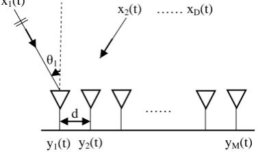
Assuming the narrowband signal case and the signal is emitted from the point source in the far-field, let us consider a uniform linear array (ULA) shown in Fig 1, which contains „M‟ number of array elements, each spaced uniformly at a distance of „d‟ between each other. Consider „D‟ number of signal sources x=[x1(n), x2(n)….xD(n)]
T
that are impinging on the ULA each with the direction of arrival θ1, θ2…. θD respectively.
Where n=1,2….K are the number of snapshots taken. Initially, let us model the problem for a single snapshot case with K=1. Let y=[y1(n), y2(n)….yM(n)]
T
be the received signal vector from the array elements, w=[w1(n), w2(n)….wM(n)]
T
be the noise vector corresponding to each array element. Representing the array received signal y in matrix form gives (1).
yAxw (1)
Where A=[a(θ1), a(θ2)…. a(θD)] is the array manifold matrix,
each of its columns a(θi) referred to as „atoms‟ corresponding to
ith signal source and given by (2).
a(θi) =[1, e-jβdsinθi , e-j2βdsinθi….. e-j(M-1)βdsinθi]T (2)
where β=2π/λ and λ stands for wavelength of the received signal, note that for a ULA dλ/2always. Let us assume the array element noise w(n) as white in spatial and temporal domains and uncorrelated with the source signals. By assuming the signal sources are also to be temporally uncorrelated with each other, the autocorrelation matrix Rxx of the signal source vector x is diagonal. The received signal vector‟s (y‟s) autocorrelation matrix is given by (3).
Where Rxx = diag(σ12, σ22….. σD2). Now vectorizing the
equation (3), we get equation (4).
Where p = [σ12, σ22….. σD2]T, iv is the vectorized form of the identity matrix and σn2 is the noise variance. By comparing
equation (4) with equation (1), z can be treated as the signal vector received by an array with manifold (A*A), where denotes the KR product. The vector p represents the signal
source vector and σn2iv represents the deterministic noise vector. The unique rows of (A*A) denotes the manifold of virtual longer array with sensors located at positions given by unique values in the set {(di-dj) for 1≤ i,j ≤ M }, where di and dj
denotes the positions of the ith and jth array elements in the original array respectively.
This virtual array formed by vectorizing the autocorrelation matrix of received signal vector y is named as difference virtual co-array of the original physical array [24].
III. NESTEDARRAYS
This section, elaborates the concept of the difference virtual co-array, its properties and the degrees of freedom (DOF) offered by the co-array. Later we discuss the specific nested array structure for the original array which yields a uniform linear difference virtual co-array.
A. Difference Co-array
Consider an array with M sensors, where the ith sensor in the array located at di position. The difference virtual co-array
of the given array has sensor positions given by the distinct values of the set { (di-dj) for 1≤ i,j ≤ M }. By cardinality of the
distinct position set of difference virtual co-array, the degrees of freedom (DOF) can be obtained. As mentioned in [25], for an array of any geometry with M sensors, the maximum DOF that can be obtained from a difference virtual co-array is given by (5)
DOFmax = M(M-1)+1 (5)
The DOF obtained is directly proportional to the source number that can be resolved using the smaller number of physical sensors. The key behind increasing the DOF of a difference virtual co-array is to use a non-uniform original physical array [25]. One such non-uniform array structure proposed by [25] can be easily obtained in a systematic method is called the “Nested Arrays” for which it is possible to obtain O(M2) degrees of freedom for the difference virtual co-array obtained from an O(M) original physical array which is a nested array.
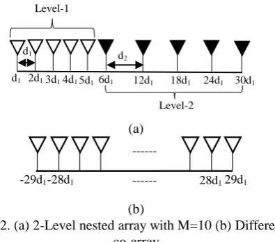
B. Level-2 Nested Array
Consider a level-2 nested array with M number of sensor elements, which is a combination of two ULA‟s: inner and outer ULA. The inner ULA consists of M1 array elements
each element spaced at a distance of d1 with its adjacent
element. The array locations of inner ULA are given by (6). The outer ULA consists of M2 array elements with an element
spacing of d2 and such that d2 = (M1+1)d1. The array locations
of outer ULA are given by (7).
Locinner = {m d1, m = 1, 2….M1} (6)
Locouter = {m d2, m = 1, 2….M2}
Locouter = {m(M1+1)d1, m = 1, 2….M2} (7)
The difference virtual co-array for this original level-2 nested array will be a filled ULA with number of virtual array elements given in (8) whose locations are given by the set in (9).
I
A
AR
R
yy
xx H
σ
n2]
[
HE
yy
R
yy
(
(
)
(
)
)
(
2)
1 2
I
a
a
R
z
yy nD
i
i H i
i
vec
σ
σ
vec
vec
(4)
v
i
p
A
A
z
(
*
)
σ
n21
)
1
(
2
2 1
M
M
M
(8)} 1 ) 1 1 ( 2 .... 1 ) 1 1 ( 2 ,
1
{
md m M M M M
cr
L (9)
θ1
x1(t) x
2(t) …… xD(t)
y1(t) y2(t) yM(t)
[image:2.595.72.261.648.759.2]d ……
Fig 1. Uniform Linear Array
Thus, we can achieve a DOF of 2M2(M1+1)-1 by considering
this level-2 nested array as the original array having only M=M1+M2 physical array elements. A level-2 nested array
with M=10 and its difference virtual co-array is shown in Fig 2. Further the DOF can be increased by increasing the number of levels of the nested array, but the resultant difference virtual co-array will no longer be a filled ULA. The number of nested levels and the number of sensor elements in each level can be estimated for a given M number of elements by maximizing the degree of freedom. This can be casted as an N-level nested array optimization problem.
IV. COMPRESSIVESENSINGFRAMEWORK
The compressive sensing (CS) framework can be applied to DOA estimation by considering the problem of estimating the direction of arrival as a problem of sparse signal reconstruction. For the sparse signal reconstruction, firstly, the approach should be discrete and secondly, the signal to be estimated must be preferably sparse in nature. In DOA estimation, the search range of angle of arrival (AOA) is actually continuous. Thus, it is necessary to discretize the continuous AOA range into a finite set. This technique is defined as DOA estimation by on-grid approach. The signal sources become sparse in spatial domain by assuming them as far-field signal sources.
A. Least Absolute Shrinkage & Selection Operator (LASSO) for Multiple Snapshot
Let us consider a finite grid of length N and the possible DOAs in the search grid is given by the set Ω = {θn}n=1 to N and
manifold of the physical array is A=[a(θ1), a(θ2)…. a(θN)].
Considering a multiple snapshot signal model for underdetermined DOA estimation with K number of snapshots and re-representing the equation (4) as:
Where, Z ϵ CMsxK represents the received signal from the virtual array, Ã=(A*A) ϵ CMsxN array manifold of the virtual difference co-array, P ϵ CNxK is the received signal power as a function of the source location and Nw ϵ CMsxK is the sensor noise matrix with Ms=M2 number of virtual elements of the
difference virtual co-array.
The methodology of DOA estimation involves estimating the signal power P as a function of all the possible DOA points, the angle points for which the signal power shows peaks are the actual signal source locations. As the sources are assumed to be
point sources the spatial spectrum is sparse. Therefore, one such sparse solution for the problem in (10) is given by ℓ1
minimization as in (11).
Re-representing (11) using LASSO minimization [26] gives (12).
Where,
p1 is the first row of P matrix and so on, τ is the non-negative
regularization parameter. As the regularization parameter τ increases, the estimated coefficients P are shrinked to zero by LASSO algorithm. Thus the regularization parameter optimizes between the accurate fitness of the solution to the measurements (first term: ℓ2-norm) and the sparsity of the
solution (second term: ℓ1-penalty). For large coefficients, the
ℓ1- norm based LASSO produces biased estimates which
degrades the estimation accuracy. An adaptable algorithm for LASSO (A-LASSO), where the coefficients of ℓ1-norm are
penalized by adaptable weights iteratively was proposed by Zou in [27].
B. Adaptive-LASSO for Multiple Snapshot
The regularization parameter in (13) penalizes the coefficients of ℓ1-norm equally, which results in biased
estimation and reduced estimation accuracy. This deficiency is overcome by applying Adaptive-LASSO algorithm, which converts (12) to (14).
Where, ŵn(i) is the nth element of the weight vector ŵ ϵ C
Nx1 at ith iteration. The weight vector is updated at the beginning of each iteration using (16).
Where, , pˆ1is the first row
of Pˆ matrix and so on. is any positive weight factor. For the
first iteration, initialize and estimate first iteration weight vector as shown in (16). The array manifold also needs to be updated during every iteration.
C. SVD-A-LASSO for Dimensionality Reduction
The DOA estimation accuracy depends on the number of snapshots considered.
w
N
P
A
Z
~
(10)
2 2 1 , 2~
min
P
Z
A
P
P
st
(11)}
~
{
min
1 , 2 2 2P
P
A
Z
P
(12) } ~ { min arg ˆ 1 , 2 2 2 P P A Z
P (13)
T
N 2]
... 2 , 2 [ ~ & 1 ~ 1 ,
2 p p p1 p2 p
P
} 1 ~ ) ( ˆ 2 2 ~ { min N n n i n p w P A Z P (14) } 1 ~ ) ( ˆ 2 2 ~ { min arg ) ( ˆ N n n i n i p w P A Z
P (15)
) 1 ( ) ( ~ ˆ 1 ˆ i i p w (16) } 1 ,... 1 , 1 { ~
ˆ(0) p
T
N 2]
ˆ ... 2 ˆ , 2 ˆ [
~ˆ p1 p2 p
p
(20)
d1 d
2 Level-1
Level-2
d1 2d1 3d1 4d1 5d1 6d1 12d1 18d1 24d1 30d1
(a)
-29d1 -28d1 28d1 29d1
---(b)
[image:3.595.64.262.48.222.2]It has been proved in sparse signal reconstruction that multiple measurement variable (MMV) achieves good accuracy than the single measurement variable (SMV) but also increases the computational time and complexity. In order to optimize both the parameters: Accuracy and complexity, this paper proposes a multiple snapshot LASSO along with Singular Value Decomposition for dimension reduction.
In singular value decomposition, the technique is to decompose the data matrix Z into signal and noise subspaces, by retaining the signal subspace and carrying out the estimation process can reduce the dimension and complexity of the LASSO algorithm. Without noise on the array sensors, the set of vectors Z={z(n)}n=1 to K would lie in a D-dimensional
subspace, where D is the number of signal sources impinging on the array. Hence, it would be reduction in complexity if only D-dimension basis subspace is used for the further DOA estimation. With additive noise, this turns out to be singular value decomposition of data matrix into signal and noise subspaces and use only the basis for signal subspaces for further estimation steps.
Mathematically, by SVD
In order to retain only signal subspace of D-dimension, multiplying (18) by a truncating matrix SD on both the sides.
Where SD = [ID 0], ID is DxD identity matrix and 0 is (K-D)xD zero matrix. In addition to this, let Psv = PVSD and Nwsv = NwVSD. Hence, the signal model in (10) modifies to (20).
Where, Zsv ϵ C
MsxD
, Psv ϵ C
NxD
and Nwsv ϵ C
MsxD
.
Considering the dimensionality reduced model in (20) for Adaptive LASSO algorithm yields SVD-A-LASSO algorithm given in (21) & (22).
V. THEPROPOSEDALGORITHM
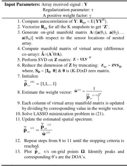
The singular value decomposition based adaptive least absolute shrinkage & selection operator algorithm for underdetermined DOA estimation with reduced dimensionality and complexity is summarized in Table 1.
VI. RESULTS&DISCUSSIONS
In this section, the simulation results for exhibiting the performance of the proposed DOA estimation algorithm: SVD-A-LASSO under various conditions are presented.
The simulation results are based on MATLAB software in conjuction with CVX pacakage for defining and solving convex relaxation problems.
For all the simulations, the regularization parameter τ=2.2 is considered, which optimizes between the sparsity and accuarcy of the solution obtained. A positive weight factor =0.5 is considered for the root-absolute value of solutions obtained previously which are used for weight updations.
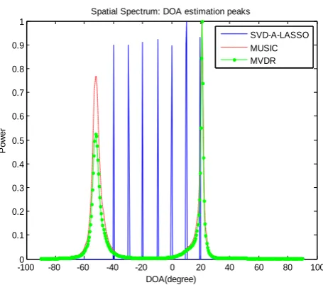
Case-1: In this case, the number of physical array elements taken is M=6, number of signal sources impinging on the array D=2, number of snapshots K=700, SNR=0dB, actual DOA = [-50o, 10o], angular frequencies of the signal sources w= [0.2π, 0.1π] rad/s.
Fig 3 shows the simulation results for case-1, though MVDR and MUSIC algorithms successively indicates the DOA points, they suffer from having less steeper peaks and less non-peak attenuation, whereas the proposed SVD-A-LASSO algorithm exhibits sharp steeper peaks at actual DOAs and negligible non-peak attenuation.
Input Parameters: Array received signal : Y
Regularization parameter: τ
A positive weight factor: 1.1.Compute autocorrelation of Y: Ryy = E{YYH}.
2.Vectorize Ryy for all the K snapshots to get „Z‟.
3.Generate on-grid manifold matrix A=[a(θ1), a(θ2)…. a(θN)] with respect to the sensor locations of nested
array.
4.Compute manifold matrix of virtual array (difference co-array): Ã=(A*A).
5.Perform SVD on Z matrix:
6.Reduce the dimension of Z by truncating: where, SD = [ID 0] & 0 is (K-D)xD zero matrix. 7.Initialize
8.Estimate the weight vector:
9.Each column of virtual array manifold matrix is updated by dividing by corresponding value in the weight vector. 10.Solve LASSO minimization problem in (21).
11.Update the estimated spatial spectrum:
12. Repeat steps from 8 to 11 until the stopping criteria is reached.
13. Plot v/s on-grid points Ω. Identify peaks and corresponding θ‟s are the DOA‟s.
H
ULV
Z (17)
UL
ZV (18)
D D
sv ZVS ULS
Z (19)
} 1
~ ) ( ˆ ~
{ min arg ) (
ˆ 2
2
N
n svn i n i
sv Zsv APsv w p
P (21)
(22)
) 1 ( ) (
~ ˆ
1 ˆ
i sv i
p w
wsv N sv P A sv
Z ~ (20)
} 1 ,... 1 , 1 { ~
ˆ (0)
sv
p
) (
) ( ) (
ˆ ~
ˆ ~
ˆ
i i sv i sv
w p
p
sv
p
~ ˆ
H
ULV Z
D sv ZVS
Z
) 1 ( ) (
~ ˆ
1 ˆ
i sv i
[image:4.595.304.554.80.406.2]p w
TABLE I
[image:4.595.79.291.572.655.2]Case-2: In this case, the number of physical array elements taken is M=6, number of signal sources impinging on the array D=4, number of snapshots K=700, SNR=0dB, actual DOA = [-50o, 0o, 10o, 22.5o], angular frequencies of the signal sources w= [0.2π, 0.1π, 0.3π, 0.4π] rad/s.
Fig 4 shows the simulation results for case-2, as the number of signal sources that are impinging on the array increases more than half the number of physical array elements, MVDR and MUSIC algorithms fails to indicate all the DOA points, whereas the proposed SVD-A-LASSO algorithm clearly indicates all the actual DOA points with sharper peaks.
Case-3: This case shows the effect of highly correlated signal sources on DOA estimation. The number of physical array elements taken is M=6, number of signal sources impinging on the array D=4, number of snapshots K=700, SNR=0dB, actual DOA = [-50o, 0o, 10o, 22.5o], angular frequencies of the signal sources w= [0.2π, 0.2π, 0.2π, 0.1π] rad/s.
Fig 5 shows the simulation results for case-3, MUSIC and MVDR indicates only the signal arriving from 22.5o direction, whereas the highly correlated signals arriving from the directions -50o, 0o, 10o are not detected. The proposed algorithm shows peaks at all the actual DOA points,
indicating that the proposed algorithm also works well in the highly correlated signal source environment.
Case-4: This case shows the simulation results of under-determined DOA estimation. The number of physical array elements taken is M=6, number of signal sources impinging on the array D=7, number of snapshots K=700, SNR=0dB, actual DOA = [-40o, -30o, -20o, -10o, 0o, 10o, 20o], angular frequencies of the signal sources w= [0.2π, 0.3π, 0.4π, 0.5π, 0.6π, 0.7π, 0.8π] rad/s.
Fig 6 clearly indicates that the proposed algorithm can detect all the signal sources even in the situation where the number of signal sources are more than the number of physical array elements (under-determined DOA estimation).
The performance comparison graph of root-mean square error (RMSE) v/s SNR for the proposed algorithm with respect to different values for number of snapshots N is as shown in Fig 7. For lesser number of snapshots, RMSE is high for all the distinct values of SNR considered. The proposed algorithm results in good accuracy if large number of snapshots are measured.
-1000 -80 -60 -40 -20 0 20 40 60 80 100 0.1
0.2 0.3 0.4 0.5 0.6 0.7 0.8 0.9 1
DOA(degree)
P
o
w
e
r
Spatial Spectrum: DOA estimation peaks
[image:5.595.308.535.51.246.2]SVD-A-LASSO MUSIC MVDR
Fig 3. Spatial Spectrum DOA peaks for case-1
-1000 -80 -60 -40 -20 0 20 40 60 80 100 0.1
0.2 0.3 0.4 0.5 0.6 0.7 0.8 0.9 1
DOA(degree)
P
o
w
e
r
Spatial Spectrum: DOA estimation peaks
SVD-A-LASSO MUSIC MVDR
Fig 4. Spatial Spectrum DOA peaks for case-2
-1000 -80 -60 -40 -20 0 20 40 60 80 100 0.1
0.2 0.3 0.4 0.5 0.6 0.7 0.8 0.9 1
DOA(degree)
P
o
w
e
r
Spatial Spectrum: DOA estimation peaks
[image:5.595.45.279.53.246.2]SVD-A-LASSO MUSIC MVDR
Fig 5. Spatial Spectrum DOA peaks for case-3
-1000 -80 -60 -40 -20 0 20 40 60 80 100 0.1
0.2 0.3 0.4 0.5 0.6 0.7 0.8 0.9 1
DOA(degree)
P
o
w
e
r
Spatial Spectrum: DOA estimation peaks
[image:5.595.308.536.275.476.2]SVD-A-LASSO MUSIC MVDR
[image:5.595.46.280.278.476.2]The resolution of the algorithm depends on the step size chosen for defining the grid points. The RMSE decreases with increase in the angle separation between the adjacent signal sources as shown in the Fig 8.
The overall performance comparison of the proposed algorithm with that of the subspace-based algorithm MUSIC and with the CS based framework is presented in Fig 9. It can be observed that the proposed algorithm SVD-A-LASSO has lower RMSE for the lower SNR range from -5dB to +5dB when compared with the other algorithms.
The proposed algorithm later meets the performance level of other algorithms in the higher SNR range.
VII. CONCLUSION
In this paper, an adaptive approach for LASSO minimization for underdetermined DOA estimation with reduced dimensionality by employing singular value decomposition is proposed. The simulation results justify that the proposed algorithm performs better compared to subspace and general CS based DOA estimation techniques in the case where the number of sources to be detected are more than the
number of actual physical array elements. The algorithm also yields good results in the presence of highly correlated sources. The performance of the proposed algorithm with respect to RMSE is considerably good in the low SNR ranges. The overall improvement in the degrees of freedom, complexity reduction, accuracy of the estimation, resolution are the major characteristics of the proposed algorithm.
ACKNOWLEDGMENT
We sincerely thank REVA University, faculty and staff for extending their support in all aspects for the completion of this paper. We also thank our parents and the almighty for all the moral support and encouragement.
REFERENCES
1. R. O. Schmidt, “Multiple emitter location and signal parameter estimation”, IEEE Trans. Antennas Propag, vol. 34, no. 3, pp. 276_280, Mar. 1986.
2. Capon J, “High-resolution Frequency-wave number Spectrum Analysis”, IEEE, Vol. 57, Issue 8, pp 1408-1418, 1969.
3. Richard Roy, Thonas Kailath, “ESPRIT-Estimation of Signal Parameters via Rotational Invariance Techniques”, IEEE Trans on Acoustics Speech and Signal Processing, Vol. 37, No.7, pp 984-995, July 1989.
4. H. Krim and M. Viberg, “Two Decades of Array Signal Processing Research: The Parametric Approach”, IEEE Signal Processing Magazine, vol. 13, no. 4, pp. 67–94, Jul 1996.
5. D. Malioutov, M. Çetin, and A. S.Willsky, “A sparse signal reconstruction perspective for source localization with sensor arrays IEEE Trans. Signal Process., vol. 53, no. 8, pp. 3010_3022, Aug. 2005.
6. Z. M. Liu, Z. T. Huang, and Y. Y. Zhou, “Direction-of-arrival estimation of wideband signals via covariance matrix sparse representation”, IEEE Trans. Signal Process., vol. 59, no. 9, pp. 4256_4270, Sep. 2011.
7. P. Stoica, P. Babu, and J. Li, “SPICE:A sparse covariance-based estimation method for array processing”, IEEE Trans. Signal Process., vol. 59, no. 2, pp. 629_638, Feb. 2011.
8. K. Lee, Y. Bresler, and M. Junge, “Subspace methods for joint sparse recovery”, IEEE Trans. Inf. Theory, vol. 58, no. 6, pp. 3613_3641 Jun. 2012.
9. Z.-M. Liu, Z.-T. Huang, and Y.Y. Zhou, “Sparsity-inducing direction finding for narrowband and wideband signals based on array covariance vectors,'' IEEE Trans. Wireless Commun., vol. 12, no. 8, pp. 1_12, Aug. 2013.
-100 -5 0 5 10 15 20 25
0.5 1 1.5 2 2.5 3 3.5
SNR (dB)
R
M
S
E
(
d
e
g
re
e
s
)
Performance curve: RMSE v/s SNR
[image:6.595.312.545.49.268.2]N=700 N=500 N=100
Fig 7. Performance curve of SVD-A-LASSO: RMSE v/s SNR
1 1.5 2 2.5 3 3.5 4 4.5 5
0 0.05 0.1 0.15 0.2 0.25 0.3 0.35
Adjacent source separation (degrees)
R
M
S
E
(
d
e
g
re
e
s
)
[image:6.595.44.279.52.245.2]Performance curve: RMSE v/s source angle separation
Fig 8. SVD-A-LASSO: RMSE v/s source angle separation
-10 -5 0 5 10 15 20 25
0 1 2 3 4 5 6
SNR (dB)
R
M
S
E
(
d
e
g
re
e
s
)
Performance curve: RMSE v/s SNR
[image:6.595.40.280.301.493.2]SVD-A-LASSO L1-NORM MUSIC
10. J. Yin and T. Chen, “Direction-of-arrival estimation using a sparse representation of array covariance vectors”, IEEE Trans. Signal Process., vol. 59, no. 9, pp. 4489_4493, Sep. 2011.
11. P. Chevalier, L. Albera, A. Férréol, and P. Comon, “On the virtual array concept for higher order array processing'', IEEE Trans. Signal Process., vol. 53, no. 4, pp. 1254_1271, Apr. 2005.
12. W.K. Ma, T.-H. Hsieh, and C.-Y. Chi, ``DOA estimation of quasistationary signals with less sensors than sources and unknown spatial noise covariance: A Khatri_Rao subspace approach,'' IEEE Trans. Signal Process., vol. 58, no. 4, pp. 2168_2180, Apr. 2010. 13. D. Feng, M. Bao, Z. Ye, L. Guan, and X. Li, ``A novel wideband
DOA estimator based on Khatri_Rao subspace approach,'' Signal Process., vol. 91, no. 10, pp. 2415_2419, Oct. 2011.
14. R. T. Hoctor and S. A. Kassam, ``The unifying role of the coarray in aperture synthesis for coherent and incoherent imaging,'' Proc. IEEE, vol. 78, no. 4, pp. 735_752, Apr. 1990.
15. J.-F. Cardoso and E. Moulines, ``Asymptotic performance analysis of direction-finding algorithms based on fourth-order cumulants,'' IEEE Trans. Signal Process., vol. 43, no. 1, pp. 214_224, Jan. 1995. 16. M. B. Hawes and W. Liu, ``Sparse array design for wideband
beamforming with reduced complexity in tapped delay-lines,'' IEEE Trans. Audio, Speech, Language Process., vol. 22, no. 8, pp. 1236_1247, Aug. 2014.
17. M. B. Hawes and W. Liu,, ``Design of fixed beamformers based on vectorsensor arrays,'' Int. J. Antennas Propag., vol. 2015, 2015, Art. no. 181937.
18. P. Pal and P. P. Vaidyanathan, ``Nested arrays: A novel approach to array processing with enhanced degrees of freedom,'' IEEE Trans. Signal Process., vol. 58, no. 8, pp. 4167_4181, Aug. 2010. 19. P. P. Vaidyanathan and P. Pal, ``Sparse sensing with co-prime
samplers and arrays,'' IEEE Trans. Signal Process., vol. 59, no. 2, pp. 573_586, Feb. 2011.
20. K. Han and A. Nehorai, ``Improved source number detection and direction estimation with nested arrays and ULAs using jackknifing,'' IEEE Trans.Signal Process., vol. 61, no. 23, pp. 6118_6128, Nov. 2013.
21. K. Han and A. Nehorai, ``Nested array processing for distributed sources,'' IEEE Signal Process. Lett., vol. 21, no. 9, pp. 1111_1114, Sep. 2014.
22. Y. D. Zhang, M. G. Amin, and B. Himed, ``Sparsity-based DOA estimation using co-prime arrays,'' in Proc. IEEE Int. Conf. Acoust., Speech Signal Process. (ICASSP), Vancouver, BC, Canada, May 2013, pp. 3967_3971.
23. Z. Yang, L. Xie, and C. Zhang, ``Off-grid direction of arrival estimation using sparse Bayesian inference,'' IEEE Trans. Signal Process., vol. 61, no. 1, pp. 38_43, Jan. 2013.
24. R. T. Hoctor and S. A. Kassam, “The unifying role of the coarray in aperture synthesis for coherent and incoherent imaging,” Proc. IEEE, vol. 78, pp. 735–752, Apr. 1990.
25. Pal P, Vaidyanathan P P, “Nested arrays: A novel approach to array processing with enhanced degrees of freedom”, IEEE Trans. Signal Proc. 2010, 58, 4167–4181.
26. Tibshirani, R. Regression shrinkage and selection via the lasso. J. R. Stat. Soc. Ser. B (Methodol.) 1996, 58, 267–288.
27. Zou, H. The adaptive lasso and its oracle properties. J. Am. Stat. Assoc. 2006, 101, 1418–1429.
AUTHORS PROFILE
Raghu K, received master degree in Signal
Processing from VTU, Belagavi, India. He is currently the Ph.D. scholar of the school of Electronics & Communication engineering, REVA University, Bengaluru, India. His research interests include array signal processing, statistical signal processing, sparse representations, direction of arrival estimation etc. He has published 8 international journals. He has been awarded with 1st rank in M Tech Signal Processing by Visveswaraya Technological University, Belagavi, India.
Prameela Kumari N has received her Ph D degree
in Quantum Dot Cellular Automata (Nanoelectronics) from VTU, Belagavi, India. She is currently working as an Associate Professor in the School of Electronics & Communication Engineering, REVA University, Bengaluru, India. Her research interests include VLSI design,