Global optimization: techniques and applications

Rochester Institute of Technology

RIT Scholar Works

Theses

Thesis/Dissertation Collections

5-1-2000

Global optimization: techniques and applications

Nathan Cahill

Follow this and additional works at:

http://scholarworks.rit.edu/theses

This Thesis is brought to you for free and open access by the Thesis/Dissertation Collections at RIT Scholar Works. It has been accepted for inclusion

in Theses by an authorized administrator of RIT Scholar Works. For more information, please contact

[email protected].

Recommended Citation

Global Optimization: Techniques

and

Applications

Nathan

D. Cahill

May

2000

Rochester Institute

of

Technology

Rochester,

NY

14623

Submitted in

partial

fulfillment

of

the

requirements

for

the

degree

of

Master

of

Science in

the

field

of

Industrial

and

Applied Mathematics

Thesis Committee:

Prof. Richard

Orr,

Chair

Dr. Maurino Bautista

Dr. Seshavadhani Kumar

This thesis fulfills the project/thesis requirement

for the degree of Master of Science in the field of

Industrial and Applied Mathematics

at Rochester Institute of Technology

Prof. Richard Orr, Chair

Dr. Maurino Bautista

Dr. Seshavadhani Kumar

RELEASE PERMISSION FORM

Rochester Institute of Technology

Global Optimization: Techniques and Applications

I,

Nathan D. Cahill, hereby grant permission to any individual or organization to reproduce this thesis in

whole or in part for non-commercial and non-profit purposes only.

Abstract

Optimization

problems arise

in

a wide

variety

of scientific

disciplines.

In many

practical

problems,

a global optimum

is

desired,

yet

the

objective

function has

multiple

local

optima.

A

number of

Table

of

Contents

Introduction

3

1

:

Local

Optimization

1.1

Combinatorial Optimization

4

1.2

Continuous Optimization

4

1.2.1 Unconstrained Minimization

5

1.2.2

Constrained

Minimization

9

2: Monte Carlo Global Optimization

2.1 From Local

to

Global Optimization

11

2.2 Random Searches

12

2.3

Simulated

Annealing

13

2.4 Genetic Algorithms

18

3: Deterministic Methods for Global Optimization

3.1 Integer / Mixed Integer

Programming

25

3.2 Unconstrained Optimization: Transformation Methods

27

3.3 Constrained Optimization: Path

Following

31

4: Histogram

Thresholding

for Image Segmentation

4.1 The Image Segmentation Problem

36

4.2

Estimating

Population Mixtures

38

4.3 Simulated

Annealing

for

an

Indeterminate Number

of

Thresholds

40

4.4

Genetic Algorithms for

an

Indeterminate Number

of

Modes

41

5:

3-D Registration

of

Point Sets

5.1 The 3-D Registration Problem

44

5.2 Algorithms for Known Point Correspondence

44

5.3 Global Solutions for Unknown Point

Correspondence

47

Acknowledgments

49

Introduction

Optimization

problems arise

in nearly every

area of science and engineering.

A

chemist

may

want

to

determine

the

minimum

energy

structure of a certain

polymer,

a

biologist may

need

to

investigate

optimal

dosages

and

scheduling

of

drugs

administeredto a cancer

patient,

a civil engineer

may

need

to

decide how many

elevators

to

place

in

an office

building

so

that

waiting

time

is

minimized,

and an

image

scientist

may

wish

to

be

able

to

automatically locate

people

in

an

image.

In

introductory

calculus

classes,

the

most complicated optimization problems students are

faced

with

usually

sound

something

like,

"What

is

the

maximum area

that

can

be

enclosed with a

fence

of

length

Fl"

Even

though theseproblemsteachan

important

lesson,

rarely

can real-world problems

be

solved

solely

by

the

analytical

determination

of points

that

satisfy

first- and second-order

optimality

conditions.

A

typical

optimization problem

takes

the

form:

minimize

fix)

subject

to

x

D

where x ={x\j.z,...jcn)T

is

_{a vector of}

parameters,

and/is

the

objective

function.

In

other

words,

find

x* such

that

^x*)

<

fix)

for

all x e

D.

Note

that

maximization problems can

be

posed

in

this manner

by

negating/.

If D is

a

discrete

set, the

problem

is

referred

to

asa combinatorial optimization problem.

If D is

closed and

/

is

continuous,

this

is

a continuous optimization problem.

This

thesis

will not

focus

on non-smooth optimization problems where

the

objective

function is

discontinuous,

or

non-differentiable,

on a compact set

(for

an analysis of

these

typesof problems see

Chapter 14

of

Fletcher

[15]).

A variety

of methods exist

to

determine local

solutions

(

is

a

local

solution

if

f(\)

<fix)

for

all

x e

N

n

D,

where

N is

a neighborhood of _x')

for both

combinatorial and continuous optimization problems.

For

combinatorial

problems,

a simple choice

is

the

iterative

improvement

method

(a

deterministic

descent

method).

More

sophisticated

methods,

such as the

branch

and

bound

method

(a

method that solves a series of continuous optimization

problems),

are also available.

For

continuous

problems,

a

variety

of

local

minimization methods exist

that

require

function

values

(simplex),

function

valuesand

derivatives (conjugate

gradient and quasi-Newton

methods),

or

function

values,

first

and second

derivatives (Newton

and restricted

step

methods).

If D is

compact,

it

can

be

represented

by

the

intersection

of

equality

and

inequality

constraints.

Such

constrained optimization problems arise

frequently

in

practice and can

be

solved

in

a

variety

of

ways;

many

of which are

based

on

the

idea

of

Lagrange

multipliers.

The

problem of global optimization

is

much more complicated.

Theoretically,

global minimization

is

as simple as

finding

the

minimum of all

local

minima and

boundary

points.

In

application,

this

can

be impractical.

All local

optimization

techniques

require an

initial

feasible

point x(1)

e

D from

which

to

begin

thealgorithm.

In

order to

find

a given

local

minima,

it is necessary

to choose a

feasible

point

that

willconverge to

that minima;

however,

determining

such a

feasible

point can

be

as

difficult

as

solving

the

optimization problem

itself!

Global

optimization can

be

categorized as stochastic or

deterministic.

Stochastic

or

Monte Carlo

methods

(e.g.,

random

search,

Metropolis

algorithm,

simulated

annealing,

genetic

algorithms,

etc.)

randomly

sample

D in

an attempt

to

locate feasible

points

that

are

local

minima

(or

lie sufficiently

close

to

local

minima).

Deterministic

methods

carry

out some non-random search procedure

to

weed through

local

minima and

find

the

global minimum.

For

example,

branching

techniquesset

up

simple sub-problems

to solve,

sub-energy

tunneling

iteratively

transforms the

objective

function

to

remove

local

minima,

and path

following indirectly

locates local

minima

by

solving

a system of

differential

equations.

This

thesis

is broken down into five

chapters.

Chapter 1

gives an overview of

local

optimization methods

for

combinatorial and continuous problems.

Chapters 2

and

3

discuss Monte

Carlo

and

deterministic

techniques

for

global

optimization,

respectively.

Chapters

4

and

5

illustrate

two

difficult

imaging

science problems and

how

they

can

be

attacked with global optimization algorithms.

Chapter

4

discusses

the

thresholding

problem

in image

segmentation,

and

Chapter 5

probes

the

3-D

registration

Chapter 1: Local Optimization

1.1

Combinatorial

Optimization

The

combinatorial optimization problem

has

the

form:

minimize

fix)

(1.1.1)

where x=(xl,x2,...,xn)r

is

_{a vector of parameters.}

We

_can

safely

assume

that

D is

a

finite

set

(if

not,

we can

impose

suitable restrictions on

the

*,-),

and

that

D

is

of sufficient size that a

brute force

search

is

impractical.

Ignoring

multiple

instances

of

the

same

function

value,

we can establish

by

the

Well

Ordering

Principle

that

a global minimum exists.

This

global minimum

is

not

necessarily

unique,

but it

satisfies:

/(x*)</(x)

VxeD

(1.1.2)

In

order

to

attempt

to

solve

(1.1.1),

we

may design

a simple algorithm

that

can

be described in

the

following

steps:

Algorithm (1.1.1): Combinatorial Steepest Descent

(i)

Set

k

=

l.

Choose

_x^.

(ii)

Find

y

such

that

/(y)<

/(x)

for

all xe

Nk

.

(iii)

If

y

=x(k>

,

terminate.

If

not,

set x^+1'=

y

.

(iv)

Set

lc

=

k

+

l.

Goto(ii).

In step

(ii), Nk

is

the

neighborhood of x^

(the

_set

including

x^

and all of

its one-step

transitions).

This

algorithm

is

a steepest

descent

algorithm; that

is,

it iterates

by descending

in

function

value as

fast

as possible.

When

the

algorithm

terminates

at x^,wenotice

that

x^m'

satisfies:

/(x)</(x)

VxeNm

(1.1.3)

Since

x'"1^

does

not

necessarily satisfy

(1.1.2),

it may

not

be

the

global

minimum;

rather

it is

a

local

minimum.

The

steepest

descent

method

described in Algorithm

(1.1.1)

is

a specific

type

of

iterative

improvement

algorithm.

On

each

iteration,

it

selects

the

value

that

most

improves

the

objective

function.

In

general,

iterative improvement

algorithms

only

require

that the

objective

function improves

somewhat on each

iteration.

Such

an algorithm

is

categorized as a

descent

method and can

be

carried out

deterministically

(by

searching

through

the

neighborhood

in

a certain

order)

or

stochastically

(by

randomly

choosing

points

in

the neighborhood)

untilan

improvement is found.

1.2 Continuous Optimization

The

continuous optimization problem

has

the

same

form

as

the

combinatorial optimization problem

in

(1.1.1).

In

this

context

though, D

is

some continuous

domain. If D

is

9T

(or

Cn),

then

(1.1.1)

is

unconstrained.

If D

is

a compact

set,

then

it

can

be

represented as

the

intersection

of a set of

equality

and

inequality

constraints,

and

the

optimizationproblem

takes the

form:

(1.2.1)

minimize

/W

subject

to

c,(x)=0,

ie E

where

E

is

the

set of

equality

constraints and

/

is

the

set of

inequality

constraints.

Analogous

to

(1.1.3),

a point

is

considereda

local

minimum

if

there

exists an e >

0

such

that:

/(x')</(x)

Vxe B(x',e)nZ)

(1.2.2)

where

B(x',e)

is

the

open

ball

of radius e centered at .

If

the

inequality

is

strict,

then we

say

is

a strict

local

minimum.

1.2.1

Unconstrained

Minimization

For

the

standard unconstrained optimization

problem,

we will assume

that

D

=

9T

(nearly

everything in

this

section generalizesto

the

case

D

=

C"

as well).

In

order

to

explain

the

methods used

to

find local

minima,

we must understand

the

properties of

these

minima.

If

is

a

local

minimum of

(

1

.

1

.

1),

then there

are no

descent

directions

at x'.

Mathematically

speaking,

fs(a)=

/(x'+as)

has

zero slope and non-negative curvature at

for any direction

s.

The

zeroslope condition

is

satisfied when

=

0,

where

g

=

V/(x)

is

the

gradient of

/

and

is

given

by:

(1.2.3)

V/(x)=(^/(x)^/(xy.,^/(x)

dx. '

3v

(1.2.4)

The

curvature constraint

is

satisfied when

sTG's>

₀

Vs

*

0

,

where

G

=

V2/(x)

is

the

Hessian

matrix of

/

and

is

given

by:

(1.2.5)

VV(x>

dx2dxi

* ^ '

dx2dx2

^ '

dx2d:

Sr/W ^r/(x)

^-/(x)

dxnd:

dxndx2

(1.2.6)

Conditions

(1.2.3)

and

(1.2.5)

state

that

at

any local

minimum, the

gradient vanishes and

the

Hessian

is

positive semi-definite.

If

the

Hessian is

positive

definite;

i.e.:

sTG s >

0

Vs*0,

(1.2.7)

then the

minimum

is

strict.

Therefore,

(1.2.3)

and

(1.2.5)

are

necessary

conditions

for

a

local

minimum,

and

(1.2.3)

and

(1.2.7)

are sufficient.

(1.2.7)

is

not

easy

to test

in

practice;

any

of

the

following

conditions

are equivalent

to

positive

definiteness

and can

be

easier

to test:

(i)

all eigenvalues of G'

are positive

(ii)

all principal minors of G'

arepositive

(iii)

Cholesky

factors

G' =

LLT

exist with

/,,

positive

Descent

methods with exact

line

search were some of

the

earliest methods

for local

optimization

(Curry

[10]).

These

methods

rely

on

the

fact

that

if

x^

exist a

direction

s^) _such

that

s^ g^_<

₀

.

Then

s^

is

_a

direction along

which

/

can

be

reduced

(a

descent direction).

An

exact

line

search

is

performed

to

locate

the

minimum of

/

along

s^', and the

resulting

point

becomes

next

iterate

x^+1'.

Descent

methods with

line

search can

be described in

the

following

steps:

Algorithm (1.2.1): Descent

methods with

line

search

(i)

Set

Jfc=l.

Choose

x(l).

(ii)

Terminate if

x^

satisfies

(1.2.4)

and

(1.2.5).

(iii)

Choose

s^ _such

that

s^gW

<

0

.

(1.2.8)

(iv)

Find

y>

that

minimizes /(xW+ aH(t)).

(1.2.9)

(v)

Setx(*+1W*)_{+ aHW.}

(vi)

Set

k

=

k

+

l.

Go

to

(ii).

In

general,

it is

not

easy

to

solve

(1.2.9)

exactly;

therefore,

an approximation

to

o>k> _{must suffice.}

A

comprehensive

treatment

of

the

line

search sub-problem

is

given

in Chapter 2

of

Fletcher [15].

At

a

high-level,

an

inexact line

search

is

comprised of a

bracketing

phase,

where an acceptable

interval

of points

is

located,

and a

sectioning

phase,

where

the

bracket is

partitioned

into arbitrarily

small sections until a minimum

is found

to

withina presettolerance.

The

choice of s^

in

(1.2.8)

can

radically

affect

the

convergence properties ofa

descent

method.

An intuitive

choice

is

the

steepest

descent

direction,

the

direction

s^ _that

leads

to the

_{most rapid}

initial

descent in

/

.

The

steepest

direction

at x^

is

that

of

the

negative gradient -g'*'

.

Therefore,

the

steepest

descent

method with

line

search

is

given

by

Algorithm

(1.2.1)

with

(iii)

replaced

by:

(iii)

Set

sW=-gW .

In

practice,

however,

steepest

descent is

a poor method

in

that

it

can exhibit

oscillatory behavior. In

fact,

it

can

be

shown

that

in

certain

instances,

steepest

descent

with exact

line

search appliedtoa simple quadratic

function

does

not

terminate

in

a

finite

number of

iterations!

In light

of

the

poor convergence properties of steepest

descent,

another class of

line

search methods was

developed

thatattempt

to

improve

convergence while

maintaining

some notion of

descent.

These

methods,

called conjugate gradient

methods,

are

based

on the

conjugacy

property

of vectors.

The

vectors s^ _ands'2'

are conjugate with respect

to

G

(or G

-conjugate)

if:

s(l)TGs(2)=

₀

(1.2.10)

For

a simple quadratic

function,

a conjugate gradientmethod can

be

constructed

by

choosing

s^'+1^

to

be

the

component of-g^+1^

conjugate

to

s'^.s'2' s'^

and

performing

a

line

search as

in Algorithm (1.2.1).

The Fletcher-Reeves

conjugategradient method

(Fletcher

and

Reeves

[16])

usesthespecific

formula:

sd)= _g(o,

s(*+o=_g(*+o+I^As(*)

(L2.n)

w

This

method preserves

descent

and

terminates

in

n or

fewer iterations for

a n-dimensional quadratic

function.

Note

that

a positive

definite

quadratic

function

t7(x)

=-LxTGx+ gTx +

b

can

be

minimized

analytically

by

solving

the

system Gx*

=

-g,

but for large-scale

problems conjugate gradient methods

do

Another

family

of

local

minimization methods

is based

on

iteratively

minimizing

quadratic

Taylor

series approximations

to

/

.

Given

a point _x^\

Newton's

method constructs the truncated

Taylor

series

approximation

q^k'(s)

to

/

at x^:

/(x₊s)=

/)()

=

!sTGH

_{+ gWTs +}

/(xW)

(1.2.12)

A

new

iterate

is

computed

by

finding

the

minimum of _c/

(s):

XM)=XW₊

S(*),

(1.2.13)

where gHW=-g^

(1.2.14)

The

system

(1.2.14)

can

be

solved

by

a

variety

of

different

methods.

Solution

by

Cholesky

factorization

enables

the

positive

definiteness

of G^'

to

be

checked.

(1.2.13)

can

be

replaced with a

line

search as

in

steps

(iv)

and

(v)

in Algorithm

(1.2.1)

if desired. If

x'*'

is sufficiently

close

to the

local

minimum x', then

Newton's

methodexhibits second order convergence.

In

general, this

is

much more efficient

than

conjugate gradient

methods,

but Newton's

method

(or

Quasi-Newton

methods)

may be impractical for large-scale

problems.

Newton's

method can also

be

used

in

conjunction with a

line

search carried out

along

s'^ .

The

main

difficulty

with

Newton's

method

is

that the

Hessian

matrix

may only be

positive

definite

in

a small neighborhood of

the

solution.

This

difficulty

can

be

overcome

by

adding

a multiple oftheunit matrixand

solving

the

system:

(*)J.A(*)__(0

(sW

+vI>^

=-gW

(1.2.15)

in

place of

(1.2.14).

This

idea

appeared

originally in

Levenberg

[29]

and

Marquardt [31].

By

selecting

v

so

that

g'^_{+ vI}

is

_positive

definite, (1.2.15)

uses

the

quadratic

information

present

in

(1.2.12)

to

find

the next

iterate

and

eventually

converges

to the

local

solution.

Restricted step

methods

carry

this

modification even

further

by

constraining

thesolution

to

(1.2.15)

to

lie

within some trust

region,

which

is generally

an

ellipsoid or

hyperparallelepiped

centered at x'*^ .

When

second

derivatives

are

difficult (or

inefficient)

to compute,

another

family

of methods

(Quasi-Newton

methods)

can

be

used which approximate the

inverse Hessian

matrix G^*'

by

a positive

definite

matrix H^ and

then

carry

on a

line

search as

in Newton's

method.

The

matrix H^'

is

updated

iteratively

(starting

with some

initial

positive

definite

matrix such as h'1'=

I

)

by incorporating

second

derivative information

obtainedat each

iteration.

In

order

to

do this,

we will

first

expand the gradient

(1.2.4)

about xW:

V/(x(*)₊uW)=

V/(xW)+

^/(x^^^

+

iU^in.

(1.2.16)

This

can

be

rewrittenas:

>)

=g(^i)_gW=G^)+

/p)|n.

(1.2.17)

Therefore,

H^ _can

be

_updatedso

that

h(*+1)v(*)=_u^).

(1.2.18)

A

rank-two

updating

method was proposed

by

Davidon

[12],

Fletcher

and

Powell

[13].

A

rank

H(M=HW+ aiaaT

+ a.2bbT.

(1.2.19)

Since

the

quasi-Newton condition

(1.2.

18)

must

be

satisfied,

we

have

uM=HWvM+aiaaTvM

+ a2bbTvW.

(1.2.20)

If

the

choices a=uSk'

and

b

=H^'V*^ are

made, then

(1.2.20)

reduces

to the

DFP formula:

H^

=

h(*)+^

\

.

(1.2.21)

DFP

U(*)TV(*) v(*FH(*)y(*)

Broyden

[5],

Fletcher

[14],

Goldfarb

[18],

and

Shanno

[41]

introduced

another

updating formula

that

is

the

dual

of

the

DFP formula. The

BFGSformula is

given

by:

Hfc&=H₊

ooth(*)(*)i1i(*v.(*f

1

+

U(*)TVW

L^WV^H^W^l

(*>%(*) u^V*)

(1.2.22)

In

fact,

an

infinite

number of

updating formulas

exist

that

satisfy

the

quasi-Newton condition.

The Broyden

family

of methods

is

given

by

<+1)

=

0H^+(l-*)H^).

(1.2.23)

,(*FV(*)

If

we choose

₀

=

/ ^ , then we

have

a rank one update

to

h'*'.

Both

the

DFP

and ,(*)

U(*)TV(^)_V(^TH(*)V(*)

BFGS

formulae

exhibit

desirable

properties;

they

preserve

the

positive

definiteness

of HK ' _{so a}

descent

direction is

always

chosen,

they

generate conjugate

directions

and

terminate

in

at most n

iterations

for

quadratic

functions,

and

they

exhibit superlinear convergence

for

general

functions.

It

has been

shown

in

the

literature

that

the

BFGS

method

globally

converges when

inexact line

searches are performed

(under

certain

conditions);

consequently,

it has become

the

quasi-Newton method of choice.

When

it becomes difficult (or extremely

inefficient)

to

compute

first

derivatives,

any

of

the

previous methods can

be

used with

finite difference

approximations

to the

gradient vector

(and

the

Hessian

matrix,

for Newton's

method).

Formula

(1.2.24)

shows

how

to

approximate each element of

the

gradient vectorwithcentered

differences:

^/(x+

8ej-/(x-8e,)

(1224)

where

e,

is

the

j'th

column ofthe

identity

matrix.

A

finite difference

approach

is probably

the

best

no-derivative

methods

for

unconstrained

optimization;

however,

it

still

may be

too

costly

to

perform

In

function

evaluations each

iteration.

If

this

is

the case,

other no-derivative methods can

be

used.

The

most popularones are

based

on

the

simplexmethod

(Spendley

et al.

[43]).

In

the

simplex

method,

/

is

evaluatedat a set of

(+l)

equidistant points

in

9T.

A

new simplex

is

formed

by

reflecting

the

point with

the

largest function

valuethrough

the

hyperplane

containing

the

other n points.

When

a point x

has been in

a simplex

for

a given number of

iterations,

the

simplex

is

contracted

by

relocating

the

remaining

n points

half

the

distance

to

x.

Termination generally

occurs when

the

simplex occupies a smaller volume

than

some

threshold.

The Nelder-Mead

method

(Nelder

and

Mead

[34])

is

a simplex method

that

allows

for

irregularly

shaped

simplices,

and

for

expansions as well as contractions

based

on

the

local geometry

of

/

.

In

general, the

simplexmethod can

be

a poor choice

because it does

not guarantee convergence

to

a

local

minimum.

However,

it

can

be very

useful when

attempting

to

optimize

1.2.2

Constrained

Minimization

For

the

standard constrained optimization

problem, the

set

D is

compact and can

be described

by

the

intersection

of

the

equality

and

inequality

constraints of

(1.2.1).

In

unconstrained

minimzation,

any

local

minimum satisfies conditions

(1.2.3)

and

(1.2.5).

In

constrained

minimization,

theseconditions need not

hold.

All

that

is necessary for

a

local

minimum

is

that

no

feasible descent direction

exists.

In

order

to

describe

this mathematically,

let

us

first

consider

the

case where

D

contains no

inequality

constraints

(i.e.,

/

=cj>

). The

following

development is based

on

that

given

in

Chapter

9

of

Fletcher [15].

Suppose

is

a

local

minimizer of

(1.2.1).

Expanding

theconstraints about x',we

have:

+

5)=c,(x')+5Ta;+0|5|).

(1.2.25)

where

a,

=

Vc,(x)

is

the

Ith

column of

the

Jacobian

matrix.

If

we assume

that

8 is

a

feasible

step,

then

c,

(x'

+

5)

=

c,

(x')

=

₀

,so we

know

that

5Ta;=0

V<e.

(1.2.26)

If

the

condition

5Tg'<0

(1.2.27)

holds,

then

8 is

a

descent direction

at .

Since

this

contradictstheassumption

that

is

a

local

minimizer of

(1.2.1),

it

must

be

true

that

no

direction 8

satisfies

(1.2.26)

and

(1.2.27)

simultaneously.

If

we

say

that

g'r^;a;=AV,

(1.2.29)

then we can see that

8Tg'

=

^^5Ta;

_{=0, so}

(1.2.29)

does

not allow

for

(1.2.26)

and

(1.2.27)

to

be

;<=

simultaneously

satisfied

for any 8

.

In

fact,

it

can

be

shown

that

(1.2.29)

must

hold

at a

local

minimum,

so

(1.2.29)

becomes

a

necessary

condition

for

a

local

minimum.

The

condition

(1.2.29)

statesthatat a

local

minimum,

thegradientmust

be

a

linear

combination of

the

constraint gradients.

The

coefficients

(Vs)

f

^e linear

combination are referred

to

as

Lagrange

multipliers.

A

simple

way

to

restate

the

first

order

necessary

conditions arises

from

the

Lagrangian

function:

L(x,X)=/(x)-V;(x).

d-2.30)

i

The

condition

(1.2.29)

is

equivalent

to:

VxL(x'X)=0,

(1.2.31)

and satisfaction of

the

constraints

in

(

1

.2.

1)

is

equivalent

to:

VxL(x'X)=0.

(1.2.32)

<5TV2L(x'Y)8>0

(1.2.33)

for

all

5

*

0 that

satisfy

(1.2.26)

is

a sufficient condition

for

a

local

minimum.

When D

contains

inequality

constraints,

we are

only

concerned with

the

active constraints at a given

minimum; that

is,

the

set of constraints

that

satisfy

c,(x')=0.

We

will

denote

the

active set of constraints at

by

/l'

,and

the

set of active

inequality

constraints at

by

/'

=

rf

c\I.

If

we now observe

the

Taylor

series expansion of

the

constraints at given

by

(1.2.25),

we see that c,(x')=0 and

c,

(x' +

8)

>

₀

, so we

know

that

8Ta;>0

V/e/'.

(1.2.34)

It

can

be

shown

that the

following

conditions must

hold for

(1.2.34)

and

(1.2.26)

to

be

satisfied while

(1.2.27)

is

not satisfied:

=*>;=

AY,

(1.2.35)

X',>0

Vie

I'.

(1.2.36)

Therefore,

any

active

inequality

constraints must

have

positive multipliers.

By

convention,

we

say

that

any

inactive

inequality

constraints correspond

to

zeromultipliers.

The

first-order necessary

conditions

for

minimizationcan

be

restated as

follows:

(1)

vxl(x'X)=q

(ii)

c,(x')=0,

V/e E

(iii)

c,(x')>0,

V/e

/

(iv)

X\

>0,

V/e/

(v)

V;(x')=0,

Vi

These

conditions are

known

as

the

first-order KT

conditions

(Kuhn

and

Tucker [27]).

The

first

two

conditions

follow

directly

from

(1.2.31)

and

(1.2.32). The

third

condition

follows from

(1.2.1),

the

fourth

from

(1.2.36),

andthe

fifth from

the

convention

that

inactive

constraints

have

zero multipliers.

The

theoretical approach

to

solving

constrained minimization problems

is

to

locate

all points

that

satisfy

the

KT

conditions and see

which,

if

any,

satisfy

the

second-order conditions.

This

approach

is

known

as

the

method

of Lagrange

multipliers.

Like

the

theoretical approach

to

unconstrained

minimization,

it is

frequently

difficult,

if

not

impossible,

to

apply

this

method

to

a given "practical" problem.

Because

of

this,

a number of alternate algorithms

have

arisen

based

on

the

structure of

the

objective

function

and constraint

functions.

If

the

objective

function

and constraint

functions

are

linear, (1.2.1)

is

a

linear programming

problem.

A LP

is

most

readily

solved

by

either

the

Dantzig-Wolfe

simplex method

(Dantzig

and

Wolfe

[1

1])

or

the

activeset method.

Both

methods

rely

on

the

fact

that

in

a

LP

problem,

any

extreme value must

take

placeat a vertex of

the

set of constraints.

At

a

high

level,

they

searchthrough

different

vertices of

the

feasible

region,

swapping

constraints

in

andout of

the

active set until a minimum

is

found.

For

quadratic

programming

problems,

where

the

objective

function is

quadratic and

the

constraints are

linear,

a similar activeset approach

is

employed

that

solves

the

equality

constrained

QP

at each

iteration

by

transforming

it

into

an unconstrained

QP (via QR decomposition

or generalized

elimination;

see

Fletcher

[15]).

General

linearly

constrained problems can

be

solved

in

the

same

manner,

by iteratively

transforming

into

an unconstrained

problem,

and

solving

each unconstrained problem

by

a

Quasi-Newton

method,

for

example.

The

most complicated constrained minimization problems are called nonlinear

programming

problems,

Chapter 2: Monte Carlo Global Optimization

2.1 From Local

to

Global Optimization

The

task

of global minimization can

be

daunting

compared

to that

of

local

optimization.

The

theoretical

solution

to the

global optimization problem

is

to

determine

the

set of all points

that

satisfy

(1.1.3)

or

(1.2.2),

sort

them

by increasing

function

value,

and

take the

first

element

(or

elements,

if

the

function

value

is

not

unique)

of

the

set

to

be

the

global minimum.

This

process can

rarely be

carried out

analytically,

unless

the

objective

function

and constraints are simple

in

nature.

In

general,

though,

eventhe

simplest

looking

problems can

be extremely difficult

to

optimize.

It

is

no wonder,

then,

that

many

algorithms

based

on

Monte Carlo

techniques

have

emerged

in

recent years.

One way

to

set

up

a simple

Monte Carlo

algorithm

is

to

represent

the

search space

D

as

the

union of a

finite

number of

(not

necessarily mutually

exclusive)

sets

Sk,

k

=

l,...,N.

In

the

_{case where}

D

is

unbounded,

suitable

lower

and upper

bounds

on

the

parameters must

be

chosen.

A

set of points

jx'^lx^e

Sk,k

=

1,...,n\

is

randomly

chosen,

and each xik)

used as an

initial

point

in

one of

the

local

optimization algorithms

described in

theprevious chapter.

We

will

illustrate

this technique

by

minimizing

the

following

function:

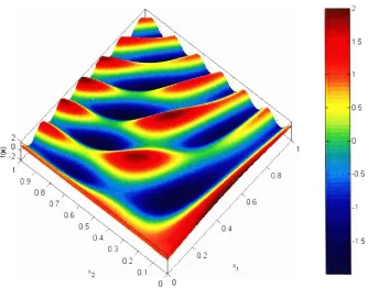
/(x)=

sir^Tu:!

)cos(47tt2)+cos(47t

XyX2)

0

<

xx

<

1,

0

<

x2

<

1

(2.1.1)

As

can

be

seen

in Figure (2.1.

\),

fix)

has many local

minima

in

this

region.

The

globalminimum occurs at

approximately

.

-05

0 o

Figure (2.1.1): Surface

plot of

fix)

We

can

apply

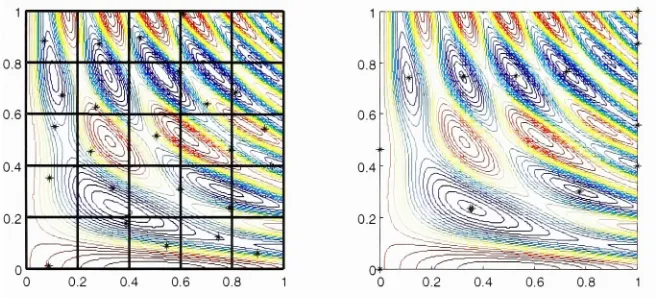
a

Monte Carlo

algorithm

by dividing

the

feasible

region

into

a

5

x

5

grid.

We

then

choose a random point

from

each

patch,

and

apply

the

SQP

method

(Schittowski

[40])

iteratively

with each

random point as a

starting

point.

The left half

of

figure (2. 1

.2)shows

the

5

x

5

grid with a random point [image:15.546.120.454.342.604.2]

chosen

in

each

square,

and

the

right half

shows

the

set of

local

minima

found

by

different

runs of

the

SQP

method.

Note

that

in

this case,

all

local

minima

(including

the

global

minimum)

were

found.

06

%

4*

.;-.

's,...

1.2 0.4 0

Figure (2.1.2): Monte

Carlo

algorithm

for minimizing

fix)

In

order

for

a

Monte

Carlo

algorithm

like

this

one

to

be

robust, the

covering

sets

Sk

should

be

small enough

that

they

can

be

contained within

basins

of attraction of

local

minima.

If

the

Sk

are

too

large,

the

global minimum

may

not

be

found.

On

the other

hand,

if

the

Sk

are

too small, the

algorithm can

become very inefficient. One

major

difficulty

with

this type

of algorithm

is

that

the

only way

to

construct an"optimal"collectionof

covering

sets requires

knowledge

of

the

basins

of attraction ofthe

local

minima.

Another

major problem with

this

Monte

Carlo

algorithm

is

that the

required number of

covering

sets

Sk

increases exponentially

with

the

dimension

of

the

problem.

One way

to

combatthis problem

is

to

keep

track of

the

sets that

have been

visited

during

successive calls

to the

local

optimizer.

If

a

local

optimizer enters a set

that

has previously been

visited, the

local

optimizer can

be prematurely

terminated.

However,

the

Sk

must

be sufficiently

small

(and hence

there

must

be

a

large

number of

them)

in

order

to

reap

the

benefits

ofpremature

termination.

In

some optimization

problems,

it may be very

expensive

to

compute

function

values,

gradient

vectors,

and

Hessian

matrices,

so

performing local

minimizations

from

a succession of points

may be

out of

the

question.

In

these cases, the

only

recourse

(given

current processor

speeds)

is

to

search

for

minima

based

on

function

values alone.

One way

of

doing

this

is

the

simplex

method,

as

described in

Chapter

1.

However,

since

the

simplex method

is

a

local

minimization

method,

global minimization still requires

that

it be

carriedout

from

a

variety

of

initial

points.

More

efficient methods can

be based

on random search

techniques.

The

rest of

this

chapter

discusses

pure and adaptive random

searches,

simulated

annealing,

and

genetic algorithms.

2.2 Random Searches

The

simplest random search technique

is

the

pure random search.

The

algorithm

is very

straightforward:

randomly

generate

N

feasible

points,

and choose

the

point with

the

smallest objective

function

value

for

the

global minimum.

The

pure random search

is

described

as a

descent

method

in

Algorithm (2.2.1).

If

refinement

is

needed,

a

local

minimization can

be

performed

from

the

optimalpoint

found

by

the

search.

The

pure random search

does

not yield an

efficiency improvement

over

the

algorithm

of

Section

2.1;

in

addition,

it

requires

that

N

grow

exponentially

with

the

dimension

of

the

problem

in

order [image:16.546.109.437.143.292.2]

Algorithm (2.2.1): Pure Random Search

(i)

Set

k

=

₀

, c=

0

,

y

= .

(ii)

Randomly

generate x^+1^

e

D

(D

is

the

feasible

region)

(iii)

If

/(x(*+l))<

y

, set

y

=

/(x(*+l))

and

k

=

k

+

1

.

(iv)

Set

c=c+

1

.

If

c <

N

,go

to

(ii).

Patel,

Smith,

and

Zabinsky

[36]

and

Zabinsky

and

Smith

[47]

describe

a pure adaptive search algorithm

that

only

requires

N

to

grow

linearly

with

the

dimension

of

the

problem.

The

PAS

algorithm can

be described

in

the

following

way:

Algorithm (2.2.2):

Pure Adaptive Search

(i)

Set

k

=

₀

,

y

=- .

(ii)

Randomly

generate e

Sk+l

=

{x

I

xe

D

n

/(x)<

>>}.

(iii)

Set

y

=

/(x(,:+l)).

If

k

<

N

,go

to

(ii).

Even

though

this

search method

is

theoretically

more efficient than

the

PRS,

it may be

difficult,

if

not

impossible,

to

generatethenested sets

in step

(ii).

Romeijn

[37]

describes

an adaptive search method

that

differs from

the

PAS

algorithm

in

that

iterates

are chosen

from

the

feasible

region

(i.e.,

Sk

=

D

in step (ii)). The

adaptive nature of

Romeijn's

method

is

that

the

probability distribution

used

to

generate x'A+1'

changes on each

iteration

(not

like

the

PRS,

in

which

the

distribution is generally

uniform).

The

sequence of

distributions is

chosen

to

converge

to the

stationary distribution

of a

Markov Chain. In

the

next

section,

simulated

annealing is

introduced;

this

is

a specific

type

of

Romeijn's

adaptive search method.

2.3 Simulated

Annealing

Since

being

introduced

by

Kirkpatrick, Gelatt,

and

Vecchi

[26]

and

Cerny

[7],

simulated

annealing

has quickly become

one ofthe

best

general purpose

Monte Carlo

global optimization algorithms.

It is

based

on

the

physical modelof

annealing,

where a solid

is

coaxed

into

a minimum

energy

crystalline state

by

slowly

reducing its

temperature.

If

the temperature

is

reducedtoo

quickly,

metastable structures result that

have higher energy

than

the

crystalline state.

The fundamental

building

block

of simulated

annealing

is

the

Metropolis

algorithm,

introduced

some

30

years earlier

by

Metropolis, Rosenbluth, Rosenbluth,

Teller,

and

Teller

[33],

whichsimulates

the

energy

configuration of a

thermally

equilibrating

solid.

This

section will

develop

simulated

annealing in

a combinatorial

setting

andthenshow

how it

can

be

extended

to

thecontinuous case.

When

a solid

is in

thermal equilibrium, the

probability

that the

solid

is

configured

in

a given

energy

state

is

governed

by

the

Boltzmann distribution:

PT(x

=

i)=e-E-/T,

(2.3.1)

where ;

is

a state with

energy

,

(i

can

be

thought of as a vector of parameters and

,

the

corresponding

valueof

the

objective

function),

Z

is

a partition

function,

and

T is

a parameter

that

acts

like

temperature.

When

T

approaches

zero, the

Boltzmann distribution

concentrates

its

mass

in

the

low energy

states.

In

the

limit,

the

only

states with non-zero

probability

are

the

minimum-energy

states.

Metropolis illustrated

that

a combinatorial optimization scheme similar

to

a stochastic

iterative

improvement

algorithmcan

be

constructed so

that the

long-term

probabilities of

the

occurrence of

energy

states approach a

Boltzmann distribution.

The difference between

the

Metropolis

algorithm and a

stochastic

iterative improvement

algorithm

is

that

Metropolis

allows

transitions to

higher-energy

stateswith

positive

probability, whereas,

an

iterative improvement

algorithm

only

allows

transitions to

lower-energy

states.

Because

of

this,

the

Metropolis

algorithm

has

the

potential

to

"jump" out of a

local

minimum

to

explore other

feasible

areas of

the

state space.

The probability

that

a

higher energy

transition

is

accepted

is

given

by:

Pacceptkn

=

; I

x*

=

i.Ej

>,-)=e-{ErEy

.

(2.3.2)

This is known

as

the

Metropolis

criteria.

We

canencapsulate

the

probability

of

accepting

atransition

to

any

state

by:

A(r)=

Paccep,(x,+1

=

j

I xk

=,-)=eHv^>.o}

(2.3.3)

We

can now state

the

Metropolis

algorithm

(note

the

similarities

to

an

iterative improvement

algorithm):

Algorithm

(2.3.1):

Metropolis

algorithm

(i)

Set

k

=

\.

Choose

_x.

(ii)

Randomly

choose x^k+1'

e

Nk

(the

neighborhood of

one-step transitions)

(iii)

Accept

x^'+1'

with

probability

A,y(r).

If

not

accepted,

set x^+1) =x^.

(iv)

Set

k

=

k

+

l.

Go

to

(ii).

No

termination

criteria are

explicitly

stated

in Algorithm (2.3.1).

In

practice, the

algorithm can

be

terminated

whenno substantial

decrease in

function

value

has been

made over

the

last

n

iterations.

It

is

interesting

to

note

that

any

given run of a

Metropolis

algorithm

is

a realization of a

Markov

Chain. In

order

to

constructthe

corresponding probability

transition matrix,

we must not

only

consider

the

transition acceptance probabilities given

by

(2.3.3),

but

the

probability

thata particular state

is

generated

(as in step

(ii)

of

Algorithm

(2.3.1)).

Since

each

iterate is randomly

chosen

from

theset of possible

one-step

transitions

from

the

previous

iterate,

the

generation probabilities are given

by:

Gij

=

Pchoose&k+i

=

J

! x*

=')=

,

rr

(2.3.4)

#ot

states in

Nk

The probability

transition matrix

P(T)

is

found

by

considering both

the

generation and acceptance probabilities:

[

GijAyiT),

j*i

^)

=

l-G,4v(r)

j

=i-

(2-3-5)

[

r*i

Aarts

and van

Laarhoven

[1]

prove

that the

stationary distribution

of

this

Markov

Chain is

indeed

Boltzmann.

Ross

[38]

shows that

the

vectorof

stationary

probabilities

is

a

left

eigenvector of

P(T)

with

corresponding

eigenvalue

X

=

1

.

Therefore,

one

way

to

solve

the

optimization problem

is

to

form

P(T)

and

find

the

appropriate

left

eigenvector.

However,

forming

P(T)

requires

that the

objective

function be

evaluated

for every

possible

state,

which

is

equivalent

to

a

brute force

search.

It

still

behooves

us

to

perform

the

analysis on a small problem.

Consider

a combinatorial optimization problem with

only four

states.

The

possible

transitions

are

indicated

by

arrows

in

the

following

diagram:

o

*_y

o

*^y

o

y^s

o

[image:18.546.163.394.602.646.2]

We

will assign objective

function

values

to

each state:

/(l)

:,=!.

/(2)=2=0,

/(3)=E3=2,

and

/(4)=

4=1.

The

_{generation and acceptance}

probability

matrices can

easily

be

constructed:

G

=

From

(2.3.5),

we can construct

the transition

matrix:

0

1

0

2

0

0

i

0

0

x

2 . A(r)=

0

0

1

0

1

-1/7

1

e "''

1

e

0

1

1

0

0

r^

0

0

2/r

0

1

1

(2.3.6)

p(r)= 2

0

0

1 -2/r

0

-l/r

0

0

2

1-e

(2.3.7)

It

can

be

verified

that

Jt(r)

=

-i/r -i/r

2g"2/r

+

2^

+

2

' e'2'7 + e-1'7 +

1

' e~2lT +

7^

+

1

' 2e"2/r

+2e^T+

2

is

a

left

eigenvector of

p(r)

with unit eigenvalue and

that the

elements of

jt(r)

are

the

masses of a

Boltzmann

distribution.

Also,

it is

clear

that

lim

it(r)=

(0,1,0,0),

so

the

Metropolis

algorithm applied

to this

problem

r->o

can

identify

the

global minimum

if

a

sufficiently large

number of

iterations

are performed and

if T is

small.

One

of

the

most

difficult

aspects of

performing

combinatorial optimization with

the

Metropolis

algorithm

is

the

choice of an appropriate

temperature

parameter.

If T is

too

large,

the

stationary Boltzmann

distribution may

not

be

concentrated enough at the global minimum.

If T is

too

small, the

number of

iterations

required

to

converge

to

the

stationary distribution

can

be

tremendous.

There

is

definitely

a

trade

off

that

must

be

made,

but

the

decision

of

how

to

make

it

can

be very difficult.

Simulated annealing

utilizes a series of

Metropolis

algorithms,

each with smaller

T,

so as

to

converge more

rapidly

to

a

stationary distribution

highly

concentrated at

the

global minimum.

In

terms

ofthephysical

analogy,

a solid

is

cooled

slowly

enough so

that thermal

equilibrium

is

achieved at each

temperature, resulting in

a

minimum

energy

crystalline structure.

Therefore,

much of

the

success of a simulated

annealing

algorithm

depends

on

the

cooling

schedule,

or

the

choice of

decreasing

values of

T.

Simulated annealing

can

be

described

by

Algorithm (2.3.2):

Algorithm (2.3.2):

Simulated annealing

Set

m=

l.

Choose

x(l),

r(l).

Run Algorithm

(2.3.1)

starting

at x(m)

with

T

=T^ .

Set

x'm+1'

to

be

the

state at which

(ii)

was

terminated.

Generate

T^m+1'

according

to

cooling

schedule.

Set

m=_m+

1

.

Go

to

(ii).

(i)

(ii)

(iii)

(iv)

(v)

As

was

the

case

in

the

Metropolis

algorithm, termination

of

step

(ii)

and overall

termination

of

Algorithm

(2.3.2)

can

be

chosen

to

occur

by

a

variety

of means.

For

example, the

user could choose

to

perform a single

iteration

at

step

(ii)

and

have

a

large

number of

slowly-changing

temperatures

in

the

cooling

schedule.

In

this case,

a run ofthealgorithm would

be

a realization of an

inhomogeneous Markov Chain.

For

another

problem,

the

user could choose a

relatively

coarse

cooling

schedule and

terminate

each

Metropolis

algorithm aftera

large

number of

iterations.

Because

the

success and

efficiency

of simulated

annealing greatly

depends

on

the

cooling

schedule,

it

is

important

to

pick a schedule

that

works well.

A

simplegeometric schedule wasproposed

by

Kirkpatrick, Gelatt,

and

Vecchi

[26],

and

many

variantsof

this

method

have

appeared

in

the

literature

since

then.

The initial

value of

T is experimentally determined

so

that the

acceptanceratio

(ratio

ofacceptable

transitions to

possible

transitions

at a given

point)

is

close

to

one

(usually

around

0.95).

Then

the

first

Metropolis

algorithm

is

almost a random walk

through

the

state space.

New

values of

T

are generated

geometrically;

i.e.,

r(m+1)=

aT^m\

witha

typically

between 0.9

and

0.99.

Termination

ofthe algorithm

can occur

if

no substantial

improvement

is

observed over a number of

iterations.

Johnson

et al.

[25]

describe

some other simple

cooling

schedules.

Besides

thegeometric

schedule,

they

describe

a

linear

schedule,

where

T decreases

linearly,

and a

logarithmic

schedule,

where

T decreases

according

to:

rW=

--.,

(2.3.8)

l

+

ln(m)

where

C is

a constant.

They

conclude that none of

these

schedules yield a

dramatic

advantage over

the

geometric schedule.

Aarts

and van

Laarhoven

[1]

describe

a more sophisticated

cooling

schedule.

Like

thegeometric

schedule,

the

initial

valueof

T is

determined

so

that

the

acceptance ratio

is

close

to

one.

New

values of

T

are given

by

the

iteration:

rO+0= jL

8>0,

(2.3.9)

| +

rWln(l

+

5)

3o^>

where

8 is

small and

is

the

standard

deviation

of

function

values

found

during

the

mth

execution of

step

(ii)

of

Algorithm (2.3.2).

If 8 is sufficiently

small,

then

succeeding Markov Chains have

"nearby"

stationary

distributions,

so

the

number of

iterations

required

for

each

Metropolis

algorithm toconverge

is

small.

All

of

the

previous schedules

monotonically decrease

the

temperature.

In

some

instances,

however,

it may be

valuable

to

allow a non-monotonic schedule.

Osman

and

Christofides

[35]

describe

a

"strategic

oscillation"

in

which

T is repeatedly decreased according

to

a geometric

cooling

schedule until

progress

halts,

andthen

increased

to

half

of

its

previous

initial

value.

As

an example of

how

simulated

annealing

can

be

applied to a combinatorial optimization

problem,

let

us considerthe

traveling

salesman problem.

This

problem can

be

stated

in

the

following

way:

a salesman

leaves

home,

visits n

different

houses,

and returns

home.

How

can

the

salesmanconstruct

his

route so

that

the

distance

he

travels

is

minimized?

In

order

to

solve this problem

using

simulated

annealing,

wemust

appropriately define

a state or configuration and a method

for

transitioning

toa

nearby

state.

Each

state can

be

consideredas a possible path

for

the

salesman

to

travel,

and can

be

represented

as a cyclic permutation vector.

For

example,

if

there

are

5

houses,

the state

(13

4 5

2)

represents a path

from house 1

to

house

3

to

house 4

to

house 5

to

house

2

and

back

to

house 1

.

In

general,

for

n

states, there

are

(n-l)!/2

cyclic permutations of

these states,

and

hence (n-l)!/2

possible paths.

Clearly,

there

are

too

many

paths

to

performa

brute

force

search.

We

will

define

a

nearby

state as one

that

can

be

reached

by

a

2-change.

In

a

2-change,

a single element of

the

permutation vector

is

chosen,

and

the

element

directly

to

the

right is

exchanged with

the

element

directly

to

the

left.

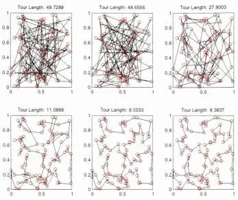
Figure

(2.3.2)

shows

the

results of

applying

simulated

annealing

to the

traveling

salesman problem

with n =

96

randomly

chosen points.

T

was chosen

according

to

a geometric

cooling

schedule witha=

0.98,

and

500 iterations

were performed.

At

each

iteration,

the

Metropolis

algorithm was

iterated

approximately 200

times.

The

plots

in

Figure

(2.3.2)

show samples of

the

initial

path

(upper

left)

and

the

paths afterthe 100th

(upper

middle),

200th

(upper

right),

300th

(lower

left),

400th

(lower

middle),

and500th

(lower

left)

iterations

of a single simulated

annealing

run with an

initial

random path.

Even

though the

solution

is

not

necessarily

the

global minimum

(we

would

have

to

iterate

infinitely

to

guarantee

this),

it

is

a

good solution.

Upon performing

simulated

annealing five

times

for

this

particular

problem,

different

optimalpaths were

found

each

time, but

allof

the

solutions were close

in

total travel

distance

required.

Out

of the

five

trials,

the

best

solution required atravel

distance

of

8.1914

units,

whereas

the

worst required

Tour Length: 49.7289

0.8

0.6

0.4

Tour Length:48,6556

0.8

0.6

0.4

iw|3K

)

0.2,

53t"fii8sm(

>$s55r

Tour Length: 27.8003

0.5 0.5

Tour Length: 11.0868

0.8

0.6

0.4

0.2f

n

TourLength: 8.5533

0.8

0.6

0.4

,

<T\

J

qO ci

0.2{

TourLength: 8.3837

0.5 0.5

Figure

(2.3.2):

Paths

produced

by

simulated

annealing

after

the

0th

(upper

left),

100th

(upper middle),

200th

(upper

right),

300th

(lower

left),

400th

(lower

middle),

and 500th

(lower

right)

iterations.

Simulated annealing

can also

be

applied

to

continuous optimization problems.

In

order

to

extend

the

paradigm

from

combinatorial

problems,

we must

appropriately define

the

generation mechanism and

neighborhood

in step

(ii)

of

Algorithm (2.3.1).

Corana, Marchesi, Martini,

and

Ridella

[9]

describe

an

algorithm where

the

neighborhood

Nk

is

a

hypercube

centered at x^', and a candidate point x't+1'

is

chosen

from

a uniform

distribution

over

Nk

.

If

the

candidate point

is infeasible due

to

equality

or

inequality

constraints,

a new candidate point

is

chosen.

In

order

to

improve

the

efficiency

and convergence properties of

the algorithm,

Corana

etal. update

the

size of

the

hypercube

at each

iteration. If

the

ratioxof

the

number of accepted moves

to the

number of rejected moves

is

large,

the

search

is progressing

too

slowly,

sotheneighborhoodsize should

be increased.

If

this

ratio

is

small,

computational effort

is

being

wasted,

so

the

neighborhoodsize should

be decreased.

Ideally,

x should

be

0.5.

A

suggested scheme

for

updating

the

radius

is

given

by:

r(*+0=

Akh+v

5t-3

,.(*)

1

+

p

2-5t

r(0

T>0.6

T<0.4 ,

otherwise

(2.3.10)

where

(3 is

an

experimentally determined

constant.

The

mechanism

for generating iterates

can also

greatly

influence

the

efficiency

of simulated

annealing.

For

example,

if

a minimum

lies

in

a

long,

narrow

valley,

it is generally

more

fruitful

to

search [image:21.546.103.450.57.349.2]

along

the

axis

through the

valley

than

normal

to

it.

One

way

to

control

the

direction

of search

is

outlined

in

Vanderbilt

and

Louie

[46],

They

describe

a scheme

for generating

steps

according

to

a

probability

distribution

whose covariance matrix

is

proportional

to the

inverse Hessian

matrix.

A

growth

factor

similar

to that

of

Corana

et al.

is

also used

to

control

the

size of

the

search neighborhoods.

We

will

illustrate

the

use of simulated

annealing for

continuous optimization problems

by

minimizing

the

function

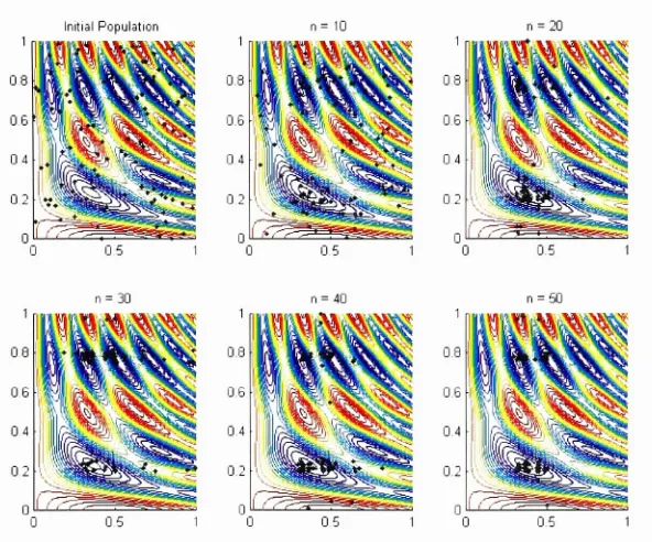
(2.1.1). (We know

that

its

global minimum

is

=

(0.5293,0.7513)T

).

The cooling

schedule used

to

solve

this

problem was

geometric,

with a =

0.98

and

initial

temperature

T

-

10.

Simulated

annealing

was performed at

200

temperature

levels;

at each

level,

100

points were

randomly

chosen and

tested

using

the

Metropolis

criteria.

Figure

(2.3.3)

shows

the

result of one simulated

annealing

run.

The initial

point

is inside

the thick circle,

and

the

best

point

that

was

found (which

is

nearthe true

optimum)

is inside

the thick

square.

All

of

the

other points correspond

to the

best

point

found

at each

temperature

level.

Note

that

simulated

annealing did

a good

job

of

exploring

the

entire

feasible

region

before settling

around a

local

minimum.

In 100

similar

runs, the

solution yielded

by

simulated

annealing

was

in

the

same

basin

of attraction as

the

global minimum

89

times.

0 0.1 0.2 0.3 0.4 0.5 0.6 0.7 0.8 0.9 1

Figure (2.3.3): Simulated annealing

applied

to

Equation (2.1.1). Initial

point

is in

thick circle,

solution

is

in

thick

square.

Other

points are

best

points at each

temperature

level.

There is

one

final

note we need

to

make

in

regards

to

simulated annealing.

Because

of

the

stochastic nature of

this algorithm,

it

can

take

a

huge

number of

iterations

to

yield results of

arbitrary

precision.

Therefore,

it is

recommended

that the

simulated

annealing

solution

is

used as

the

initial

point

in

a

local

optimizer.

This is

a much simpler

way

of

"fine-tuning"

the

result.

2.4

Genetic Algorithms

Genetic

algorithms were

introduced

by

John Holland

[21]

in

order

to

mimic

the

theory

of natural

selection;

that

is,

the

development

over

time

of a species

adapting

to

its

environment.

In

sexual [image:22.546.140.414.224.489.2]

adapt

to

its

environment.

Over

generations, this

dependence

manifests

itself

in

apopulationwhose

level

of adaptation

(or

fitness)

continually improves.

In

order

to

understand

the

basic

genetic

algorithm,

we will

first

introduce

some terminology.

A

population of chromosomes

(or

vectors)

is

changed over

time

by

sexualreproduction.

Each

chromosome

contains a certain number of

traits,

or

genes,

and each gene can

take

on certain

values,

or alleles.

The

fitness

of a chromosome can

be

evaluated

by

assessing its

particular combination of genes.

The

mechanism

of reproduction

is

crossover,

where all

the

genes

up

to

a random position are

taken

from

one

parent,

and all

the

rest of

the

genes are

taken

from

the

other parent.

Occasionally

mutations

take place,

where one or more

alleles are

randomly

perturbed.

The basic

genetic algorithm updates a population of chromosomes

by

sexual reproduction.

Initially,

the

fitness

of

every

chromosome

is

determined;

then,

two

chromosomes are selected

to

reproduce.

Offspring

are produced

by

applying

the

crossover

mechanism; the

offspring may

thenundergo some

degree

of mutation.

Once

the

number of

offspring

produced

is

the same as

the

number of

initial

chromosomes, a

new generation

is formed.

The

new generation

is

treated

as

the

initial

population,

and

the

process

is

repeated until an entire generation exhibits a predetermined

level

of

fitness.

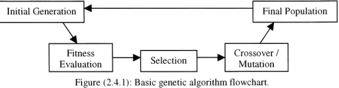
Figure

(2.4.1)

illustrates

the

flow

of a

basic

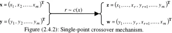
genetic algorithm.

^

Initial Generation

^

Final Population

\

/

Fitness

_h,

Crossover /

Selection

^

Evalu.

ition

w w

Mutation

Figure (2.4.1):

Basic

genetic algorithm

flowchart.

In

the

initial

generation

C

,

there

are n

individual

chromosomes

(typically

anywhere

from 50-200).

Each

chromosome can

be

represented as a vector of

length

m,

where m

is

the

number of genes.

If

x=

(xl,

x2,...,x

is

a

chromosome, then

xt is

the

particular allele of

the

i

gene.

We

will

define

>,

as

theset of possible alleles ofthe

/

gene,

so

that xi

e

>,

.

We

will also

define

D

=

Dx

D2

Dm

as

the

set of all possible chromosomes.

The fitness

of a chromosome x

is

given

by

the

scalar-valued

function

/(x).

In

the selection

step, the

probability

that

a chromosome

is

chosen

is determined

by

its fitness.

Mathematically

speaking,

if

Sj

is

a random variable

representing

the

vector chosen

for

selection, the

distribution

of

S!

is

given

by:

ps,M=

yeC

(2.4.1)

Because

two

chromosomes are selected

for

reproduction,

they

can

be

chosen with replacement

(using

the

distribution

in

(2.4.1))

or without replacement.

If

they

are chosen without

replacement, the

first

vector

chosen

is

SY

,and

the

second

vector,

say

S2

,

has

conditional

distribution:

PSjIS,<