www.hydrol-earth-syst-sci.net/16/873/2012/ doi:10.5194/hess-16-873-2012
© Author(s) 2012. CC Attribution 3.0 License.
Earth System
Sciences
Calibration of the modified Bartlett-Lewis model using global
optimization techniques and alternative objective functions
W. J. Vanhaute1, S. Vandenberghe1, K. Scheerlinck2, B. De Baets2, and N. E. C. Verhoest1
1Laboratory of Hydrology and Water Management, Ghent University, Coupure links 653, 9000 Ghent, Belgium 2Department of Mathematical modelling, Statistics and Bioinformatics, Ghent University, Coupure links 653, 9000 Ghent, Belgium
Correspondence to: W. J. Vanhaute ([email protected])
Received: 17 October 2011 – Published in Hydrol. Earth Syst. Sci. Discuss.: 7 November 2011 Revised: 6 March 2012 – Accepted: 8 March 2012 – Published: 19 March 2012
Abstract. The calibration of stochastic point process rainfall models, such as of the Bartlett-Lewis type, suffers from the presence of multiple local minima which local search algo-rithms usually fail to avoid. To meet this shortcoming, four relatively new global optimization methods are presented and tested for their ability to calibrate the Modified Bartlett-Lewis Model. The list of tested methods consists of: the Downhill Simplex Method, Simplex-Simulated Annealing, Particle Swarm Optimization and Shuffled Complex Evolu-tion. The parameters of these algorithms are first optimized to ensure optimal performance, after which they are used for calibration of the Modified Bartlett-Lewis model. Fur-thermore, this paper addresses the choice of weights in the objective function. Three alternative weighing methods are compared to determine whether or not simulation results (ob-tained after calibration with the best optimization method) are influenced by the choice of weights.
1 Introduction
Rainfall is an important input for many models in various branches of applied sciences. Generally, observed time se-ries of rainfall can be used. However, certain applications (such as design studies) require very long time series which are not available from observations (Wheater et al., 2006). To circumvent this problem, one can make use of rainfall mod-els (Boughton and Droop, 2003). When using such modmod-els, it is of paramount importance to ensure the modelled rain-fall adequately reflects meteorological conditions in the area of interest.
The use of stochastic rainfall models dates back several decades (Waymire and Gupta, 1981), and has since received much attention in literature. Both single-site and spatial-temporal models have been researched extensively. How-ever, the scope of this article is limited to the use of single-site models. For more information about spatial-temporal models, one is referred to Wheater et al. (2005).
An important branch of rainfall models is based on the generation of rectangular pulses. Within these rectangu-lar pulses models, one may discern the Bartlett-Lewis (BL) (Rodriguez-Iturbe et al., 1987a) and Neyman-Scott (NS) (Kavvas and Delleur, 1981) type rainfall models. The dis-tinction between the NS and BL models can be made in the third order moment and proportion dry but not in the second order properties. Hence, both are virtually interchangeable, with the possible exception that the NS models may generate marginally more extreme values. Since empirical analysis revealed that for data observed at Uccle (near Brussels, Bel-gium), the BL model is preferable (Verhoest et al., 1997), and since this paper makes use of the same data (albeit a more ex-tended dataset), the NS models will not be discussed further. Nonetheless, obtained results may also be applicable to the NS models, due to their strong similarity with the BL models. Since the formulation of the original BL model by Rodriguez-Iturbe et al. (1987a), this model has been sub-jected to a number of modifications and extensions. Intro-ducing a jitter, for example, results in more realistically irreg-ular cell intensities (Onof and Wheater, 1994a; Gyasi-Agyei and Willgoose, 1999). Allowing for different cell types to exist, introduces certain variations between storms, which is in accordance with the existence of different types of rainfall
(such as frontal and convective rainfall). To achieve the latter, the mean cell duration can be randomized (Rodriguez-Iturbe et al., 1988), multiple cell types can be defined (Cowpertwait, 1994), or one can make use of multiple superposed processes (Cowpertwait, 2004; Cowpertwait et al., 2007). Finally, to improve extreme value behaviour, the probability distribu-tion of cell intensities can be adjusted to a distribudistribu-tion with a heavier tail (Onof and Wheater, 1994b).
To fit the model to a series of observations, the generalized method of moments is used. In this method, the model is fit-ted to observed sample properties of rainfall intensity at dif-ferent aggregation levels. For this purpose, analytical expres-sions of the expected value of the modelled properties were derived as a function of the model parameters (Rodriguez-Iturbe et al., 1987a).
The calibration of the BL models has proven to be a cum-bersome task because of the presence of multiple local min-ima (Verhoest et al., 1997). Traditional local search tech-niques sometimes fail to avoid these local minima, resulting in a suboptimal solution to the optimization problem.
Furthermore, the calibration result is influenced by the choice of weights in the objective function. Different ap-proaches exist, but it is not clear which of them leads to better simulation results.
To address these issues, this paper proposes to use rela-tively new optimization methods as they are expected to be more robust than more traditional local search methods. Fur-thermore, three different approaches to the weighing of the objective function are compared in order to shed some light on their advantages and disadvantages in terms of model per-formance and practicality. For these purposes, data recorded at the Uccle-site of the Royal Meteorological Institute (RMI) in Brussels (Belgium), are used. The data set consists of 105 yr of recorded rainfall at an aggregation level of 10 min (De Jongh et al., 2006).
2 The modified Bartlett-Lewis model
Aside from the potential adjustments to the original BL mod-elling structure, mentioned in Sect. 1, the basic principles of the model have remained intact: storm arrivals occur in a Poisson process with parameterλ, and each storm arrival is followed by a number of cell origins, which also occur in a Poisson process, characterized by parameterβ. The duration of the interval in which cell origins are generated is expo-nentially distributed with parameterγ. Each cell origin is coupled with a rainfall cell, having a random depth and dura-tion, both drawn from exponential distributions characterized by parameters 1/µx andηrespectively. The superposition
of the rainfall cells eventually leads to a continuous rainfall time series.
Extensive analysis of the model by Rodriguez-Iturbe et al. (1987a,b) revealed that the original BL model was well capa-ble of reproducing general rainfall statistics. Conversely, the
wet-dry properties, commonly expressed by the zero depth probability (ZDP), an important feature of the rainfall time series, were not adequately reproduced. These findings led to an adjustment of the model. In the Modified BL (MBL) model, the average cell duration is allowed to vary between storms. This is achieved by letting the parameter of the expo-nentially distributed cell durationηfollow a Gamma distri-bution with shape and rate parametersαandν, respectively (Rodriguez-Iturbe et al., 1988). This results in E[η] =α/ν and Var[η] =α/ν2. For the expected duration of a cell to be finite, it is assumed thatα >1. Furthermore, Rodriguez-Iturbe et al. (1987a) introduced dimensionless parameters κ=β/ηandφ=γ /η, which are used in the calibration. This way, it can be seen that by keepingκ andφconstant, and varyingη, storms which exhibit similar structures but consist of different types of cells (i.e. with different average dura-tion and variance) are generated. In total, the MBL model contains 6 parameters that are to be calibrated.
Analyses of the MBL model show that the model is an improvement in comparison with the original BL model (Rodriguez-Iturbe et al., 1988; Entekhabi et al., 1989). Bet-ter reproduction of the ZDP, the autocorrelation structure of the rainfall, and the manifestation of extreme rainfall events is observed (Velghe et al., 1994). Nonetheless, the model generates excessive values for the autocorrelation with a lag larger than 12 h (Onof and Wheater, 1993) and the fit of the extremes is still not completely satisfactory.
To improve extreme value behaviour of the model, third order statistics could be included in the objective function. This approach has already proven to lead to good results for the Neyman-Scott models (Cowpertwait, 1998; Burton et al., 2008). Expansion of this concept to the Bartlett-Lewis mod-els can thus be expected to yield similar satisfying results. For the Bartlett-Lewis model at hand, analytical expressions for the third order statistics have not yet been published. However, research on this topic is ongoing and the imple-mentation of third order statistics into the Bartlett-Lewis modelling framework will be addressed in the near future.
3 Calibration procedure
The calibration of Bartlett-Lewis models, and stochastic rain-fall models in general, is usually based on the generalized method of moments (GMM). The GMM seeks to minimize the difference between observed sample properties of rainfall intensity and those generated by rainfall models. Alternative methods, such as likelihood approximation (Cameron et al., 2001) or Bayesian inference (Hartig et al., 2011), could be considered for calibration, but these methods tend to be com-putationally very expensive (Obeysekera et al., 1987). It is not clear whether or not this would have any merit in prac-tical applications (Rodriguez-Iturbe et al., 1988), as from a practical point of view the models are usually treated as be-ing fully identifiable, i.e. only one parameter set is used for
simulation. Moreover, it is not possible to obtain a likelihood function in a closed form, so maximum likelihood approxi-mation is not available as a parameter estiapproxi-mation method.
The use of the GMM for the calibration of stochastic rain-fall models is widespread. An array of empirical studies have been performed in which Bartlett-Lewis models were fitted to rainfall time series in Great Britain (Onof and Wheater, 1993, 1994a; Cameron et al., 2000), Ireland (Khaliq and Cunnane, 1996), Belgium (Verhoest et al., 1997; Vanden-berghe et al., 2011), the United States (Rodriguez-Iturbe et al., 1987b; Velghe et al., 1994), New Zealand (Cowpert-wait et al., 2007), Australia (Gyasi-Agyei and Willgoose, 1999; Heneker et al., 2001), South Africa (Smithers et al., 2002), etc.
In general, the objective function f, which is to be minimized, can be written as:
f (x)=(M0−M(x))TW(M0−M(x)) (1) wherexis the parameter vector,M0is the vector of observed values for a set ofkproperties, M(x)is the vector of their expected values under the model (calculated through analyt-ical expressions), and W is ak×kpositive definite matrix of weights. The objective function valuef for a given set of parametersxis also referred to as the fitness of the proposed parameter vector, as it reflects the quality of this potential solution to the optimization problem.
The chosen fitting properties in the current work include the mean (Avg), variance (Var), lag-1 autocovariance (Cov), and the proportion of dry intervals or zero depth probabil-ity (ZDP). Each of these are evaluated at aggregation levels of 10 min, 1 h, 6 h and 24 h. This is similar to the fitting properties chosen by Cowpertwait et al. (2007).
As discussed in Sect. 1, the parameters of the MBL model all follow a different probability distribution function. The support for each of these parameters is the interval[0,+∞], except forα, for which a lower boundary of 1 is assumed (see Rodriguez-Iturbe et al., 1988). The used algorithms should obey these boundaries, otherwise, numerical instabil-ities might emerge when calculating the analytical expres-sions using negative values, which would trouble the calibra-tion or lead to erroneous results. Another implicacalibra-tion that arises is the impracticality of working with+∞as an upper boundary, as this might impede the convergence of the op-timization method. Therefore, the theoretical upper bound-aries are tightened so that the parameters can still take a wide range of feasible values, and in addition, contain the previ-ously calibrated values of the MBL model (Verhoest et al., 1997). Table 1 shows the set of boundaries which is assumed to constitute the feasible parameter space of the model.
The choice of W is rather subjective. Many different ap-proaches have been explored in literature. The theory of Hansen (1982) suggests that the inverse of the covariance matrix of the observed properties should be used as W. In terms of parameter identifiability, this would be the theoret-ically optimal starting point (Kaczmarska, 2011). However,
Table 1. Pre-defined boundaries for the parameters of the MBL
model during calibration, applicable to all months.
Parameter λ κ φ µx α ν
Lower boundary 0 0 0 0 1 0
Upper boundary 0.1 20 1 15 20 20
for simplicity, in most cases W is chosen to be a diagonal matrix. In that case the objective function is reduced to:
f (x)=
k
X
i=1
wi Mi0−Mi(x) 2
(2)
Frequently,wi is set equal toai/M 0 2
i , whereai is a user
de-fined value (Entekhabi et al., 1989; Cowpertwait, 1991; Vel-ghe et al., 1994; Verhoest et al., 1997; Smithers et al., 2002; Cowpertwait, 2004). Division of the squared model error by the sample estimate ensures that large values do not dominate the minimization procedure (Cowpertwait et al., 2007). The variablea is usually chosen arbitrarily, to ensure a good re-production of certain fitting properties. Cowpertwait (1991), for example, chooses a=100 for the mean and a=1 for the other fitting properties. Velghe et al. (1994) and Ver-hoest et al. (1997), on the other hand, choosea=1 for all fitting properties. In this paper we will follow the approach of Velghe et al. (1994) and Verhoest et al. (1997) and call this objective function OF1.
An alternative configuration of the objective function is suggested by Cowpertwait et al. (2007):
f (x)=
k
X
i=1
" M
i(x) Mi0 −1
2 +
M0
i Mi(x)
−1 2#
(3)
The use of an additional term which contains the reciprocal value of the division present in Eq. (2) helps to ensure that no bias is present in the optimal solution, in case an exact fit is not obtained. This objective function will be referred to as OF2.
Finally, a simplification of the theory of Hansen (1982) can be used to weigh the objective function. Here, wi =1/Var[Mi0] is used. This makes sense because “in
least squares problems with unequal variances, observations should be weighed according to the inverse of their vari-ances” (Chandler, 2004). The empirical variance of the ob-served sample properties is obtained by calculating these properties for each year separately, which results in a series of 105 repetitions of that particular property. The variance of these repetitions is calculated and used in the objective func-tion. This approach will further be referred to as OF3. A more clarifying overview of the used objective functions is given in Table 2.
Finally, it should be mentioned that the MBL model is fit-ted on a monthly basis, i.e. 12 different parameter sets have
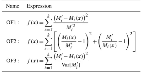
Table 2. Expressions of used objective functions for the calibration
of the Modified Bartlett-Lewis model.
Name Expression
OF1 : f (x)= k X
i=1
Mi0−Mi(x)2
Mi02
OF2 : f (x)= k X
i=1
Mi(x)
Mi0 −1 !2
+ M
0 i
Mi(x) −1
!2
OF3 : f (x)= k X
i=1
Mi0−Mi(x)2 Var[Mi0]
to be calibrated, i.e. one for each month. This approach is upheld to cancel out any seasonal effects present in the rainfall time series. This is necessary to ensure temporal homogeneity (Obeysekera et al., 1987; Verhoest et al., 1997). The objective of this paper is to determine whether the choice of the objective function has a significant impact on the estimated parameters. If this is the case, the impact of the choice of the objective function can be assessed by consid-ering properties that were not used during the fitting, but are of hydrological importance. If no significant impact can be observed, a distinction can be made based on the efficiency of the calibration.
4 Optimization methods
The calibration of the Bartlett-Lewis models has been re-ported as being a cumbersome task (Verhoest et al., 1997), as the optimization is troubled by the presence of multiple local minima, in which local optimization techniques tend to get trapped. In the past, such techniques have been used in the majority of the cases. For example, Velghe et al. (1994); Verhoest et al. (1997); Onof and Wheater (1993) use Powell’s method (Press et al., 1986) for calibration. This gradient-based method is prone to get stuck in local optima. Fur-thermore, the user has to supply the algorithm with an initial guess of the solution, which may lead to a bias in the results (Khaliq and Cunnane, 1996). More recently, most authors opt to calibrate using the Simplex method by Nelder and Mead (1965) with multiple starting points. Occasionally the outcome is further minimized using a gradient-based method (Wheater et al., 2006; Cowpertwait et al., 2007; Kaczmarska, 2011).
In recent years, an array of global optimization methods has been developed. In this work, we test four of those algo-rithms with respect to the calibration of the BL models. The following sections discuss the theoretical background of the used optimization methods which, ultimately, stem from fun-damentally different conceptual backgrounds. The current paper does not aim at discriminating against or rallying for a certain method, merely an objective comparison,
highlight-ing advantages and disadvantages of the presented methods is aspired.
4.1 Downhill simplex method
The Downhill Simplex Method (DSM) is based on an idea by Spendley et al. (1962) for tracking ideal operating conditions by evaluating the output of a system at a set of points, form-ing a simplex, in the parameter space, and the continuous formation of new simplices by reflecting a point in the hyper-space of the other points. Nelder and Mead (1965) acknowl-edged this concept’s merit in the optimization of mathemat-ical formulas. The simplex moves autonomously through the parameter space by a sequence of intermittent reflections, contractions and expansions.
Suppose an objective function containsD variables and is subjected to a minimization procedure without posing any restrictions on the values of the variables. Then, suppose
x0,x1, . . . ,xDare (D+1) points in theD-dimensional space
which form the current simplex. The objective function value of each pointxiis written asyi.
The point with the lowest objective function value receives the subscriptl(yl=min
i yi), the point with the highest
objec-tive function value receives subscripth(yh=max
i yi). Point
¯
xis defined as the centroid of those points for whichi6=h. The distance betweenxi andxj is expressed by d(xi,xj).
During each step of the process,xhis replaced by a new point
by a reflection, contraction or expansion of the simplex. The reflection ofxhcan be written asx∗h, whose coordinates can
be found by the following relationship :
x∗=(1+α)x¯−αxh (4)
withαa positive constant, known as the reflection coefficient. In other words,x∗lies on a straight line, connectingxhand
¯
x, opposite tox¯, with d(x∗,x¯) = αd(xh,x¯). xh is replaced
by x∗h and the process starts over with the new simplex if yh> y∗> yl.
If, on the other hand, the reflection has created a new min-imum (y∗< yl), the simplex is expanded fromx∗ towards
x∗∗according to :
x∗∗=γx∗+(1−γ )x¯ (5)
The expansion coefficientγ, which is larger than 1, equals d(x∗∗,x¯) divided by d(x∗,x¯). Ify∗∗< y
l, thenxhis replaced
by x∗∗ and the process starts over. If, on the other hand, y∗∗> yl, then the expansion is considered to have failed and
xhis replaced byx∗before re-initiating the process.
If the reflection of x to x∗ results in a situation where y∗> yi for all i6=h, i.e. replacing x by x∗ results in the
creation of a new maximumy∗, thenxh becomes eitherxh
orx∗, whichever has the smallest function value, andx∗∗is calculated as follows :
x∗∗=βxh+(1−β)x¯. (6)
The contraction coefficientβ∈[0,1] is the ratio of d(x∗∗,x¯) to d(x,x¯). x∗∗ replacesx
h and the algorithm proceeds to
the next iteration, unlessy∗∗>min(yh,y∗). In the latter case
the contraction resulted in a point that has a higher function value than bothxhandx∗. In case of such a failed
contrac-tion allxi’s are replaced by(xi+xl)/2 before continuing to
the next iteration. The propagation of the simplex continues until a suitable result (expressed by the stopping criteria) is obtained.
As can be deduced from the description above, the DSM is a local, rather than a global search method. The outcome of the optimization strongly depends on the initial position, provided by the user. To enable a more global search, and to avoid a biased outcome resulting from a user provided initial position, multiple starting points are chosen randomly within the boundaries of the search space. In this specific case 30 initial positions are generated. The DSM is applied to each of these initial positions, after which the single best result is selected as the outcome of the DSM with multiple starting points. This method is used throughout the article, any fur-ther mentioning of the DSM thus refers to the methodology using 30 initial positions.
4.2 Simplex-simulated annealing
Simplex-Simulated Annealing (SIMPSA) is a hybridization between the DSM by Nelder and Mead (1965) and Simu-lated Annealing (Kirkpatrick et al., 1983; Kirkpatrick, 1984). The latter method, which is based on the metallurgic pro-cess of Annealing, enforces the DSM through its abil-ity to escape local minima and thus avoid premature con-vergence. The annealing process was first simulated by Metropolis et al. (1953), and was later picked up by Kirk-patrick et al. (1983), to be used as an optimization algorithm. In the original Metropolis algorithm, an equilibrium com-position of molecules, which yields minimum energy at a given temperature, is sought after through successive ran-dom displacements. Because a thermic balance is charac-terized by a Boltzmann distribution of energy levels, tran-sitions towards a lower, as well as towards a higher en-ergy level are possible. This feature is thought to be the main reason why a minimum energy level can be reached (Aarts and Van Laarhoven, 1987).
This concept can easily be translated towards an optimiza-tion algorithm. By replacing the energy level of the system with the value of an objective function, the search for a min-imum energy level is converted to a search for the minmin-imum of the objective function. As stated before, this leads to an optimization scheme which is fairly consistent and, above all, less prone to get stuck in local minima, in comparison with gradient-based methods. An issue, however, is that Simu-lated Annealing relies on a random walk through the param-eter space. This shortcoming can be mitigated by the use of the DSM to guide the search of the optimum, which al-lows for a more structured search. This is what constitutes
SIMPSA (Press and Teukolsky, 1991; Cardoso et al., 1996). From the point of view of the DSM, the incorporation of the Simulated annealing framework enforces the DSM in its global search. By allowing occasional missteps, the algo-rithm can be steered away from local minima, increasing the robustness of the outcome.
The probability of a misstep is controlled by the temper-ature T of the system. A new configuration correspond-ing to a lower energy level (i.e. 1E <0) or lower func-tion value, is uncondifunc-tionally accepted. When, on the other hand, a solution is found which cannot be accepted as an im-provement (i.e. 1E≥0), there still is a chance P (1E)= exp(−1E/ kbT )that it will nevertheless be accepted. Thus, the probability of making a move in the “wrong” direction is very high at the beginning of the cooling process, i.e. a global search of the parameter space in conducted. As the temper-ature decreases, the chances of making a wrong move de-crease accordingly, approaching zero and thus the algorithm ultimately converges towards the original DSM.
It is clear that, in order to fully exploit the potential of SIMPSA, the initial temperature has to be chosen carefully, satisfying the condition that almost all wrong steps should be accepted at the start of the iteration process. Then, as the optimization progresses, the chances of making erroneous moves should decrease, which means the temperature will steadily decrease according to a predefined cooling schedule. The cooling schedule proposed by Aarts and Van Laarhoven (1985) is used :
Tj+1= T
j
1+Tj·ln(1+δ) 3σ
(7)
withδ andσ trajectory parameters, and j the current iter-ation. δ is the cooling rate, which controls the speed of the cooling. Small values (<1) will result in slow conver-gence while larger values (>1) result in convergence to in-ferior local minima. Finally,σ is the standard deviation of the objective function value of all configurations at a certain temperatureTj at iteration stepj.
In order to initiate the optimization scheme an initial guess of the parameter vector has to be supplied by the user. This initial guess is used by SIMPSA to construct the additional D points of the simplex needed in a D-dimensional prob-lem. Therefore, the initial guess is perturbed in one of itsD dimensions to create the initial simplex. Once the initial sim-plex is formed, the iteration process can commence and new simplex configurations are formed like in the original DSM. The way in which SIMPSA incorporates the Simulated Annealing methodology of making the occasional faulty move is as follows: when propagating the simplex follow-ing the aforementioned rules (Sect. 4.1), a positive, log-distributed variable, proportional to the control temperature T, is added to the function value of each of the points of the simplex. In a similar fashion, the function value of the newly found point is diminished by a randomly chosen value. In
this manner, a new point (e.g. created by a reflection) with a higher objective function value than the other points of the simplex (which would be rejected by the DSM’s rules), still has a chance (proportional toT) of being accepted.
4.3 Particle swarm optimization
The accomplishment of complex objectives through the use of simple individual interactions has been an important source of influence for a certain type of artificial intelli-gence, collectively termed Swarm Intelligence. One of those techniques is Particle Swarm Optimization (PSO), initially introduced to simulate social behaviour and later adapted to be used as an optimization method (Kennedy and Eber-hart, 1995). PSO is based on the behaviour of herd ani-mals, characterized by the absence of a leader in the herd. Notwithstanding the absence of such a leader, the herd is able to act as a collective, mainly due to local interactions between the individuals. This allows them to attain certain goals, such as the gathering of food and the evasion of preda-tors. The simulation of this behaviour and the replacement of the aspired goal by some sort of objective function, makes this method particularly useful for solving an optimization problem (Engelbrecht, 2006).
The PSO algorithm consists of a swarm ofN particles, each particle representing a possible solution to the problem at hand. The particles travel the multi-dimensional search space, in search of the global optimum. The search is led by a combination of information gathered by the particle it-self, and by the community as a whole. In aD-dimensional search space, the position and velocity of a certain particle i, withi=1,...,N, can be represented by aD-dimensional vectorxi=(xi1,xi2,...,xiD)andvi=(vi1,vi2,...,viD),
re-spectively. The positionxi of a particle can be adjusted by
adding its speed vectorvi to the current position. This can
be expressed by the following equation:
xi(t+1)=xi(t )+vi(t+1) (8) for which t and t+1 express the current and subsequent iteration step.
The velocity drives the optimization. It determines the speed and direction in which the particles move, thus orches-trating the collective search of, and convergence towards, the global optimum. For this purpose, the aforementioned vector is equipped with two components, each containing specific information about the objective. (1) The cognitive
component reflects the personal experience of a given
parti-cle, while (2) the social component bears information gath-ered by the particle’s neighbourhood. Many different ap-proaches exist for defining the size and shape of this neigh-bourhood, more detailed information can be found in Engel-brecht (2006). For the sake of simplicity, a global neighbour-hood is selected for the current application. The social com-ponent thus consists of information gathered by the swarm as
a whole during all preceding iterations and the current, and is represented by the best found positionpgby the swarm. Ac-cordingly, the cognitive component consists of information about the objective function, obtained by a certain particlei. It is expressed by the best previously visited positionpi of
particleiin the search space. Both components are combined to update the velocity:
vi(t+1)=w·vi(t )+c1·r1(t )· [pi(t )−xi(t )]
+c2·r2(t )· [pg(t )−xi(t )], (9)
withvi(t )the velocity of particleiat iteration stept;xi(t )
the position of thei-th particle at iteration stept;c1andc2 positive acceleration constants, used to scale the influence of the cognitive and social components. The variablesr1(t ) andr2(t )are uniformly distributed between 0 and 1, and in-troduce a stochastic component in the optimization. Finally, w is the inertia weight. These parameters all have an im-portant influence on the performance of the PSO algorithm, a more detailed discussion of their significance and a method for their selection are reported in Sect. 5.2.
4.4 Shuffled complex evolution
The Shuffled Complex Evolution algorithm (SCE-UA), orig-inally developed for the calibration of a watershed model (Duan et al., 1994), is based on a synthesis of four con-cepts: (1) a combination of deterministic and probabilis-tic approaches; (2) systemaprobabilis-tic evolution of a “complex” of points spanning the parameter space, in the direction of global improvement; (3) competitive evolution; (4) complex shuffling. The combination of these concepts, most of which have already proven their merit in global optimization prob-lems, makes the SCE-UA method robust, effective, flexi-ble and efficient (Duan et al., 1994). The SCE-UA method (following the description by Duan et al., 1994) can be summarized by the following steps:
1. at the start of the optimization procedure a random sam-ple ofs points is generated in the feasible parameter space (defined by the user). Since no prior information about the approximate location of the global optimum is available, a uniform distribution is used to generate this initial sample. In each of thespoints, one can calculate the corresponding objective function value.
2. Once the objective function values of the generated samples are known, they can be ranked according to their objective function values, the first having the low-est function value and the last having the highlow-est func-tion value (or the other way around for a maximizafunc-tion problem).
3. Thespoints are then partitioned intopcomplexes, each containing m points. The complexes are partitioned in such a manner that complexi, where i=1,2,...,p,
contains every p(k−1)+i ranked point, with k= 1,2,...,m.
4. The constructed complexes are allowed to evolve ac-cording to the competitive complex evolution (CCE) al-gorithm (which will be discussed further below). 5. After the complexes have evolved they are shuffled.
This is accomplished by combining them into a single sample population: sorting the population in order of increasing objective function value and ultimately shuf-fling the sample population intopcomplexes following the procedure outlined in step 3.
6. Before continuing the iterative process convergence cri-teria are checked. If none of them are met the pro-cess continues, otherwise the propro-cess is aborted and the optimum is assumed to have been found.
7. In a final step the reduction of the number of complexes is checked. If the minimum number of complexes re-quired in the population,pmin, is less thanp, then the
complex with the lowest ranked points is removed,pis replaced byp−1 ands=pm, after which the process restarts at step 4. If, however,pmin=p, the algorithm
returns to step 4.
The effectiveness of the SCE-UA method can be attributed to several factors. First of all the use of a population avoids biases resulting from the use of a single user-defined initial point. On the other hand, the partitioning into different com-plexes allows for an extensive exploitation of the parameter space, while the shuffling of the complexes is a way of shar-ing knowledge on a larger scale, representshar-ing the explorative character of the algorithm.
A key component of the SCE-UA method is the CCE al-gorithm. The CCE algorithm controls the evolution of the points within a certain complex. Within each complex, a sub-complex is formed. A fixed number of points is drawn from a trapezoidal probability distribution (constructed so that the point with the best function value has the best odds of being selected) and are assigned to the subcomplex. The mem-bers of the subcomplex can be regarded as parents which are about to generate offspring. The idea of competitive-ness, introduced in the formation of the subcomplexes (not all points of the complex are allowed to procreate), expedites the search towards promising regions. Offspring is generated via the use of the DSM by Nelder and Mead (1965). The simplex is formed by the points of the subcomplex, and is allowed to progress for a fixed number of inner loop itera-tions (nI), resulting in the offspring. The generation of off-spring is repeated a number of times before the complexes are shuffled and the process starts over. As the optimization progresses, the entire population is expected to converge to-wards the neighbourhood of the global optimum, provided that the initial population size and the number of complexes is sufficiently large.
5 Implementation of the optimization methods
For each of the optimization algorithms described, several parameters have to be selected in order to fully exploit their potential. The selection of those parameters will have an influence on the effectiveness of the algorithms, so a care-ful consideration of the available options will contribute to the objectiveness of the overall comparison. Therefore, the conducted selection procedure for the parameters of the op-timization algorithms is described below. Furthermore, the implementation entails the specification of measures to be taken against infeasible parameter combinations, i.e. points which lie outside the delineated boundaries. These measures will also be described in the following sections.
All algorithms that are based on a simplex design are stopped by the same stopping criteria. The iterative process is called to a halt when the differences in objective func-tion values between the points of the simplex are smaller than a certain threshold, or when the positions of the simplex points differ less than a given threshold. For PSO, other cri-teria need to be specified because of the different conceptual approach. This is further elaborated in Sect. 5.2.
5.1 Simplex-simulated annealing
The performance of SIMPSA can be enhanced for a specific problem by fine-tuning some of the parameters of the algo-rithm. Most of the parameters have been set to their recom-mended value (Cardoso et al., 1996), except for the cooling rateδ (see Eq. 7) and the final temperature. To avoid the al-gorithm getting stuck in local optima, it is opted to choose the cooling rateδ <1, which will lead to slower but steady convergence instead of fast convergence towards (possibly) inferior optima. Therefore, different cooling rates are tested, δis varied between 0.2 and 0.9 with an increment of 0.1.
The second parameter that can be adjusted is the final tem-perature. The final temperature is the temperature at which SIMPSA is reduced to the original DSM. Put differently, if the final temperature is reached, the temperature is set to zero and the chances of making movements in the wrong direction become equal to zero. Obviously, the higher the final temper-ature, the faster the algorithm will come to a halt. Care must be taken however, a final temperature that is too high will nullify the expected advantages of using SIMPSA instead of the DSM. Different values for the final temperature are tested to investigate its influence on the overall calibration result. The final temperature is tested at{1, 0.1, 0.01, 0.001, 0.0001, 0.00001}.
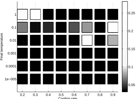
Figure 1 shows the dependence of the objective function value on the cooling rate and the final temperature. For each month, calibrations were performed using these differ-ent combinations for cooling rate and final temperature. Fig-ure 1 displays the average result obtained over the different months, so as to provide an image on how well the combi-nation of cooling rate and final temperature performs for the
880 W. J. Vanhaute et al.: Calibration of the modified Bartlett-Lewis model
0.2 0.3 0.4 0.5 0.6 0.7 0.8 0.9
1
0.1
0.01
0.001
0.0001
1e−005
Cooling rate
Final temperature
0.05 0.1 0.15 0.2 0.25
Fig. 1: Dependence of the fitness on the cooling rate
δ
and
the final temperature of SIMPSA
0.5 0.7 0.9 1.1 1.3 1.5 1.7 1.9 2.1 2.3 2.5
0.5
0.7
0.9
1.1
1.3
1.5
1.7
1.9
2.1
2.3
2.5
c
2
w = 0.4
c
10.5
1
1.5
2
2.5
(a)
0.2 0.4 0.6 0.8 1
0.5
0.7
0.9
1.1
1.3
1.5
1.7
1.9
2.1
2.3
2.5
w
c
2
= 2.5
c
11
2
3
4
5
6
7
8
(b)
0.2 0.4 0.6 0.8 1
0.5
0.7
0.9
1.1
1.3
1.5
1.7
1.9
2.1
2.3
2.5
w
c
1
= 1.5
c
21
2
3
4
5
6
7
8
(c)
Fig. 2: Dependence of the objective function value on the
different parameters of PSO
Fig. 1. Dependence of the fitness on the cooling rateδand the final temperature of SIMPSA.
calibration of all months. It should be noted that for different combinations of cooling rate and final temperature, the same minima are obtained. To highlight this, and to increase inter-pretability of the plots, the color scale of Fig. 1 (and of plots in the following sections) is adjusted so that only parame-ter combinations with the lowest obtained objective function values are attributed gray shades. Parameter combinations that resulted in the minima are attributed a black colour.
Results confirm that for lower final temperatures better re-sults are obtained, this is because the parameter space is ex-plored more intensively. For the cooling rateδ, it seems that the best results are obtained when it is set to 0.5 or 0.8. Fig-ure 1 shows that forδ=0.5 andδ=0.8 equally good results are obtained for different final temperatures. We choose to setδequal to 0.5, to favour a slower convergence, minimiz-ing the risk of gettminimiz-ing stuck in a local optimum. The final temperature is set to 1, as this will lead to a faster calibration than would be the case if the final temperature were to be set lower.
Besides the choice of the above-mentioned parameters, the user has to set up rules about what to do with generated points which are outside the parameter boundaries. One possible way is to just place boundary violating points at the bound-ary (Box, 1965). This, however, may lead to considerable instabilities in the simplex which may cause it to collapse (Cardoso et al., 1996). Another solution is to reset them at a random position in the feasible parameter space. In this paper, we opted for accepting infeasible points, however, the objective function is adjusted so that infeasible points auto-matically receive a very high objective function value, which will force the simplex back into the feasible parameter space (Nelder and Mead, 1965). Note that the same approach is used for the DSM.
5.2 Particle swarm optimization
As outlined in Sect. 4.3, the performance of PSO is influ-enced by several parameters. To ensure efficient convergence to the global optimum, care must be taken in the selection of these parameters. For example, the population sizeN must be chosen large enough so that the parameter space is suf-ficiently explored, but not too large because of the obvious increase in computational burden accompanied with such an increase in population size. Furthermore, the cognitive pa-rameterc1, social parameterc2and the inertia weightwwill also have an impact on the speed and efficiency of the al-gorithm. The relative magnitude ofc1andc2determine the exploration/exploitation trade-off made by PSO. Exploration means the particles will be able to explore the whole param-eter space and identify promising paramparam-eter regions. They will, however, lack in accuracy to find a satisfactory optimum in this promising region. Exploitation, on the other hand, means each particle will be pre-occupied with its own local search, not interacting much with the other particles. This way, the parameter space will not be explored sufficiently, so inferior results might be obtained. For the PSO algorithm to work properly, the balance of the exploration/exploitation trade-off is of key importance. A larger social parameter c2, for example, means that more importance is given to the global best position, i.e. exploration is favoured. If, on the other hand, the cognitive parameterc1 outweighs the social parameter, much more care is given to the local exploita-tive search by the particles. Finally, the inertia weight w (0< w <1)will slow down the velocity of the particle at a previous iteration step. Large values ofwfacilitate explo-ration of the parameter space (higher velocities will lead to more extensive coverage of the parameter space), whilst a smallwfacilitates exploitation (Engelbrecht, 2006).
To select the parameters which will lead to the best cali-bration results for the model under study, an exhaustive pa-rameter search is conducted (Scheerlinck et al., 2009). Pa-rameters c1, c2 and w are varied and monthly calibrations are conducted for the different combinations. The population sizeNis fixed at 30 particles (Engelbrecht, 2006). The other parameters are varied in their convergence domain (Trelea, 2003; Jiang et al., 2007). Parametersc1andc2range from 0.5 to 2.5 andwranges from 0.2 to 1 with an increment of 0.2.
Figure 2 displays the results of the exhaustive parameter search. This figure shows the mean obtained objective func-tion value for the monthly calibrafunc-tions. For the three param-eters, a value can be chosen such that, on average, the al-gorithm performs well for all months. Figure 2a shows the dependence of the fitness with regard to the social and the cognitive parameters,c1andc2, with a fixed inertia weight (w=0.4). The results show that, in order to obtain good cal-ibration results, a trade-off has to be made betweenc1andc2. High values ofc1in combination with low values ofc2yield good results and vice versa. A choice thus has to be made by the user in favour of either a more explorative, or a more
[image:8.595.50.286.62.234.2]W. J. Vanhaute et al.: Calibration of the modified Bartlett-Lewis model 881
16 W. J. Vanhaute et al.: Calibration of the modified Bartlett-Lewis model
0.2 0.3 0.4 0.5 0.6 0.7 0.8 0.9 1 0.1 0.01 0.001 0.0001 1e−005 Cooling rate Final temperature 0.05 0.1 0.15 0.2 0.25
Fig. 1: Dependence of the fitness on the cooling rateδand the final temperature of SIMPSA
0.5 0.7 0.9 1.1 1.3 1.5 1.7 1.9 2.1 2.3 2.5 0.5 0.7 0.9 1.1 1.3 1.5 1.7 1.9 2.1 2.3 2.5 c 2
w = 0.4
c1 0.5 1 1.5 2 2.5 (a)
0.2 0.4 0.6 0.8 1 0.5 0.7 0.9 1.1 1.3 1.5 1.7 1.9 2.1 2.3 2.5 w c
2 = 2.5
c1 1 2 3 4 5 6 7 8 (b)
0.2 0.4 0.6 0.8 1 0.5 0.7 0.9 1.1 1.3 1.5 1.7 1.9 2.1 2.3 2.5 w c
1 = 1.5
c2 1 2 3 4 5 6 7 8 (c)
Fig. 2: Dependence of the objective function value on the different parameters of PSO
Fig. 2. Dependence of the objective function value on the number of
complexespand the number of inner loop iterationsnIof SCE-UA.
2
5
10
15
10
20
30
40
50
100
Number of complexes
Number of inner loop iterations
0.2
0.4
0.6
0.8
1
1.2
Fig. 3: Dependence of the objective function value on the
number of complexes
p
and the number of inner loop
itera-tions
nI
of SCE-UA
Table 1: Pre-defined boundaries for the parameters of the
MBL model during calibration, applicable to all months
Parameter
λ
κ
φ
µ
xα
ν
Lower boundary
0
0
0
0
1
0
Upper boundary
0.1
20
1
15
20
20
Table 2: Expressions of used objective functions for the
cal-ibration of the Modified Bartlett-Lewis model
Name
Expression
OF1 :
f
(
x
) =
k
X
i=1
(
M
i0−
M
i(
x
))
2M
02i
OF2 :
f
(
x
) =
k
X
i=1
"
M
i(
x
)
M
i0−
1
2+
M
i0M
i(
x
)
−
1
2#
OF3 :
f
(
x
) =
k
X
i=1
(
M
i0−
M
i(
x
))
2
Var
[
M
i0]
Table 3: Descriptive statistics of the performance of
differ-ent optimization methods for the calibration of the Modified
Bartlett-Lewis Rectangular Pulses model
minimum
median
StDev
duration (min)
DSM
OF1
0.0300
0.0467
0.0247
9
OF2
0.0594
0.0922
0.0580
15
OF3
0.1908
0.2063
0.0524
9
SIMPSA
OF1
0.0300
0.0300
0.4696
18
OF2
0.0594
0.0594
18.2159
100
OF3
0.1908
0.1908
0.6206
4
PSO
OF1
0.0283
0.0311
0.1531
13
OF2
0.0594
0.0624
0.8168
31
OF3
0.1908
0.1908
0.2359
14
SCE-UA
OF1
0.0300
0.0300
0.1150
14
OF2
0.0594
0.0594
0.3552
24
OF3
0.1908
0.1908
0.3433
11
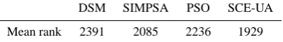
Table 4: Mean ranks of the different optimizaton method’s
performances
DSM
SIMPSA
PSO
SCE-UA
Mean rank
2391
2085
2236
1929
Table 5: p-values for pairwise Wilcoxon rank sum tests
be-tween different optimization methods
DSM
SIMPSA
PSO
SCE-UA
DSM
1
1.14
·
10
−080.0043
9.20
·
10
−18SIMPSA
1
0.0059
0.0031
PSO
1
1.08
·
10
−08SCE-UA
1
Table 6: Final parameters resulting from calibration with
OF1 found by each of the optimization methods, except for
the month of April for which the displayed minimum was
only found by PSO.
λ
κ
φ
µ
xα
ν
fitness
Jan
0.0324
0.3810
0.0593
0.9609
3.2957
0.9053
0.0345
Feb
0.0272
0.2973
0.0485
0.9483
3.4148
1.0634
0.0389
Mar
0.0327
0.5920
0.0327
1.4127
2.7201
0.1541
0.0356
Apr
0.0297
0.2918
0.0333
1.6022
3.0000
0.3353
0.0281
May
0.0257
0.1122
0.0296
3.3370
3.1148
0.4208
0.0393
Jun
0.0284
0.2003
0.0326
4.9128
3.0996
0.1899
0.0146
Jul
0.0275
0.0896
0.0268
7.4132
3.3296
0.2781
0.0134
Aug
0.0288
0.1727
0.0294
6.8543
2.8370
0.1282
0.0170
Sep
0.0266
0.1208
0.0226
3.9448
2.7106
0.2233
0.0279
Oct
0.0299
0.3523
0.0323
2.1634
2.4490
0.1775
0.0208
Nov
0.0306
0.2994
0.0490
1.1666
2.8800
0.7642
0.0365
Dec
0.0286
0.2266
0.0448
1.0846
3.1943
1.1887
0.0336
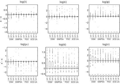
Fig. 3. Distributions of estimation error for each parameter under
different optimization methods and objective functions.
exploitative search. In this case,c2is set at 2.5, a search with an explorative character is preferred.
Figure 2b shows the results of the calibrations for different combinations ofw andc1 whenc2is fixed at 2.5. Results show that good results are obtained when the inertia weight wis kept relatively small, whilst the choice of c1 does not seem to have a profound effect on the result when using small values forw. A minimum could, however, be detected for c1=1.5 and consequently this value is chosen forc1.
Finally, Fig. 2c shows the results for different combina-tions of w andc2 withc1 fixed at 1.5. This figure shows that there is a negative correlation between both parame-ters. Higher values ofc2 in combination with lower values ofwlead to promising results, and vice versa. Because the valuec2 was previously set at 2.5, the value ofwis set at 0.4. The figure shows that for this combination good results are obtained.
In addition to the selection of the PSO parameters, sev-eral other settings have to be specified. When a population member attempts to cross parameter boundaries, that bound-ary acts as a perfect reflector. In other words, the direction of displacement of the particle is inverted in order to keep it inside the parameter boundaries.
The choice of a stopping criterion will also affect the ob-tained calibration results. In addition to the already men-tioned general stopping criteria several other approaches can be utilized for PSO. In the current paper the search procedure is stopped if the global best solutionpgdoes not change dur-ing 30 subsequent iterations. This indicates that no better
882 W. J. Vanhaute et al.: Calibration of the modified Bartlett-Lewis model
log( )λ log( )κ log( )φ
log( )μx log( )α log( )ν
x’
- x
x’
- x
OF 1 OF 2 OF 3 DSM
OF 1 OF 2 OF 3 OF 1 OF 2 OF 3 OF 1 OF 2 OF 3 SIMPSA PSO SCE-UA
OF 1 OF 2 OF 3 DSM
OF 1 OF 2 OF 3 OF 1 OF 2 OF 3 OF 1 OF 2 OF 3 SIMPSA PSO SCE-UA
OF 1 OF 2 OF 3 DSM
OF 1 OF 2 OF 3 OF 1 OF 2 OF 3 OF 1 OF 2 OF 3 SIMPSA PSO SCE-UA
OF 1 OF 2 OF 3
DSM
OF 1 OF 2 OF 3 OF 1 OF 2 OF 3 OF 1 OF 2 OF 3
SIMPSA PSO SCE-UA OF 1 OF 2 OF 3
DSM
OF 1 OF 2 OF 3 OF 1 OF 2 OF 3 OF 1 OF 2 OF 3 SIMPSA PSO SCE-UA OF 1 OF 2 OF 3
DSM
OF 1 OF 2 OF 3 OF 1 OF 2 OF 3 OF 1 OF 2 OF 3 SIMPSA PSO SCE-UA
Fig. 4: Distributions of estimation error for each parameter under different optimization methods and objective functions.
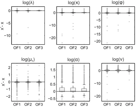
[image:10.595.87.510.62.357.2]Fig. 5: Distributions of estimation error for each parameter, grouped according to the used objective function.
Fig. 4. Distributions of estimation error for each parameter, grouped according to the used objective function.
solutions are being found. This criterion is preferred against a convergence criterion, i.e. a certain fraction of the popu-lation has to converge to the same solution in order for the algorithm to stop, because, from personal experience, it has become clear that the latter is quite time consuming. 5.3 Shuffled complex evolution
The parameters of the SCE-UA algorithm have been set to their recommended values (Duan et al., 1994), except for the number of complexespand the number of inner loop itera-tionsnIwhich are evaluated more closely. The value ofpis recommended to lie between 2 and 20. Thereforepis evalu-ated at different values within this interval. It is expected that the use of more complexes will lead to better results, but at a higher computational cost. The number of inner loop iter-ations will also have an influence on the results. The higher the number of inner loop iterations, the better the offspring that is being generated (the simplex will be able to progress further towards an optimum), again, bearing in mind the aug-mented computational burden. The parameter search thus seeks to find a good balance between results and efficiency. The procedure is the same as with PSO and SIMPSA. For ev-ery combination of SCE-UA parameters calibrations are con-ducted for each month. Those results are averaged and dis-played in Fig. 3. These results confirm that a higher number of complexes leads to better results, as does a higher
num-ber of inner loop iterations. The numnum-ber of complexes p, however, is best set at 5, since for this value good results are obtained throughout and this is less computationally expen-sive than 10 or 20 complexes. The value ofnI is chosen as 20. It can be seen in Fig. 3 that for this value better results are obtained than is the case whennIwould be equal to 10 or 30, and the results are equal to those obtained whennI >30, howevernI=20 is computationally more efficient.
6 Comparison of optimization methods
After successfully implementing the presented optimization methods, the calibration of the MBL model can be per-formed. The performance of the optimization methods is evaluated in two steps. First, a known parameter set is used to perform several simulations to which the MBL model will be fitted using the different optimization methods and ob-jective functions. This way, the optimization methods and the objective functions’ ability to retrieve a known parame-ter set will be assessed. Second, the MBL model is fitted to the observations at Uccle for each optimization method and objective function.
W. J. Vanhaute et al.: Calibration of the modified Bartlett-Lewis model 883
log( )λ log( )κ log( )φ
log( )μx log( )α log( )ν
x’
- x
x’
- x
OF 1 OF 2 OF 3
DSM
OF 1 OF 2 OF 3 OF 1 OF 2 OF 3 OF 1 OF 2 OF 3
SIMPSA PSO SCE-UA
OF 1 OF 2 OF 3
DSM
OF 1 OF 2 OF 3 OF 1 OF 2 OF 3 OF 1 OF 2 OF 3
SIMPSA PSO SCE-UA
OF 1 OF 2 OF 3
DSM
OF 1 OF 2 OF 3 OF 1 OF 2 OF 3 OF 1 OF 2 OF 3
SIMPSA PSO SCE-UA
OF 1 OF 2 OF 3
DSM
OF 1 OF 2 OF 3 OF 1 OF 2 OF 3 OF 1 OF 2 OF 3
SIMPSA PSO SCE-UA
OF 1 OF 2 OF 3
DSM
OF 1 OF 2 OF 3 OF 1 OF 2 OF 3 OF 1 OF 2 OF 3
SIMPSA PSO SCE-UA
OF 1 OF 2 OF 3
DSM
OF 1 OF 2 OF 3 OF 1 OF 2 OF 3 OF 1 OF 2 OF 3
SIMPSA PSO SCE-UA
Fig. 4: Distributions of estimation error for each parameter under different optimization methods and objective functions.
Fig. 5: Distributions of estimation error for each parameter, grouped according to the used objective function.
Fig. 5. Distributions of estimation error for each parameter, grouped
according to the used optimization method.
6.1 Retrieval of known parameters
To assess the ability of the optimization methods the objec-tive functions to retrieve a known parameter set, a parameter set was taken from Verhoest et al. (1997) to perform a total of 400 simulations with the MBL model. The length of each simulation is equal to 105 yr. Afterwards, the MBL model was fitted to these simulations. For each objective function, and for each optimization method, 400 calibrations were car-ried out, i.e. only one repetition of the calibration for each simulated data set. Ideally, each of these calibrations should result in the retrieval of the known parameter set. However, since this is very unlikely, the distribution of estimation er-rors will shed light on the algorithms and objective functions’ performance in their attempt to retrieve known parameters.
Figure 4 visualises the distribution of the estimation er-rors on the six MBL model parameters for the month of Jan-uary. It can be seen that SIMPSA, PSO, and SCE-UA per-form better in identifying the true parameters in comparison with the DSM with multiple starting points. Significant dif-ferences between the former optimization methods, or be-tween the objective functions, are not clearly visible. To fa-cilitate this, the calibration results are grouped according to the objective function with which they were obtained, regard-less of the used optimization method (see Fig. 5). Similarly, Fig. 6 displays the distribution of the estimation error in func-tion of the used optimizafunc-tion method, regardless of the used objective function.
Figure 5 indicates that the use of OF3 might lead to bet-ter identifiability (this is especially visible forα), however differences are very small.
[image:11.595.50.287.63.249.2]As for the ability of the optimization methods to identify the true parameters, Fig. 6 confirms the DSM’s inability to do so. SIMPSA seems to lead to very large estimation errors
Table 3. Descriptive statistics of the performance of different
opti-mization methods for the calibration of the Modified Bartlett-Lewis Rectangular Pulses model.
minimum median StDev duration (min)
DSM OF1 0.0300 0.0467 0.0247 9 OF2 0.0594 0.0922 0.0580 15 OF3 0.1908 0.2063 0.0524 9
SIMPSA OF1 0.0300 0.0300 0.4696 18 OF2 0.0594 0.0594 18.2159 100 OF3 0.1908 0.1908 0.6206 4
PSO OF1 0.0283 0.0311 0.1531 13 OF2 0.0594 0.0624 0.8168 31 OF3 0.1908 0.1908 0.2359 14
SCE-UA OF1 0.0300 0.0300 0.1150 14 OF2 0.0594 0.0594 0.3552 24 OF3 0.1908 0.1908 0.3433 11
on several occasions. PSO seems to be the most consistent in identifying the true parameter, however, its results are com-parable to those of SCE-UA, apart from a few outliers. 6.2 Fit to Uccle data
To evaluate the performance of the different optimization methods and objective functions in a realistic situation, 30 repetitions of the calibration are performed for each opti-mization method, each objective function, and each month. The 30 repetitions vary in that for each of them, the algo-rithm starts from a different initial situation. For the DSM, PSO, and SCE-UA, the initial population is chosen randomly within the preset parameter boundaries according to a uni-form distribution. Similarly, the initial simplex for SIMPSA is created around a randomly chosen point in parameter space, also sampled from a uniform distribution.
In order to compare the performance of the used optimiza-tion methods, several approaches can be adopted. Here, we will first summarize the obtained results by a set of descrip-tive statistics. This will give a first indication of how well certain methods perform compared with the others. Table 3 displays the aforementioned descriptive statistics for the dif-ferent objective functions, fitted by the difdif-ferent optimiza-tion methods. The minimum and median values and the standard deviation (StDev) of the objective function values obtained after 30 repetitions, displayed in Table 3 are cal-culated by, first, determining those statistics for each month separately and, second, taking the mean over 12 months. The results are displayed in such a way to enhance interpreta-tion without loss of generality. The durainterpreta-tion of the calibra-tion is the mean duracalibra-tion of the total calibracalibra-tion procedure, i.e. taking into account all of the 12 months, on a PC with an Intel®Core™i7-2600 CPU at 3.40 GHZ. All software is implemented in Matlab®.
[image:11.595.308.548.110.266.2]884 W. J. Vanhaute et al.: Calibration of the modified Bartlett-Lewis model DSM SIMPSA PSO SCE-UA DSM SIMPSA PSO SCE-UA DSM SIMPSA PSO SCE-UA DSM SIMPSA PSO SCE-UA DSM SIMPSA PSO SCE-UA DSM SIMPSA PSO SCE-UA
Fig. 6: Distributions of estimation error for each parameter, grouped according to the used optimization method.
Fig. 6. Box plots comparing calibration results of DSM, SIMPSA,
PSO and SCE-UA. All months and repetitions are lumped together, no averages have been taken.
Several observations can be made on the basis of Table 3. First, it seems that the obtained minima for the different ob-jective functions are largely the same. This means that, when the optimization is repeated at least 30 times, each of the optimization methods is able to find the same minima. Fur-ther inspection of these minima indicates they result from the same minimizers, i.e. the same parameter combinations are being found by the different optimization methods. This sug-gests that the parameters are highly identifiable, seeing that the same minima are being found by independent optimiza-tion methods. This evidence is corroborated by the fact that the median values, at least for SIMPSA and SCE-UA, are equal to the minima, i.e. the same points are being withheld as the minimum in the majority of the calibration runs. As for DSM and PSO, the median values are fairly close to the minimum. Thus, when it comes to finding a suitable mini-mum, DSM, SIMPSA, PSO and SCE-UA are almost inter-changeable. All four are able to locate the same minima on multiple occasions. Note that PSO is able to find a minimum with a lower objective function value for OF1, in compar-ison with SIMPSA and SCE-UA. Yet the value reported in Table 3 is the mean value of the minima of the 12 different months. Further investigation of the data uncovers that for the month of April, PSO attained a better solution, however, the differences in the parameter values are rather small, so it is doubtful that it will lead to significant differences in the simulations.
Second, the robustness of each optimization method can be judged in several ways. A first indicator is the standard deviation of the objective function values of the found min-ima after 30 repetitions. Clearly, DSM is far more robust (i.e. by an order of magnitude) than the other optimization
20 W. J. Vanhaute et al.: Calibration of the modified Bartlett-Lewis model
(a) OF1
DSM SIMPSA PSO SCE−UA
0 0.2 0.4 0.6 0.8 1
Objective function value OF2
(b) OF2
DSM SIMPSA PSO SCE−UA
0.5 1 1.5
Objective function value OF3
(c) OF3
Fig. 7: Box plots comparing calibration results of DSM, SIMPSA, PSO and SCE-UA. All months and repetitions are lumped together, no averages have been taken.
0.0130 0.014 0.015 0.016 0.017
0.2 0.4 0.6 0.8 1
rainfall depth (mm)
F(x)
Mean 10 minute rainfall depth in January
eCDF OF1 simulations Observation (Uccle)
Fig. 8: Empirical Cumulative distribution function of the mean 10 minute rainfall depth in January as simulated with OF1 vs. observed value
0 1 2 3 4
0 0.2 0.4 0.6 0.8 1
rainfall depth (mm)
F(x)
12 hour autocovariance in March
eCDF OF1 simulations Observation (Uccle)
Fig. 9: Empirical Cumulative distribution function of the lag-1 autocovariance of the lag-12 hourly-rainfall depth in March as simulated with OF1 vs. observed value
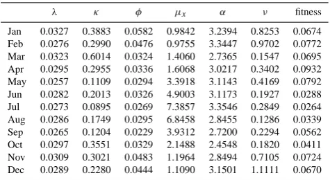
Table 7: Final parameters resulting from calibration with OF2 found by each of the optimization methods.
λ κ φ µx α ν fitness
Jan 0.0327 0.3883 0.0582 0.9842 3.2394 0.8253 0.0674 Feb 0.0276 0.2990 0.0476 0.9755 3.3447 0.9702 0.0772 Mar 0.0323 0.6014 0.0324 1.4060 2.7365 0.1547 0.0695 Apr 0.0295 0.2955 0.0336 1.6068 3.0217 0.3402 0.0932 May 0.0257 0.1109 0.0294 3.3918 3.1143 0.4169 0.0792 Jun 0.0282 0.2013 0.0326 4.9003 3.1173 0.1927 0.0288 Jul 0.0273 0.0895 0.0269 7.3857 3.3546 0.2849 0.0264 Aug 0.0286 0.1749 0.0295 6.8458 2.8455 0.1286 0.0339 Sep 0.0265 0.1204 0.0229 3.9312 2.7200 0.2294 0.0562 Oct 0.0297 0.3551 0.0329 2.1488 2.4548 0.1820 0.0411 Nov 0.0309 0.3021 0.0483 1.1964 2.8494 0.7105 0.0724 Dec 0.0289 0.2280 0.0444 1.1090 3.1501 1.1111 0.0670
20 W. J. Vanhaute et al.: Calibration of the modified Bartlett-Lewis model
(a) OF1
DSM SIMPSA PSO SCE−UA
0 0.2 0.4 0.6 0.8 1
Objective function value OF2
(b) OF2
DSM SIMPSA PSO SCE−UA
0.5 1 1.5
Objective function value OF3
(c) OF3
Fig. 7: Box plots comparing calibration results of DSM, SIMPSA, PSO and SCE-UA. All months and repetitions are lumped together, no averages have been taken.
0.0130 0.014 0.015 0.016 0.017
0.2 0.4 0.6 0.8 1
rainfall depth (mm)
F(x)
Mean 10 minute rainfall depth in January
eCDF OF1 simulations Observation (Uccle)
Fig. 8: Empirical Cumulative distribution function of the mean 10 minute rainfall depth in January as simulated with OF1 vs. observed value
0 1 2 3 4
0 0.2 0.4 0.6 0.8 1
rainfall depth (mm)
F(x)
12 hour autocovariance in March
eCDF OF1 simulations Observation (Uccle)
Fig. 9: Empirical Cumulative distribution function of the lag-1 autocovariance of the lag-12 hourly-rainfall depth in March as simulated with OF1 vs. observed value
Table 7: Final parameters resulting from calibration with OF2 found by each of the optimization methods.
λ κ φ µx α ν fitness
Jan 0.0327 0.3883 0.0582 0.9842 3.2394 0.8253 0.0674 Feb 0.0276 0.2990 0.0476 0.9755 3.3447 0.9702 0.0772 Mar 0.0323 0.6014 0.0324 1.4060 2.7365 0.1547 0.0695 Apr 0.0295 0.2955 0.0336 1.6068 3.0217 0.3402 0.0932 May 0.0257 0.1109 0.0294 3.3918 3.1143 0.4169 0.0792 Jun 0.0282 0.2013 0.0326 4.9003 3.1173 0.1927 0.0288 Jul 0.0273 0.0895 0.0269 7.3857 3.3546 0.2849 0.0264 Aug 0.0286 0.1749 0.0295 6.8458 2.8455 0.1286 0.0339 Sep 0.0265 0.1204 0.0229 3.9312 2.7200 0.2294 0.0562 Oct 0.0297 0.3551 0.0329 2.1488 2.4548 0.1820 0.0411 Nov 0.0309 0.3021 0.0483 1.1964 2.8494 0.7105 0.0724 Dec 0.0289 0.2280 0.0444 1.1090 3.1501 1.1111 0.0670
Fig. 7. Empirical Cumulative distribution function of the mean
10 min rainfall depth in January as simulated with OF1 vs. observed value.
methods. When comparing the remaining three methods, it can be seen that PSO and SCE-UA have resulted in roughly the same standard deviations, whereas SIMPSA clearly had problems in minimizing OF2. It shows a much higher stan-dard deviation for OF2, and moreover, the average duration