Machine learning CICY threefolds

      

City, University of London Institutional Repository

Citation:

Bull, K., He, Y. ORCID: 0000-0002-0787-8380, Jejjala, V. and Mishra, C. (2018).

Machine learning CICY threefolds. Physics Letters, Section B: Nuclear, Elementary Particle

and High-Energy Physics, 785, pp. 65-72. doi: 10.1016/j.physletb.2018.08.008

This is the accepted version of the paper.

This version of the publication may differ from the final published

version.

Permanent repository link:

http://openaccess.city.ac.uk/20647/

Link to published version:

http://dx.doi.org/10.1016/j.physletb.2018.08.008

Copyright and reuse: City Research Online aims to make research

outputs of City, University of London available to a wider audience.

Copyright and Moral Rights remain with the author(s) and/or copyright

holders. URLs from City Research Online may be freely distributed and

linked to.

Contents lists available atScienceDirect

Physics

Letters

B

www.elsevier.com/locate/physletb

Machine

learning

CICY

threefolds

Kieran Bull

a

,

∗

,

Yang-Hui He

b

,

c

,

d

,

Vishnu Jejjala

e

,

Challenger Mishra

f

a_{DepartmentofPhysics,UniversityofOxford,UK} b_{DepartmentofMathematics,CityUniversity,London,UK} c_{SchoolofPhysics,NanKaiUniversity,Tianjin,PRChina} d_{MertonCollege,UniversityofOxford,UK}

e_{MandelstamInstituteforTheoreticalPhysics,NITheP,CoE-MaSS,andSchoolofPhysics,UniversityoftheWitwatersrand,SouthAfrica} f_{RudolfPeierlsCentreforTheoreticalPhysicsandChristChurch,UniversityofOxford,UK}

a

r

t

i

c

l

e

i

n

f

o

a

b

s

t

r

a

c

t

Articlehistory: Received2July2018

Receivedinrevisedform1August2018 Accepted7August2018

Availableonline16August2018 Editor:M.Cvetiˇc

Keywords: Machinelearning Neuralnetwork SupportVectorMachine Calabi–Yau

Stringcompactifications

ThelatesttechniquesfromNeuralNetworksandSupportVectorMachines(SVM)areusedtoinvestigate geometric properties ofComplete Intersection Calabi–Yau (CICY)threefolds, aclass ofmanifolds that facilitatestringmodelbuilding.AnadvancedneuralnetworkclassifierandSVMareemployedto(1)learn Hodgenumbersandreportaremarkableimprovementoverpreviousefforts,(2)queryforfavourability, and (3) predict discrete symmetries,a highly imbalancedproblem to whichboth SyntheticMinority OversamplingTechnique (SMOTE)and permutationsoftheCICYmatrixare used todecreasetheclass imbalanceandimproveperformance.Ineachcasestudy,weemployageneticalgorithmtooptimisethe hyperparametersofthe neuralnetwork. Wedemonstratethat ourapproach providesquickdiagnostic toolscapableofshortlistingquasi-realisticstringmodelsbasedoncompactificationoversmoothCICYs and further supports the paradigm that classes of problems in algebraicgeometry can be machine learned.

©2018PublishedbyElsevierB.V.ThisisanopenaccessarticleundertheCCBYlicense (http://creativecommons.org/licenses/by/4.0/).FundedbySCOAP3.

1. Introduction

Stringtheorysuppliesaframeworkforquantumgravity.Finding ouruniverseamongthemyriadofpossible,consistentrealisations ofafourdimensionallow-energylimitofstringtheoryconstitutes the vacuum selection problem. Most of the vacua that populate the string landscapeare false inthat they lead to physics vastly differentfrom what we observe in Nature. We have so far been unable to construct even one solution that reproduces all of the known features of particle physics and cosmology in detail. The challenge ofidentifying suitable string vacua isa problemin big datathatinvitesamachinelearningapproach.

The useof machine learning to studythe landscape ofvacua is a relatively recent development. Several avenueshave already yielded promising results. These include Neural Networks [1–4], LinearRegression[5],LogisticRegression[5,4],LinearDiscriminant Analysis,k-NearestNeighbours,ClassificationandRegressionTree,

*

Correspondingauthor.

E-mailaddresses:kieran.bull@seh.ox.ac.uk(K. Bull),hey@maths.ox.ac.uk (Y.-H. He),vishnu@neo.phys.wits.ac.za(V. Jejjala),challenger.mishra@gmail.com (C. Mishra).

Naive Bayes [5], Support Vector Machines [5,4], Evolving Neural Networks[6], GeneticAlgorithms[7], DecisionTreesandRandom Forest[4],NetworkTheory[8].

Calabi–Yauthreefoldsoccupyacentralrôleinthestudyofthe string landscape. In particular, Standard Model like theories can beengineeredfromcompactificationonthesegeometries.Assuch, Calabi–Yaumanifoldshavebeenthesubjectofextensivestudyover thepastthreedecades.Vastdatasetsoftheirpropertieshavebeen constructed,warrantingadeep-learningapproach[1,2],whereina paradigm of machine learning computational algebraic geometry hasbeenadvocated.Inthispaper,weemploy feedforwardneural networksandsupportvectormachinestoprobeasubclassofthese manifolds to extract topological quantities. We summarise these techniquesbelow.

•

Inspiredbytheir biologicalcounterparts,artificialNeural Net-worksconstituteaclassofmachinelearningtechniques capa-bleofdealingwithbothclassificationandregressionproblems. Inpractice,theycanbethoughtofashighlycomplexfunctions actingonan input vectorto producean outputvector. There areseveraltypesofneuralnetworks,butinthisworkwe em-ployfeedforwardneuralnetworks,whereininformationmoves

https://doi.org/10.1016/j.physletb.2018.08.008

66 K. Bull et al. / Physics Letters B 785 (2018) 65–72

inthe forward directionfromthe input nodes tothe output nodesviahiddenlayers.

•

SupportVectorMachines(SVMs), in contrast to neural net-works, take a moregeometric approach tomachine learning. SVMsworkbyconstructinghyperplanesthatpartitionthe fea-turespace andcan be adapted to act asboth classifiers and regressors.

The manifolds of interest to us are the Complete Intersection Calabi–Yau threefolds (CICYs), which we review in the following section. TheCICYs generalisethe famous quintic aswell asYau’s constructionoftheCalabi–Yau threefoldembedded in

P

3

×

P

3 [9]. Thesimplicityoftheir description makesthisclass ofgeometries particularlyamenabletothetoolsofmachinelearning.Thechoice ofCICYsis howevermainlyguided by other considerations.First, theCICYsconstitute asizeable collectionofCalabi–Yau manifolds andare infactthe firstsuch large datasetinalgebraic geometry. Second, many properties of the CICYs have already been com-putedovertheyears,liketheirHodgenumbers[9,10] anddiscrete isometries[11–14].TheHodgenumbersoftheirquotientsbyfreely actingdiscreteisometrieshavealsobeencomputed[11,15–18].In addition,theCICYsprovideaplaygroundforstringmodelbuilding. Theconstructionofstableholomorphicvector[19–23] andmonad bundles[21] over smooth favourableCICYs has produced several quasi-realisticheteroticstringderivedStandardModelsthrough in-termediate GUTs.Theseconstituteanother largedatasetbasedon thesemanifolds.

Furthermore,theHodgenumbersofCICYswererecentlyshown tobemachinelearnabletoareasonabledegreeofaccuracyusinga primitiveneuralnetworkofthemulti-layerperceptrontype[1].In thispaper,weconsider whethera morepowerfulmachine learn-ing tool (like a more complexneural network oran SVM)yields significantly betterresults.We wish tolearn theextent towhich such topological properties of CICYsare machine learnable, with theforesightthatmachinelearningtechniquescanbecomea pow-erfultoolinconstructingevermorerealisticstringmodels,aswell ashelpingunderstandCalabi–Yaumanifoldsintheirownright. Ex-panding upon the primitive neural network in [1], and withthe foresightthatlargedatasetswilllikelybenefitfromdeeplearning, weturntoneuralnetworks.Wechoosetocontrastthistechnique with SVMs, which are particularly effective for smaller datasets withhighdimensionaldata,suchasthedatasetofCICYthreefolds. Guided by these considerations, we conduct three case stud-ies over theclass of CICYs.We first apply SVMsand neural net-workstomachinelearntheHodgenumberh1,1 _{ofCICYs.Wethen}

attempt to learn whether a CICY is favourably embedded in a product ofprojective spaces,andwhethera given CICYadmitsa quotientbyafreelyactingdiscretesymmetry.

The paperisstructured asfollows.In Section 2,we providea briefoverviewofCICYsandthedatasetsoverthemrelevanttothis work.InSection3,wediscussthemetricsforourmachinelearning paradigms.Finally,inSection4,wepresentourresults.

2. TheCICYdataset

ACICYthreefoldisaCalabi–Yaumanifoldembeddedina prod-uctofcomplexprojectivespaces,referredtoastheambientspace. Theembeddingisgivenbythezerolocusofasetofhomogeneous polynomialsoverthecombinedsetofhomogeneouscoordinatesof theprojectivespaces.ThedeformationclassofaCICYisthen cap-turedbyaconfigurationmatrix(1),whichcollectsthemulti-degrees ofthepolynomials:

X

=

P

n1

..

.

P

nm

⎡

⎢

⎢

⎢

⎣

q1₁

. . .

q1_K

..

.

. .

.

..

.

qm₁

. . .

qm_K

⎤

⎥

⎥

⎥

⎦

,

qra

∈

Z

≥0

.

(1)

Inorder forthe configurationmatrixin(1) todescribe aCICY threefold, we requirethat

_rnr

−

K

=

3.In addition,the

vanish-ing of the first Chern class is accomplished by demanding that

aqra

=

nr

+

1,foreachr

∈ {

1

,

. . . ,

m

}

.Thereare7890 CICY

config-urationmatricesintheCICYlist(availableonlineat[24]).Atleast 2590 oftheseareknowntobedistinctasclassicalmanifolds.

The Hodge numbers hp,q _{of a Calabi–Yau manifold are the}

dimensions of its Dolbeault cohomology classes Hp,q_{. A related}

topologicalquantityistheEulercharacteristic

χ

.Wedefinethese quantitiesbelow:

hp,q

=

dimHp,q

,

χ

=

3

p,q=0

(

−

1

)

p+qhp,q

,

p,q

∈ {

0

,

1

,

2

,

3

}

(2)

For a smooth and connected Calabi–Yau threefold with holon-omy group SU

(

3

)

, the only unspecified Hodge numbers are h1,1

and h2,1_{. These are topological invariants that capture the}

di-mensionsoftheKählerandthecomplexstructure modulispaces, respectively. The Hodge numbers of all CICYs are readily acces-sible [24]. There are 266 distinct Hodge pairs

(

h1,1

_,

_h2,1

₎

_{of the}

CICYs,with0

≤

h1,1

_≤

_{19 and0}

_≤

_h2,1

_≤

_{101.Fromamodel}

build-ingperspective,knowledgeoftheHodgenumbersisimperativeto theconstructionofastringderivedStandardModel.

If the entire second cohomology class of the CICY descends fromthatoftheambientspace

A

=

P

n1

×

_{. . .}

×

P

nm_,thenwe iden-tifythe CICYasfavourable.There are 4874 favourableCICYs [24]. As an aside, we note that it was shown recently that all but 48 CICY configuration matrices can be brought to a favourable formthroughineffectivesplittings[25].The remainingcanbe seen to be favourably embedded in a product of del Pezzo surfaces. The favourable CICYlistis also available online[26], although in this paper we will not be concerned withthis new list of CICY configurationmatrices. ThefavourableCICYs havebeenespecially amenable to the construction of stable holomorphic vector and monad bundles, leading to several quasi-realistic heterotic string models.

Discrete symmetries are one of thekey componentsof string model building. The breaking of the GUT group to the Standard ModelgaugegroupproceedsviadiscreteWilsonlines,andassuch requires a non-simply connectedcompactification space. Prior to theclassificationefforts[11,12],almostallknownCalabi–Yau man-ifoldsweresimplyconnected.Theclassificationresultedin identi-fyingallCICYsthatadmit aquotientbyafreely actingsymmetry, totalling195 innumber,2

.

5%ofthetotal,creatingahighly unbal-anceddataset.31 distinctsymmetrygroupswerefound,thelargest beingoforder32.Countinginequivalentprojectiverepresentations of the various groups acting on the CICYs, a total of 1695 CICY quotientswereobtained[24].

groundsthat thesizeofthedatasetisitselfmuchlargerthanthe latterdataset.

3. Benchmarkingmodels

Inorder to benchmarkand comparethe performance of each machine learning approach we adapt inthis work, we use cross validation and a range of other statistical measures. Cross vali-dation meanswe take ourentiredata set andsplit itinto train-ing and validation sets. The training set is used to train models whereasthevalidationsetremainsentirelyunseenbythemachine learning algorithm. Accuracy measures computed on the training setthusgiveanindicationofthemodel’sperformanceinrecalling what it has learned. More importantly, accuracy measures com-putedagainst the validationset give an indication ofthe models performanceasapredictor.

Forregressionproblemswemakeuseofbothrootmeansquare error(RMS)andthecoefficientofdetermination(R2)toassess per-formance: RMS

:=

1 N N

i=1

(

y_ipred

−

yi

)

2

)

1/2

,

R2

:=

1

−

i

(

yi

−

yipred

)

2

i

(

yi

− ¯

y)2

,

(3)

where yi and ypredi stand foractual andpredictedvalues,withi

takingvalues in 1 to N, and y

¯

stands forthe average of all yi.

Arudimentarybinaryaccuracy isalsocomputedby roundingthe predictedvalue and counting the results in agreement with the data.As thisaccuracy is a binary success orfailure, we can use thismeasuretocalculateaWilsonconfidenceinterval.Define

ω

±

:=

p

+

z2

2n

1

+

z_n2

±

z

1

+

z_n2

p(1

−

p)

n

+

z2

4n2

1/2

,

(4)

wherepistheprobabilityofasuccessfulprediction,nthenumber ofentriesinthedataset,andztheprobitofthenormaldistribution (e.g., fora 99% confidenceinterval, z

=

2

.

575829).The upperand thelower bounds ofthisinterval are denoted by WUB andWLB respectively.

Forclassifiers, we haveaddressed two distinct types of prob-lems in this paper, namely balanced and imbalanced problems. Balancedproblemsarewherethenumberofelements inthetrue andfalse classesare comparableinsize.Imbalancedproblems,or thesocalledneedleinahaystack,aretheoppositecase.Itis impor-tanttomakethisdistinction,sincemodelstrainedonimbalanced problemscan easily achieve a highaccuracy, butaccuracywould be a meaningless metric in this context. For example, consider the case where only

∼

0

.

1% of the data is classified as true. In minimisingits cost function on training, a neural network could naivelytrainamodelwhichjustpredictsfalseforanyinput.Such amodelwouldachievea99

.

9% accuracy,butitisuselessinfinding thespecialfewcasesthatweareinterestedin.Adifferentmeasure isneededinthesecases.Forclassifiers,thepossibleoutcomesare summarisedbytheconfusionmatrixofTable1,whoseelementswe usetodefineseveralperformancemetrics:

TPR

:=

tp

tp

+

f n

,

FPR

:=

f p

f p

+

tn

,

(5)

Accuracy

:=

tp

+

tn

tp

+

tn

+

f p

+

f n

,

Precision

:=

[image:4.612.310.562.93.136.2]

tp tp

+

f p

,

Table 1

Confusionmatrix.

Actual

True False

Predicted True True Positive (tp) False Positive (f p) Classification False False Negative (f n) True Negative (tn)

where, TPR (FPR) stand for True (False) Positive Rate, the for-mer also known as recall. For balanced problems, accuracy is the go-to performance metric, along with its associated Wilson confidence interval. However, for imbalanced problems, we use F-valuesand AUC.Wedefine,

F

:=

2

1

Recall

+

Precision1

,

(6)

while AUC is the area under the receiver operatingcharacteristic (ROC)curvethatplotsTPRagainstFPR. F-valuesvaryfrom0 to 1, whereasAUCrangesfrom0

.

5 to 1.Wewilldiscusstheseingreater detailinSection4.3.2.

4. Casestudies

Weconduct threecasestudiesoverthe CICYthreefolds.Given aCICYthreefold X,weexplicitlytrytolearnthetopological quan-tityh1,1

(

X

)

,theHodgenumberthatcapturesthedimensionofthe Kählerstructuremodulispaceof X.Wethenattempta(balanced) binary query, asking whethera given manifold is favourable. Fi-nally, we attemptan (imbalanced)binary queryaboutwhethera CICY threefold X, admitsa quotient X

/

G by a freely acting dis-crete isometry group G. In all the case studies that follow, neu-ral networkswere implemented using the Keras Python package withTensorFlow backend. SVMswere implemented by using the quadratic programmingPythonpackage Cvxopt to solve theSVM optimisationproblem.

4.1. MachinelearningHodgenumbers

AsnotedinSection2,theonlyindependentHodgenumbersof a Calabi–Yau threefold areh1,1 andh2,1. We attempttomachine learnthese.Foragivenconfigurationmatrix(1) describingaCICY, theEuler characteristic

χ

=

2

(

h1,1

₋

_h2,1

₎

_{canbe computedfrom}

asimplecombinatorialformula[27]. Thus,itissufficienttolearn onlyone oftheHodge numbers.Wechooseto learnh1,1 _{since it}

takesvaluesinasmallerrangeofintegersthanh2,1_.

4.1.1. Architectures

To determine theHodge numbers we use regressionmachine learning techniquestopredict acontinuous outputwiththeCICY configuration matrix (1) as the input. The optimal SVM hyper-parameters were found by hand to be a Gaussian kernel with

σ

=

2

.

74, C

=

10, and

=

0

.

01. Optimal neural network hyper-parameters were found with a genetic algorithm, leading to an overallarchitecture offivehiddenlayerswith876,461,437,929, and 404 neurons, respectively. The algorithm also found that a ReLU (rectified linear unit) activation layer and dropout layer of dropout0

.

2072 betweeneachneuronlayergiveoptimalresults.

A neural network classifier was also used. To achieve this, ratherthanusingoneoutputlayerasisthecaseforabinary clas-sifierorregressor,weusean outputlayerwith20 neurons(since h1,1

_∈

₍

₀

_,

₁₉

₎

_{) witheach neuron mappingto 0}

_/

_{1, the location of}

the1 correspondingtoauniqueh1,1 _{value.Notethisiseffectively}

[image:5.612.63.257.67.226.2]

68 K. Bull et al. / Physics Letters B 785 (2018) 65–72

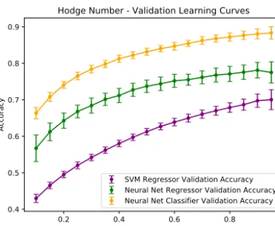
Fig. 1.Hodge learningcurvesgeneratedbyaveraging over100 differentrandom cross validationsplits usinga cluster. The accuracy quotedfor the 20 channel (sinceh1,1_{∈ [0}

,19])neuralnetworkclassifierisforcompleteagreementacrossall 20 channels.

training data (choose the output to be the largest h1,1 _fromthe

training data — fora large enough sample it islikely to contain h1,1

₌

_{19).Moreover,forasmalltrainingdatasize,ifonlyh}1,1

val-ueslessthan agivennumber arepresentinthe data,themodel will notbe ableto learn theseh1,1 _{valuesanyway —this would}

happenwithacontinuousoutputregressionmodelaswell. Thegeneticalgorithm isusedtofindthe optimalclassifier ar-chitecture. Surprisingly, it finds that adding several convolution layers led tothe best performance. Thisis unexpected as convo-lution layers look for features which are translationally or rota-tionally invariant (for example, in number recognition they may learntodetectroundededgesandassociatethiswithazero).Our CICYconfigurationsmatricesdonotexhibitthesesymmetries,and thisistheonlyresultinthepaperwhereconvolution layerslead tobetter resultsrather thanworse. The optimalarchitecture was foundtobebefourconvolutionlayerswith57,56,55,and43 fea-turemaps,respectively,allwithakernelsizeof3

×

3.Theselayers werefollowedbytwohiddenfullyconnectedlayersandtheoutput layer,thehiddenlayerscontaining169 and491 neurons.ReLU ac-tivationsandadropoutof0

.

5 wereincludedbetweeneverylayer, withthelastlayerusingasigmoidactivation.Trainingwitha lap-topcomputer’s1 _{CPUtook lessthan10minutesandexecutionon}

thevalidationsetaftertrainingtakesseconds.

4.1.2. Outcomes

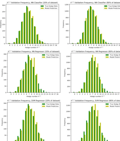
Our results are summarised in Figs. 1 and 2 and in Table 2. Clearly, the validation accuracy improves as the training set in-creases in size. The histograms in Fig. 2 show that the model slightlyoverpredictsatlargervaluesofh1,1.

Wecontrastourfindingswiththepreliminaryresultsofa pre-viouscasestudybyoneoftheauthors[1,2] inwhicha Mathemat-icaimplementedneuralnetworkofthemulti-layerperceptrontype wasusedto machinelearnh1,1_{.Inthiswork, atrainingdatasize}

of0

.

63 (5000)wasused,andatestaccuracyof77% wasobtained. Note thisaccuracy is against theentire dataset afterseeing only thetrainingset,whereaswecomputevalidationaccuraciesagainst only the unseen portion after training. In [1] there were a total of1808 errors,soassumingthetrainingsetwasperfectlylearned (reasonableastrainingaccuracycanbearbitrarilyhighwith over-fitting), this translates to a validation accuracy of 0

.

37. For the samesized crossvalidation split,we obtaina validationaccuracy of0

.

81

±

0

.

01,a significantenhancement. Moreover,it shouldbe

1 _{Laptopspecs:LenovoY50,i7-4700HQ,2.4 GHzquadcore;16 GBRAM.}

emphasized thatwhereas [1,2] did abinary classification oflarge vs. small Hodge numbers, herethe actual Hodge number h1,1 _is

learned,whichisamuchmoresophisticatedtask.

4.2. Machinelearningfavourableembeddings

Following fromthe discussioninSection 2,we nowstudythe binary query:givena CICYthreefoldconfigurationmatrix(1),can we deduce iftheCICYis favourablyembedded in theproduct of projective spaces? Already we could attemptto predict ifa con-figuration isfavourablewiththeresultsofSection 4.1by predict-ingh1,1 _{explicitlyandcomparingittothenumberofcomponents}

of

A

.However,werephrasetheproblemasabinaryquery,taking theCICYconfigurationmatrixastheinputandreturn0 or1 asthe output.

AnoptimalSVMarchitecturewasfoundbyhandtousea Gaus-siankernelwith

σ

=

3 andC

=

0.Neuralnetworkarchitecturewas alsofound byhand,asasimpleonehiddenlayerneural network with 985 neurons,ReLU activation, dropoutof 0

.

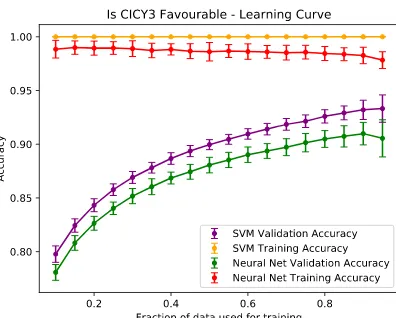
46, andsigmoid activationattheoutputlayergavebestresults.

Results are summarised inFig.3 andTable 3.Remarkably, af-ter seeingonly 5% of thetraining data (400 entries), the models are capable of extrapolating to the full dataset withan accuracy

∼

80%.Thisanalysistooklessthanaminuteonalaptopcomputer. SincecomputingtheHodgenumbersdirectlywasatime consum-ing and nontrivialproblem[27],this isa prime exampleof how applying machinelearning could shortlistdifferent configurations for further study in the hypothetical situation of an incomplete dataset.

4.3. Machinelearningdiscretesymmetries

The symmetry data resulting from the classifications [11,12] presents variouspropertiesthat we can tryto machinelearn. An idealmachinelearningmodelwouldbeabletoreplicatethe classi-ficationalgorithm,givingusalistofeverysymmetrygroupwhich is a quotientfor a givenmanifold. However, thisis a highly im-balancedproblem,asonlyatinyfractionofthe7890 CICYswould admit a specificsymmetry group.Thus, we firsttrya morebasic question,givenaCICYconfiguration,canwepredictiftheCICY ad-mits anyfreely actinggroup. Thisisstill mostdefinitely a needle inahaystackproblemasonly2

.

5% ofthedatabelongstothetrue class.Inanefforttoovercomethislargeclassimbalance,we gen-erate new synthetic databelonging to the positive class.We try twoseparatemethodstoachievethis—samplingtechniquesand

permutationsoftheCICYmatrix.

Sampling techniques preprocess the data to reduce the class imbalance. For example, downsampling drops entries randomly fromthe false class,increasing thefractionof trueentries atthe cost oflostinformation.Upsampling clonesentries fromthetrue classtoachievethesameeffect.Thisiseffectivelythesameas as-sociatingalargerpenalty(cost)tomisclassifyingentriesinthe mi-norityclass. Here,we useSyntheticMinority Oversampling Tech-nique(SMOTE)[28] toboostperformance.

4.3.1. SMOTE

[image:6.612.109.498.65.521.2]

Fig. 2.Thefrequenciesofh1,1_{(validationsetsofsize20%and80%respectivelyofthetotaldata),fortheneuralnetworkclassifier(toprow)andregressor(middlerow)and}

theSVMregressor(bottomrow).

Table 2

SummaryofthehighestvalidationaccuracyachievedforpredictingtheHodge num-bers.WLB(WUB)standsforWilsonUpper(Lower)Bound.Thedashesarebecause theNNclassifier returnsabinary0/1butRMSand R2_{aredefinedforcontinuous}

outputs.Wealsoinclude99%Wilsonconfidenceintervalevaluatedwitha valida-tionsizeof0.25 thetotaldata(1972).Errorswereobtainedbyaveragingover100 differentrandomcrossvalidationsplitsusingacluster.

Accuracy RMS R2 _{WLB WUB}

SVM Reg 0.70±0.02 0.53±0.06 0.78±0.08 0.642 0.697 NN Reg 0.78±0.02 0.46±0.05 0.72±0.06 0.742 0.791 NN Class 0.88±0.02 – – 0.847 0.886

SMOTEalgorithm

1. Foreachentryintheminorityclassxi,calculateitsk nearest

neighbours yk in thefeature space(i.e.,reshapethe 12

×

15,

zero padded CICYconfiguration matrix into a vector xi, and

find thenearest neighboursin theresulting 180 dimensional vectorspace).

2. Calculatethedifferencevectorsxi

−

ykandrescalethesebya

randomnumbernk

∈

(

0

,

1

)

.

3. Pick atrandomone point xi

+

nk

(

xi

−

yk)andkeep thisasa

newsyntheticpoint.

4. Repeat theabovesteps N

/

100 timesforeach entry,whereN istheamountofSMOTEdesired.

4.3.2. SMOTEthreshold,ROC,andF -values

[image:6.612.41.293.628.670.2]

70 K. Bull et al. / Physics Letters B 785 (2018) 65–72

[image:7.612.61.259.67.226.2]

Fig. 3.Learning curves for testing favourability of a CICY.

Table 3

Summaryof the best validation accuracy observed and 99% Wilson confidence boundaries.WLB(WUB)standsforWilsonUpper(Lower)Bound.Errorswere ob-tainedbyaveragingover100 randomcrossvalidationsplitsusingacluster.

Accuracy WLB WUB

[image:7.612.300.554.100.168.2]

SVM Class 0.933±0.013 0.867 0.893 NN Class 0.905±0.017 0.886 0.911

Fig. 4.Typical ROCcurves.Thepoints abovethe diagonalrepresentclassification resultswhicharebetterthanrandom.

4.3.3. Permutations

FromthedefinitionoftheCICYconfigurationmatrix(1),wenote that row andcolumn permutationsof this matrix will represent thesameCICY.Thuswecanreducetheclassimbalancebysimply includingthesepermutationsin thetraining dataset.In this pa-perweusethesameschemefordifferentamountsofPERMaswe do forSMOTE, that is, PERM 100 doubles theentries in the mi-norityclass,thusone newpermuted matrixisgeneratedforeach entrybelongingtothe positive class.PERM200 creates two new permutedmatricesforeachentryinthepositiveclass.Whethera roworcolumnpermutationisusedisdecidedrandomly.

4.3.4. Outcomes

Optimal SVM hyperparameters were found by hand to be a Gaussian kernel with

σ

=

7

.

5

,

C

=

0. A genetic algorithm found the optimal neural network architecture to be three hidden lay-erswith287,503,and886 neurons,withReLU activationsanda dropoutof0

.

4914 inbetweeneachlayer.

SMOTE results are summarised in Table 4 and Fig. 5. As we sweep the output threshold,we sweep through the extremes of

Table 4

Metricsforpredictingfreelyactingsymmetries.Errorswereobtainedbyaveraging over100 randomcrossvalidationsplitsusingacluster.

SMOTE SVM AUC SVM max F NN AUC NN max F 0 0.77±0.03 0.26±0.03 0.60±0.05 0.10±0.03 100 0.75±0.03 0.24±0.02 0.59±0.04 0.10±0.05 200 0.74±0.03 0.24±0.03 0.71±0.05 0.22±0.03 300 0.73±0.04 0.23±0.03 0.80±0.03 0.25±0.03 400 0.73±0.03 0.23±0.03 0.80±0.03 0.26±0.03 500 0.72±0.04 0.23±0.03 0.81±0.03 0.26±0.03

classifying everything as true or false, giving the ROC curve its characteristic shape.This alsoexplainsthe shapesofthe F-value graphs. For everything classified false, tp

,

f p

→

0, implying the F-valueblows up,hencethedivergingerrorson therightsideof the F-curves. Foreverything classifiedtrue, f p

tp (as we only go up to SMOTE 500 with 195 true entries and use 80% of the training data,thisapproximationholds). UsingaTaylorexpansion F

≈

2tp

/

f p

=

2

×

195

/

7890

=

0

.

049.This isobservedon theleft side ofthe F-curves.Intheintermediate stageofsweeping,there will be an optimal ratioof true andfalse positives, leading to a maximumoftheF-value.WefoundthatSMOTEdidnotaffectthe performance of the SVM. Both F-value and ROC curves for vari-ous SMOTEvaluesareall identicalwithin onestandarddeviation. As the cost variable for the SVM C

=

0 (ensuring training leads toa globalminimum),thissuggeststhat thesyntheticentries are having no effect on the generated hypersurface. The distribution of points in featurespace is likelytoo stronglylimiting the pos-sible regions syntheticpoints can begenerated. However,SMOTE did lead to a slight performance boost with theneural network. We seethatSMOTEslarger than300leadto diminishingreturns, and again the results were quite poor, with the largest F-value obtained being only 0

.

26.To put this into perspective, the opti-mal confusionmatrixvaluesin one runforthis particularmodel (NN,SMOTE 500)were tp

=

30

,

tn

=

1127

,

f p

=

417

,

f n

=

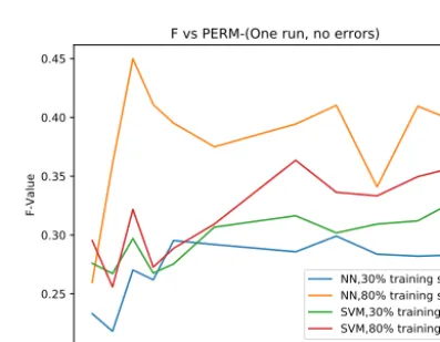
10. In-deed, thismodel could be used toshortlist 447 out ofthe 1584 forfurtherstudy,but417 ofthemare falselypredictedtohavea symmetryandworsestillthismodelmissesaquarteroftheactual CICYswithasymmetry.

PERMresultsaresummarizedinTable5andFig.6.Notethese resultsare notaveragedoverseveralrunsandare thusnoisy.We seethatfor80% ofthetrainingdataused(thesametrainingsizeas used forSMOTEruns) thatthe F-valuesareofthe order0.3–0.4. This is aslight improvementover SMOTE, butwe note from the PERM 100

,

000 resultsinTable5there isalimit tothe improve-mentpermutationscangive.

Identifyingtheexistence andtheformoffreelyactingdiscrete symmetries ona Calabi–Yau geometryis adifficult mathematical problem. It is therefore unsurprising that the machine learning algorithms also struggle when confronted with the challenge of findingararefeatureinthedataset.

5. Discussion

[image:7.612.31.285.296.503.2]

[image:8.612.100.509.63.394.2] [image:8.612.336.535.439.594.2]

Fig. 5.ROCand F-curvesgeneratedforbothSVMandneuralnetworkforseveralSMOTEvaluesbysweepingthresholdsandaveragingover100 differentrandomcross validationsplits.Herewepresentresultsafterthemodelshavebeentrainedon80% ofthe trainingdata.Shadingrepresentspossiblevaluestowithinonestandarddeviation ofmeasurements.

Table 5

F-values obtainedfordifferentamountsofPERMSforonerun.Dashescorrespond toexperimentswhichcouldn’tberunduetomemoryerrors.

30% Training Data 80% Training Data PERM NN F-Value SVM F-Value NN F-Value SVM F-Value

100000 0.2857 – 0.3453 –

10000 0.3034 0.2989 0.3488 – 2000 0.2831 0.3306 0.3956 0.3585 1800 0.2820 0.3120 0.4096 0.3486 1600 0.2837 0.3093 0.3409 0.3333 1400 0.2881 0.3018 0.4103 0.3364 1200 0.2857 0.3164 0.3944 0.3636 800 0.2919 0.3067 0.3750 0.3093 600 0.2953 0.2754 0.3951 0.2887 500 0.2619 0.2676 0.4110 0.2727 400 0.2702 0.2970 0.4500 0.3218 300 0.2181 0.2672 0.3607 0.2558 200 0.2331 0.2759 0.2597 0.2954

theSVMtoperformbetterforsucharchitectures.Theneural net-workhowever,was better atpredicting Hodge numbers thanthe SVM.Heretheneuralnetworkarchitecture isfarfromtrivial, and its success over SVMs is likely dueto its greater flexibility with non-linear data. To benchmark the performance of each model weuse crossvalidationandtake a varietyof statisticalmeasures whereappropriate,includingaccuracy,Wilsonconfidenceinterval, F-values, andtheareaunderthe receivingoperatorcharacteristic (ROC)curve(AUC).Errors wereobtainedbyaveragingoveralarge sample of cross validation splits and taking standard deviations. Models are optimised by maximising the appropriate statistical measure.Thisisachievedeitherbyvaryingthemodelbyhandor

Fig. 6.Plot of permutationF-values up to PERM 2000.

by implementing a genetic algorithm. Remarkable accuraciescan be achieved, even when, forinstance,trying to predict the exact valuesofHodgenumbers.

[image:8.612.42.294.470.606.2]

72 K. Bull et al. / Physics Letters B 785 (2018) 65–72

Acknowledgements

ThispaperisbasedontheMastersofPhysicsprojectofKBwith YHH,bothofwhomwouldliketothanktheRudolfPeierlsCentre forTheoreticalPhysics,UniversityofOxfordfortheprovisionof re-sources.YHHwouldalsoliketothanktheScienceandTechnology FacilitiesCouncil,UK,forgrantST/J00037X/1,theChineseMinistry ofEducation,foraChang-JiangChairProfessorshipatNanKai Uni-versityandtheCityofTian-JinforaQian–RenScholarship,aswell asMertonCollege,UniversityofOxford,forher enduringsupport. VJissupported by theSouthAfricanResearchChairs Initiative of theDST/NRFgrantNo.78554. HethanksTsinghuaUniversity, Bei-jing,forgenerous hospitalityduring thecompletion ofthiswork. We thank participants at the “Tsinghua Workshop on Machine LearninginGeometryandPhysics2018”forcomments.CMwould liketothankGoogle DeepMind forfacilitating helpfuldiscussions withitsvariousmembers.

References

[1]Y.-H.He,Deep-learningthelandscape,arXivpreprint,arXiv:1706.02714. [2] Y.-H. He, Machine-learning the string landscape, Phys. Lett. B 774(2017)

564–568,https://doi.org/10.1016/j.physletb.2017.10.024.

[3]D.Krefl, R.-K.Seong,MachinelearningofCalabi–Yauvolumes, Phys.Rev.D 96 (6)(2017)066014.

[4]Y.-N.Wang,Z. Zhang,Learning non-higgsable gaugegroups in4df-theory, arXivpreprint,arXiv:1804.07296.

[5]J.Carifio,J.Halverson,D.Krioukov,B.D.Nelson,Machinelearninginthestring landscape,J.HighEnergyPhys.2017 (9)(2017)157.

[6]F.Ruehle,Evolvingneuralnetworkswithgeneticalgorithmstostudythestring landscape,J.HighEnergyPhys.2017 (8)(2017)38.

[7]S. Abel,J.Rizos, Genetic algorithmsand the searchfor viablestring vacua, J. HighEnergyPhys.2014 (8)(2014)10.

[8]J. Carifio,W.J. Cunningham,J.Halverson, D. Krioukov,C. Long, B.D.Nelson, Vacuum selectionfrom cosmologyonnetworks ofstring geometries,arXiv: 1711.06685.

[9]P.Green,T.Hübsch,Calabi–Yaumanifoldsascompleteintersectionsinproducts ofcomplexprojectivespaces,Commun.Math.Phys.109 (1)(1987)99–108. [10]P.Candelas,A.M.Dale,C.Lütken,R.Schimmrigk,CompleteintersectionCalabi–

Yaumanifolds,Nucl.Phys.B298 (3)(1988)493–525.

[11] P.Candelas,R.Davies,NewCalabi–YaumanifoldswithsmallHodgenumbers, Fortschr. Phys. 58 (2010) 383–466, https://doi.org/10.1002/prop.200900105, arXiv:0809.4681.

[12]V.Braun, Onfree quotients ofcompleteintersection Calabi–Yau manifolds, J. HighEnergyPhys.04(2011)005.

[13]A.Lukas,C.Mishra,DiscretesymmetriesofcompleteintersectionCalabi–Yau manifolds,arXivpreprint,arXiv:1708.08943.

[14]P. Candelas, C. Mishra, Highly symmetric quintic quotients, Fortschr. Phys. 66 (4)(2018)1800017.

[15] P.Candelas,A.Constantin,CompletingthewebofZ3–quotientsofcomplete

intersectionCalabi–Yaumanifolds,Fortschr.Phys.60(2012)345–369,https:// doi.org/10.1002/prop.201200044,arXiv:1010.1878.

[16]P.Candelas,A.Constantin,C.Mishra,HodgenumbersforCICYswith symme-triesoforderdivisibleby4,Fortschr.Phys.64 (6–7)(2016)463–509. [17]A.Constantin,J.Gray,A.Lukas,HodgenumbersforallCICYquotients,J.High

EnergyPhys.2017 (1)(2017)1.

[18]P.Candelas,A.Constantin,C.Mishra,Calabi–Yauthreefoldswithsmallhodge numbers,arXivpreprint,arXiv:1602.06303.

[19] L.B. Anderson,Y.-H.He, A.Lukas,Heteroticcompactification,analgorithmic approach,J.HighEnergyPhys.0707(2007)049,https://doi.org/10.1088/1126 -6708/2007/07/049,arXiv:hep-th/0702210.

[20] L.B.Anderson,Y.-H.He,A.Lukas,Monadbundlesinheteroticstring compact-ifications,J.HighEnergyPhys.0807(2008)104,https://doi.org/10.1088/1126 -6708/2008/07/104,arXiv:0805.2875.

[21]L.B.Anderson,J.Gray,Y.-H.He,A.Lukas,Exploringpositivemonadbundlesand anewheteroticstandardmodel,J.HighEnergyPhys.2010 (2)(2010)1. [22] L.B.Anderson,J.Gray,A.Lukas,E.Palti,Twohundredheteroticstandardmodels

onsmoothCalabi–Yauthreefolds,Phys.Rev.D84(2011)106005,https://doi. org/10.1103/PhysRevD.84.106005,arXiv:1106.4804.

[23] L.B.Anderson,J.Gray,A.Lukas,E.Palti,Heteroticlinebundlestandard mod-els,J.HighEnergyPhys.1206(2012)113,https://doi.org/10.1007/JHEP06(2012) 113,arXiv:1202.1757.

[24] A.Lukas,L.Anderson,J.Gray,Y.-H.He,S.-J.L.Lee,CICYlistincludingHodge numbersandfreely-actingdiscretesymmetries,Dataavailableonlineathttp:// www-thphys.physics.ox.ac.uk/projects/CalabiYau/cicylist/index.html,2007. [25]L.B.Anderson,X.Gao,J.Gray,S.-J.Lee,FibrationsinCICYthreefolds,J.High

EnergyPhys.2017 (10)(2017)77.

[26] L.Anderson,X.Gao,J.Gray,S.J.Lee,ThefavorableCICYlistanditsfibrations, http://www1.phys.vt.edu/cicydata/,2017.

[27]T.Hubsch, Calabi–Yau Manifolds, aBestiaryfor Physicists, WorldScientific, 1992.

[28]N.V.Chawla,K.W.Bowyer,L.O.Hall,W.P.Kegelmeyer,Smote:synthetic minor-ityover-samplingtechnique,J.Artif.Intell.Res.16(2002).

[29]M.Kreuzer,H.Skarke, Completeclassificationofreflexivepolyhedrain four-dimensions,Adv.Theor.Math.Phys.4(2002)1209–1230.

[30] R.Altman, J. Gray, Y.-H.He, V.Jejjala,B.D. Nelson, ACalabi–Yau database: threefoldsconstructedfromtheKreuzer–Skarkelist,J.HighEnergyPhys.02 (2015)158,https://doi.org/10.1007/JHEP02(2015)158,arXiv:1411.1418. [31]J.Gray,A.S.Haupt,A.Lukas,AllcompleteintersectionCalabi–Yaufour-folds,