Situated Planning for Execution Under Temporal Constraints
Michael Cashmore, Andrew Coles
King’s College LondonBence Cserna
University of New HampshireErez Karpas
Technion — Israel Institute of Technology
Daniele Magazzeni
King’s College LondonWheeler Ruml
University of New HampshireAbstract
One of the original motivations for domain-independent plan-ning was to generate plans that would then be executed in the environment. However, most existing planners ignore the pas-sage of time during planning. While this can work well when absolute time does not play a role, this approach can lead to plans failing when there are external timing constraints, such as deadlines. In this paper, we describe a new approach for time-sensitive temporal planning. Our planner is aware of the fact that plan execution will start only once planning finishes, and incorporates this information into its decision making, in order to focus the search on branches that are more likely to lead to plans that will be feasible when the planner finishes.
Introduction
One of the original motivations for domain-independent planning was for controlling robots performing complex tasks (Fikes and Nilsson 1971). The typical approach to con-trolling robots using a planner is to call the planner to gen-erate a plan which solves the problem, and then execute that plan in the environment. This approach works well if the plan remains applicable regardless of when it is executed. However, if there are external timing constraints, such as deadlines which must be met, things become more complex. This is because we must take into account theplanning time. For example, in the Robocup Logistics League (RCLL) challenge (Niemueller, Lakemeyer, and Ferrein 2015), a team of robots must move workpieces between different ma-chines that perform some operations on them, and fulfill some order with a deadline. This calls for using temporal planning, because we would like all robots to work in par-allel, and actions have different durations. The typical ap-proach would have the planner come up with a plan which would work had it been executed at time 0, and then execute this plan when the planner completes. Obviously, this might lead to missing the deadline, and thus, plan failure.
One simple approach to handling this problem is to use some estimate on how long planning will take, and adapt all the deadlines assuming plan execution would start when the planner finishes. While using an upper bound on planning time will eliminate the problem of plans failing, it might lead to the planner not finding a feasible plan to begin with. On the other hand, using too low an estimate could still lead to plans failing, as discussed above.
In this paper, we describe a new approach for situated temporal planning. Our planner is aware of the fact that plan execution will start once planning finishes, and incorporates this information into the internal data structure for temporal reasoning used by the planner, together with estimates of re-maining planning time. This helps our planner prune partial plans which are likely to lead to the planner finishing plan-ning too late for the plans to be of use, and focus on more promising branches of the search.
Our empirical evaluation demonstrates that this planner can handle temporal planning problems with absolute dead-lines much better than a naive baseline approach, in realis-tic settings where planning time counts, and the plan can only start executing once it is completed. To the best of our knowledge, this is the first temporal planner to explic-itly consider planning time, within the context of planning and execution. Thus, our planner is especially applicable to online planning for robotics, where a robot must find a plan to execute, but the world does not stop while the robot is planning.
Preliminaries
We consider propositional temporal planning problems with Timed Initial Literals (TIL) (Cresswell and Coddington 2003; Edelkamp and Hoffmann 2004). Such a planning problem Π is specified by a tuple Π = F, A, I, T, G, where:
• F is a set of Boolean propositions, which describe the state of the world.
• Ais a set of durative actions. Each actiona ∈ Ais de-scribed by:
– Minimum duration durmin(a) and maximum
dura-tion durmax(a), both in R0+ with durmin(a) ≤ durmax(a),
– Start condition cond(a), invariant condition cond↔(a), and end condition cond(a), all of which are subsets ofF, and
– Start effect eff(a) and end effect eff(a), both of
which specify which propositions in F become true (add effects), and which become false (delete effects). • I⊆Fis the initial state, specifying exactly which
• T is a set of timed initial literals (TIL). Each TILl ∈ T consists of a timetime(l) and a literallit(l), which specifies which proposition inF becomes true (or false) at timetime(l).
• G⊆F specifies the goal, that is, which propositions we want to be true at the end of plan execution.
A solution to a temporal planning problem is a schedule
σ, which is a sequence of triplesa, t, d, wherea ∈ Ais an action,t∈R0+is the time when actionais started, and
d∈[durmin(a),durmax(a)]is the duration chosen fora. A
schedule can be seen as a set of instantaneoushappenings (Fox and Long 2003), which occur when an action starts, when an action ends, and when a timed initial literal is trig-gered. Specifically, for each triplea, t, din the schedule, we have actionastarting at timet(requiringcond(a)to
hold a small amount of timebefore timet, and applying the effectseff(a)right att), and ending at timet+d
(re-quiringcond(a)to holdbefore t+d, and applying the effectseff(a)at timet+d). For a TILlwe have the effect
specified bylit(l)triggered at timetime(l). Finally, in or-der for a schedule to be valid, we also require the invariant conditioncond↔(a)to hold over the open interval between tandt+d, and that the goalGholds at the state which holds after all happenings have occurred.
Related Work
Temporal planners have of course been used in on-line ap-plications before. For example, researchers at PARC built a special-purpose temporal planner for on-line manufactur-ing (Ruml et al. 2011). As in many temporal planners, each search node contains a Simple Temporal Network (STN) (Dechter, Meiri, and Pearl 1991) to represent the time points of events in the plan and constraints on when they can occur. To reflect the fact that actions cannot occur until planning has completed, the PARC planner includes a hard-coded es-timate of the required planning time, and every time point in the STN is constrained to occur at least that far after the time that planning started (Ruml et al. 2011, Figure 11). While this is a reasonable solution in a domain where the expected planning problems are all of similar difficulty, this approach can perform poorly in domains that include a wide variety of problems, as we will see below.
There has also been work on time-aware planning in the search community. Dionne, Thayer and Ruml (2011) present a so-called ‘contract algorithm’ called Deadline-Aware Search (DAS) that, given a deadline, attempts to re-turn the cheapest complete plan that it can find within that deadline. The main part of the algorithm works by estimat-ing the time that will be required to find a solution beneath each node in the open list, and pruning those for which this estimate exceeds the remaining search time. The estimate is the product of three quantities that are determined on-line: the time required to expand a node, expressed in seconds, an estimate on the number of search nodes remaining on the path to a goal beneath the given node, notatedd(n), and the average number of expansions required before a generated node is selected for expansion, called theexpansion delay. Although DAS was shown to surpass anytime algorithms on
combinatorial benchmarks, its ideas have never been imple-mented in a domain-independent planner.
Bugsy (Burns, Ruml, and Do 2013) is a search algorithm that attempts to minimize the user’s utility, which is repre-sented as a linear combination of planning time and plan cost. If plan cost is makespan, then the utility measures the ‘goal achievement time’, or the time from when the goal is presented to the planner, and planning starts, to when the plan finishes executing, and the goal is achieved by the agent. Bugsy is a best-first search algorithm, and relies on an estimate of remaining planning time similar to that of DAS in order to estimate the utility of each node it expands. While Bugsy is sensitive to its own planning time, it is not cog-nizant of external timed events such as deadlines, and does not prune nodes based on temporal information.
Related concepts in the search community include real-time search and anyreal-time search. In the real-real-time search setting, the planner must return within a prespecified time bound the next action for the agent to take. This differs from our setting, in which the planner must return a complete plan and the temporal constraints are fine-grained and can relate individual domain propositions to absolute times. In anytime search, a planner quickly finds a complete plan, and then uses additional computation time to improve it until either it is terminated by an external signal or an optimal solution is found. In our setting, the planner may not run indefinitely, but rather is expected to minimize the agent’s goal achieve-ment time. And while doing so, we demand that the planner recognize that time is passing and that it be responsive to timed events in the external world.
Encoding Planning and Execution Time
Many temporal planners (e.g., (Coles et al. 2009; 2012; 2010; Benton, Coles, and Coles 2012; Fern´andez-Gonz´alez, Karpas, and Williams 2015; 2017)) rely on an internal Sim-ple Temporal Network (STN) (Dechter, Meiri, and Pearl 1991) (or possibly a linear program or a convex optimiza-tion problem — but we will abuse terminology and call all of these the STN) to represent the temporal constraints between the set of thetime pointswhere actions start or end. Specif-ically, planners that support required concurrency (Cushing et al. 2007) tend to use this representation to support concur-rent execution of actions.When planning is done offline, the STN contains some time pointtES, which is the start of plan execution, and is assigned the value of 0. For convenience, we split each oc-currence of actionain the plan into two snap-actions:aand
we would have t(a)−t(b) ≥ , where is the mini-mum separation between two events that depend on each other (Fox and Long 2003). Or, if the start of c threatens the preconditions ofd, thent(c)−t(d) ≥ . Addition-ally, timed initial literals (TIL) (Edelkamp and Hoffmann 2004) are encoded into the STN by adding a time pointt(f)
for the occurrence of TILf, with the temporal constraint
t(f)−tES=time(f), wheretime(f)is the time at which
f occurs, as specified in the problem definition. These are then ordered with respect to the other steps in the plan by, again, adding sequencing constraints due to the causal rela-tions betweenlit(f)and the other steps in the plan.
In this paper, we focus on onlineplanning. We want to account for the fact that time passes during the planning process, and that, in fact, planning time and execution time are both the same. In order to do so, we modify the STN described above by adding two additional time points:tP S which is the time when planning started, and tnow which is the current time. We add the temporal constraint that
tnow −tP S equals the currently elapsed time in planning. The expression tES −tnow corresponds to the remaining planning time, which is, of course, unknown. We will dis-cuss this expression, and how to treat it, in the next sec-tion. Now, tP S = 0, while tES is unknown. Finally, be-cause TILs describe absolute time, we must modify the tem-poral constraints corresponding to TILs to usetP Sinstead of tES, i.e., the temporal constraint for TIL l would be t(l)−tP S = time(l), wheretime(l)is the time at which
lmust occur.
Time-Aware Planning
We have described a technique for encoding an STN which captures the fact that execution only starts after planning ends, and planning takes time. We now describe the impact this has on search within a temporal planner.
Forward Planning Search Space
We take as our basis the forward-search approach of the plannerOPTIC(Benton, Coles, and Coles 2012). Here, each search state comprises the plan π (of snap actions) that reaches that state; the propositions p ⊆ F that hold after
πwas executed from the initial state; and the Simple Tem-poral NetworkSTN(π)encoding the temporal constraints overπ.
When expanding a state inOPTIC, successors were gener-ated in one of three ways:
• By applying a start snap-action that is logically appli-cable: anya wherep cond(a);eff(a)would not break the invariant condition of an action that has started inπbut not yet ended; andcond↔would be satisfied once a has been applied. In this case, in the successor state,
π=π+ [a],pis updated according toeff(a)to yield
p, and a variablet(a)added toSTN(π). Sequence con-straints are imposed on this such that it follows any step inπthat met one ofcond(a); or whose effects refer to the same propositions aseff(a); or whose preconditions
(including invariant conditions) would be threatened by
eff(a)1.
• By applying anendsnap-action that is logically applica-ble – anyawhereahas started inπbut not yet ended;
p cond(a); and whose effects eff(a) would not
break the invariant ofany otheraction that has started in
πbut not yet ended. In this case, the successor state is up-dated in a way analogous to starting an action, with the additional STN constraint durmin(a) ≤ t(a)−ta ≤ durmax(a).
• By applying aTimed Initial Literallthat has not already occurred inπ. In this case,π =π+ [l],pis updated ac-cording tolit(l)to yield p, and a variable t(l)is added to STN(π). For the purposes of sequence constraints, this can be thought of as being a snap-action with no pre-conditions – it suffices to order it after steps inπwhose preconditions or effects refer tolit(l). To fix the time at which l occurs, an additional STN constraint is added:
t(l)−tPS = time(l)– while snap-actions are ordered only relative to other points in the plan, TILs must also occur a specific amount of time after time zero.
State expansion in this way generates candidate succes-sors that are logically feasible; to ensure they are also tem-porally feasible, only those whose STNs are consistent are kept. Using an all-pairs shortest path algorithm in the STN will both check consistency (with negative cycles corre-sponding to an inconsistent STN), and give us the earliest and latest possible time at which each snap-action could be applied. We denote thesetmin(x)andtmax(x)for each STN variablet(x). Typically, only the former of these is used – to mapπ to a scheduleσ, each start–end snap-action pair
a,a gives a triplea, tmin(a),(tmin(a)−tmin(a)). In other words, apply each action as soon as possible, with the shortest possible duration, thereby minimizing execution time.
Extending this approach to planning while aware of plan-ning and execution time requires a number of modifications, which we now step through.
No action can start before plan execution starts – be-cause execution cannot start until a plan has been produced. That is, for each a in the plan π, we add a constraint
tES ≤ t(a)to the STN, where tES is the time at which execution will start. We do not know thisa priori, but can at least saytnow ≤tESis the time since the planner started ex-ecuting. An STN for a plan produced during successor gen-eration will then be consistentiffit is not already too late to start executing the plan.
These additional constraints can be thought of as pushing the earliest actions in the plan to start after now; the effects of which are then propagated through the STN to appropri-ately delay the later actions, according to the sequence and duration constraints. If an otherwise-consistent STN is made inconsistent by these, then necessarily there must be a snap-actionxwheretmax(x)< tnow – i.e. we are past the latest point at whichxcould have been applied.
1
Planning time particularly matters in the presence of TILs – in the absence of these, we can start executing a plan when-ever we like by simply delaying the start of the first action. If TILs are present, though, these anchor the plan to having to fit around absolute time: with reference to state expan-sion, when a TIL is added to the plan, this fixes it to come after any earlier steps with which it would interfere, thereby constraining their maximum time.
Automatically applying past TILs – if we are now past the time at which a TIL has occurred, it is added toπbefore expanding the state.
More formally, immediately before expanding a stateS=
π, p,STN(π), the following TILs are applied: {l∈T |t(now)≥time(l)∧l ∈π}
If there are several such TILs, they are applied in as-cending order oftime(l). The mechanism for applying these TILs is identical to that inOPTIC: each is applied, to yield a successor stateS; and thenSreplacesS. By doing this be-fore expanding the state, we account for time having passed sinceS having been placed on the open list, and it being expanded – if in this time a TIL will have happened, S is updated accordingly, before expansion.
If this modification was not made, search would be free to branch over what step should next be added toπ. In the case where a TILlrepresents a deadline – by deleting a precon-dition on actions that must occur by a given time – search would be free to apply these actions, even though in real-ity it is too late. By forcing the application of past TILs, we avoid this behavior: all such actions would then become in-applicable.
Pruning states where it is too late to start their plan From the STN for a planπ, we can note the latest point at which that plan can start executing; and prune any states for which this time has already passed.
As noted earlier, to check if the STN for a state is con-sistent, we use an all-pairs shortest path algorithm. This in-cidentally yields the minimum and maximum time-stamps for each snap-action. For snap-actions that are ordered be-fore a TIL – which are fixed in time – these maximum time-stamps are finite. Moreover, because the plan is ex-panded in a strictly forward direction, the maximum times-tamps are monotonically decreasing: it is not possible to somehow order a new action before a plan step, in a way that reduces its maximum time-stamp. Thus, for each state
S =π, p,STN(π)we identify the start snap-action inπ
that has the earliest possible maximum time-stamp – this is the latest time at whichπcould feasibly be executed:
latest start(π) = min{tmax(a)|a ∈π}
Then, whenSis about to be expanded – after it was gener-ated, placed on the open list, and then removed – it is pruned iftnow >latest start(π).
Experiments
[image:4.612.337.540.51.192.2]To gain a concrete sense of the practical import of our tech-nique, we experimentally compared it to the baseline method
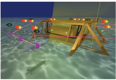
Figure 1: Screenshot of the underwater simulator, in which the AUV is inspecting the structure.
of prespecified planning times. We performed experiments in two types of domains: a realistic AUV simulation, and a set of IPC domains.
As a baseline against which to compare our time-aware planner, we usedOPTICin optimization mode, searching for the best plan within a varying fixed planning time ofT sec-onds. Time windows were considered to beT seconds ear-lier, to adjust the initial state to the start of execution time. Therefore, a TILloccurring at timetime(l)seconds, using a planning time ofTseconds, will occur at time(time(l)−T)
(at least0) in the plan.
AUVs
We demonstrate the approach in simulation with au-tonomous underwater vehicles (AUVs). We embed OPTIC and our planner into ROS, using ROSPlan (Cashmore et al. 2015), to control the AUV. The AUV is equipped with a manipulator and placed in an underwater structure, with the task to inspect certain areas and to ensure that valves are turned to correct angles. The valves can only be turned within certain time windows, outside of which the valve is blocked. If the valve cannot be turned to the correct angle within an early time window, then a later window can be used. We generated 41 missions with varying time windows. A screenshot of the simulation is shown in Figure 1
These missions normally form part of a larger, strategic mission, spread out over a number of seabed manifolds. The AUV moves between these manifolds in order to complete the missions. Due to the uncertainty in the environment, it is not known beforehand precisely what time the AUV will arrive at the manifold. Before beginning the task, the AUV must construct a new plan. Plans with shorter durations are considered to be of higher quality, as this eases the time con-straints on the remainder of the missions. We use this sce-nario to show that our approach allows the AUV to make use of earlier time windows, generating plans of higher quality.
Time Aware
OPTIC50 OPTIC100 OPTIC200
best quality 34 13 20 19
IPC quality 40.19 25.55 26.19 26.47
problems solved
[image:5.612.320.536.55.108.2]41 26 34 40
Table 1: Table comparing the number of problems solved, the number of plans of highest quality, and the IPC quality for each approach.
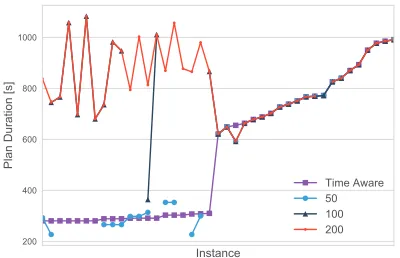
Figure 2: Plan durations per problem for each approach. The time-aware approach solves many problems using an earlier time window. OPTICusing a long planning time solves al-most every problem, but only using the later time windows. Other planning time bounds are less reliable.
also shows the number of best plans for each approach. This is the number of problems for which that approach produced the plan of highest quality between the four approaches (pos-sibly jointly). There it can be seen that although increasing the planning time allows for all problems to be solved, the quality is much poorer. The higher absolute number of best plans for the200second planning time is due to the greater number of problems solved. Finally, the table shows the IPC quality, calculated for all problems. These results demon-strate the choice between acting quickly, utilizing early time-windows, or producing plans reliably. Using the time-aware approach does both.
This can be seen more clearly in Figure 2. This figure compares the plan duration from each approach per prob-lem. UsingOPTIC200almost every problem is solved, at the longest possible plan duration – assuming planning takes 200 seconds forces the planner to have to use the later time windows. Other approaches may generate shorter plan dura-tions, but fail to solve many of the problems.
IPC Domains
In our IPC experiments, we tested all IPC-4 and IPC-5 do-mains that contain TILs: airport, pipesworld, satellite, truck, and UMTS. The UMTS domains and half of the airport instances were omitted as none of the planners completed
Time Aware OPTIC0.1 OPTIC1 OPTIC10
best quality 38 1 0 1
IPC quality 38 9.99 29.74 19.89
problems solved 38 10 30 21
Table 2: Table comparing the number of problems solved, the number of plans of highest quality, and the IPC quality for each approach
these. The planners were given a maximum of200sof CPU time and4GB of memory.
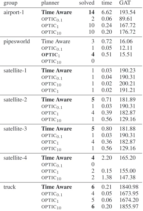
Table 2 presents results on the modified IPC domains. The fixed planning time planners were outperformed by the time-aware methods in every domain. Several instances were un-solvable by the former due to the fixed planning time con-straints. Table 3 shows the planners detailed performance in each relevant domain tested.
In addition to the fixed planning times that are showed in Table 2 and Table 3 we have tested50s,100s, and200s. The performance of the baseline approach with these planning times were lower than the time-aware method and the best presented baseline, thus these results were omitted.
Conclusions and Future Work
We have presented a domain-independent temporal planner that takes the interaction between the time spent on plan-ning and execution time into consideration. We have demon-strated empirically that this planner achieves much better re-sults in domains with absolute deadlines than our baseline approach. However, our work is merely the first step in ad-dressing this important topic. There remain many exciting avenues for future work.
For example, our planner only looks at the current par-tial plan, and uses a heuristic to “look” into the future. This heuristic is used to estimate the remaining search depth, but not to obtain more information about future actions and their effects on deadlines. In order to get a more informed view of future actions, and their effect on deadlines, we will ex-plore using temporal landmarks (Karpas et al. 2015). These landmarks could be encoded into the same STN of the par-tial plan, and thus we believe we will be able to achieve even better pruning of branches of the search tree which will not lead to a solution in time.
[image:5.612.67.267.199.328.2]group planner solved time GAT
airport-1 Time Aware 14 6.62 193.54
OPTIC0.1 2 0.06 89.61
OPTIC1 10 0.24 167.72
OPTIC10 10 0.20 176.72
pipesworld Time Aware 3 0.72 16.06
OPTIC0.1 1 0.05 12.11
OPTIC1 4 0.51 15.51
OPTIC10 0
satellite-1 Time Aware 1 0.03 190.23
OPTIC0.1 1 0.04 190.31
OPTIC10 1 0.02 200.21
OPTIC1 1 0.02 191.21
satellite-2 Time Aware 5 0.71 181.89
OPTIC0.1 1 0.03 190.31
OPTIC1 4 0.39 182.87
OPTIC10 1 0.56 129.16
satellite-3 Time Aware 5 0.80 181.88
OPTIC0.1 1 0.03 190.31
OPTIC1 4 0.36 182.87
OPTIC10 1 0.56 129.16
satellite-4 Time Aware 4 2.20 165.20
OPTIC0.1 0
OPTIC1 2 0.15 155.00
OPTIC10 2 1.38 147.38
truck Time Aware 6 0.21 1840.98
OPTIC0.1 4 0.05 1673.95
OPTIC1 5 0.06 1674.20
[image:6.612.54.294.54.408.2]OPTIC10 6 0.20 1855.97
Table 3: Table comparing the number of problems solved, the planning time, and the goal achievement time (GAT) grouped by IPC instance type. The planning time, and the GAT is the mean of all instances in the group solved by the planner.
planning time allocation into the search strategy.
One possible approach for this would be to treat the ex-pression tES −tnow as a variable, which we will denote byslack. We can then treat the STN as a mathematical op-timization problem, and maximize the slack. The slack for noden can serve as a proxy for the probability of finding a solution in time in the subtree rooted atn. Our metarea-soning algorithm could then choose the next node to expand based on both heuristic estimates and the slack.
Acknowledgements
This project has received funding from the European Union’s Horizon 2020 Research and Innovation programme under Grant Agreement No. 730086 (ERGO).
References
Benton, J.; Coles, A. J.; and Coles, A. 2012. Temporal planning with preferences and time-dependent continuous
costs. InProceedings of the 22nd International Conference on Automated Planning and Scheduling (ICAPS).
Burns, E.; Ruml, W.; and Do, M. B. 2013. Heuristic search when time matters. Journal of Artificial Intelligence Re-search47:697–740.
Cashmore, M.; Fox, M.; Long, D.; Magazzeni, D.; Ridder, B.; Carrera, A.; Palomeras, N.; Hurt´os, N.; and Carreras, M. 2015. Rosplan: Planning in the robot operating system. In Proceedings of the 25th International Conference on Auto-mated Planning and Scheduling (ICAPS), 333–341. Coles, A.; Fox, M.; Halsey, K.; Long, D.; and Smith, A. 2009. Managing concurrency in temporal planning us-ing planner-scheduler interaction. Artificial Intelligence 173(1):1–44.
Coles, A. J.; Coles, A.; Fox, M.; and Long, D. 2010. Forward-chaining partial-order planning. InProceedings of the 20th International Conference on Automated Planning and Scheduling (ICAPS), 42–49.
Coles, A. J.; Coles, A.; Fox, M.; and Long, D. 2012. COLIN: planning with continuous linear numeric change. Journal of Artificial Intelligence Research (JAIR)44:1–96.
Cresswell, S., and Coddington, A. 2003. Planning with timed literals and deadlines. InProceedings of 22nd Work-shop of the UK Planning and Scheduling Special Interest Group, 23–35.
Cushing, W.; Kambhampati, S.; Mausam; and Weld, D. S. 2007. When is temporal planning really temporal? In Pro-ceedings of the 20th International Joint Conference on Arti-ficial Intelligence (IJCAI), 1852–1859.
Dechter, R.; Meiri, I.; and Pearl, J. 1991. Temporal con-straint networks. Artificial Intelligence49(1-3):61–95. Dionne, A. J.; Thayer, J. T.; and Ruml, W. 2011. Deadline-aware search using on-line measures of behavior. In Pro-ceedings of the Symposium on Combinatorial Search (SoCS-11).
Edelkamp, S., and Hoffmann, J. 2004. PDDL2.2: The lan-guage for the classical part of the 4th international planning competition. Technical Report 195, University of Freiburg. Fern´andez-Gonz´alez, E.; Karpas, E.; and Williams, B. C. 2015. Mixed discrete-continuous heuristic generative plan-ning based on flow tubes. InProceedings of the 24th Inter-national Joint Conference on Artificial Intelligence (IJCAI), 1565–1572.
Fern´andez-Gonz´alez, E.; Karpas, E.; and Williams, B. C. 2017. Mixed discrete-continuous planning with convex op-timization. InProceedings of the 31st AAAI Conference on Artificial Intelligence, 4574–4580.
Fikes, R. E., and Nilsson, N. J. 1971. STRIPS: A new approach to the application of theorem proving to problem solving. InProceedings of the 2nd International Joint Con-ference on Artificial Intelligence (IJCAI), 608–620.
Pro-ceedings of the 25th International Conference on Automated Planning and Scheduling (ICAPS), 138–146.
Niemueller, T.; Lakemeyer, G.; and Ferrein, A. 2015. The RoboCup Logistics League as a Benchmark for Planning in Robotics. InWS on Planning and Robotics (PlanRob) at Int. Conf. on Aut. Planning and Scheduling (ICAPS).
Ruml, W.; Do, M. B.; Zhou, R.; and Fromherz, M. P. J. 2011. On-line planning and scheduling: An application to control-ling modular printers. Journal of Artificial Intelligence Re-search40:415–468.