A coupled bulk-surface model for cell polarisation

A COUPLED BULK-SURFACE MODEL FOR

CELL POLARISATION

Davide Cusseddu

, Leah Edelstein-Keshet

, John A. Mackenzie

,

St´

ephanie Portet

, Anotida Madzvamuse

Abstract: Several cellular activities, such as directed cell migration, are coordinated by an intricate network of biochemical reactions which lead to a polarised state of the cell, in which cellular symmetry is broken, causing the cell to have a well defined front and back. Recent work on balancing biological complexity with mathematical tractability resulted in the pro-posal and formulation of a famous minimal model for cell polarisation, known as the wave pinningmodel. In this study, we present a three-dimensional generalisation of this mathe-matical framework through the maturing theory of coupled bulk-surface semilinear partial differential equations in which protein compartmentalisation becomes natural. We show how a local perturbation over the surface can trigger propagating reactions, eventually stopped in a stable profile by the interplay with the bulk component. We describe the behavior of the model through asymptotic and local perturbation analysis, in which the role of the geometry is investigated. The bulk-surface finite element method is used to generate numer-ical simulations over simple and complex geometries, which confirm our analysis, showing pattern formation due to propagation and pinning dynamics. The generality of our mathe-matical and computational framework allows to study more complex biochemical reactions and biomechanical properties associated with cell polarisation in multi-dimensions.

Keywords: Cell polarisation; bulk-surface wave pinning model; coupled bulk-surface semi-linear partial differential equations; reaction-diffusion systems; bulk-surface finite elements; asymptotic and local perturbation theory

1

Introduction

Cell polarity is a complex process by which cells lose symmetry. However, its precise definition is still not very clear [16]. Polarity appears in single-cell organisms and multi-cell tissues. Many common basic polarisation mechanisms are shared and adapted by many different kinds of cells [40]. Roughly speaking, by breaking symmetry, cells define their front and rear and this process is characterised and driven by molecular chemical processes. Cell polarity is mediated and coordinated by a huge number of molecules and proteins and their interactions [9, 23]. The polarisation process, which can be caused by some external stimuli or can be spontaneous [3, 22], is necessary for many cellular activities, such as morphogenesis, and directed cell migration [30, 56]. Studies have identified the main directors of this phenomenon in the Rho family small guanosine triphosphate (GTP)-binding proteins (Rho GTPases). They behave like molecular switches, cycling between active (GTP-bound) and inactive forms (GDP-bound). Activation and inactivation are regulated by guanine nucleotide exchange factors (GEFs) and GTPase-activating proteins (GAPs). Moreover, the inactive Rho GTPases are sequestered in the cytosol by guanine nucleotide dissociation inhibitors (GDIs), that prevent the association of Rho GTPases with the plasma membrane [7, 24]. Among the Rho GTPase family, RhoA, Rac and Cdc42 are the most well known representatives in initiating the polarisation of migrating cells [13, 51, 53]. During cell migration, Rac and Cdc42 tend to concentrate their activities at the front, controlling the protrusive actin network, while RhoA is mostly active at the rear and regulates large focal adhesions

1_{Dept of Mathematics, School of Mathematical and Physical Sciences,University of Sussex, Brighton, UK}

E-mail contacts: [email protected](D. Cusseddu),[email protected](A. Madzvamuse)

and stress fibres [36, 42]. Microtubules and intermediate filaments are also involved in the process, for example binding the RhoA-effectors GEF-H1 and Solo [5, 17].

In recent years, Rho GTPases and cell polarisation have attracted the attention of many modellers [20, 47]. Mar´ee et al. [35] were able to simulate polarisation on a two-dimensional domain, in which the crosstalk between RhoA, Rac and Cdc42 in their active and inactive forms could generate the expected patterns. However, despite the fact that good computational results were obtained, a rigorous mathematical analysis of the biochemical system comprising six partial differential equations (PDEs), remained out of reach [11], until two years later, when Moriet al. [37] proposed a significant mathematical simplification of this modelling framework for cell polarisation, which became very popular and can be considered as the starting point of our study. The work in [37] focused on a conceptual minimal model of a single Rho GTPase and its switch between active and inactive forms, in which activation was supported by a positive feedback of the active GTPase in its own activation (see Figure 1 for a schematic representation). Their model consisted of the following pair

Figure 1: The minimal GTPase circuit with positive feedback for the activation ([37, 2]). Active GTPase is bounded to the membrane, while inactive GTPase moves in the cytosol.

of reaction-diffusion equations posed on a one dimensional domain

∂a ∂t =Da

∂2_a

∂2_x+f(a, b) x∈(0, L), t >0, (1)

∂b ∂t =Db

∂2_b

∂2_x−f(a, b) x∈(0, L), t >0, (2)

with

f(a, b) =k0+

γa2 K2_+a2

b−βa, (3)

and boundary conditions

∂a ∂x =

∂b

∂x = 0 x= 0, L, t >0, (4)

where a(x, t) and b(x, t) denote the active and inactive forms, respectively. Here, k0 represents the basal rate of activation and β is the rate of inactivation. The maximal rate for the positive feedback is indicated byγ andK is the parameter representing the quantity of aneeded to achieve a feedback-induced activation rate of γ/2 in the reaction.

The mathematical model was based on three key properties: (1) a large difference in diffusivities between active and inactive forms (Da/Db1); (2) conservation in time of the total mass

RL

0 (a+

b)dx; and (3) bistability in the reaction term f(a, b) with respect to a. Bistable reaction-diffusion equations are known to produce travelling waves for certain initial conditions [15]. In this work, [37], a local narrow peak of active GTPase was able to generate a travelling wave of active GTPase which is eventually stopped due to the interplay with the inactive GTPase, where conservation of total mass and fast cytosolic diffusion were key ingredients. An asymptotic analysis of the model, known as wave pinning (WP) phenomena, was later carried out in [38].

underlying mechanisms, not necessarily based on wave pinning. Some of them, however, share common features, for example positive feedback is still the key to achieve cell polarity in the work by Altschuler et al. [2], in which one ordinary and partial differential equation (ODE-PDE) system and one stochastic model are proposed for the interactions between an active and inactive GTPase component. Reaction-diffusion systems have also been used by Otsuji et al. [43]. They derive conceptual models of two components based on mass conservation and difference in diffusivity, which they show to be fundamental properties to achieve polarisation. In addition, Goryachev and Pokhilko [21] proposed a reaction-diffusion model for Cdc42 clustering in budding yeast, which was based on the Turing pattern formation mechanism. In [11, 28] some of these models are described and compared.

An important biological aspect of cell polarisation is the compartmentalisation of the membrane-bound and cytosolic proteins, which has inspired several works: Novaket al. presented a computa-tional approach for three-dimensional modelling of Rac proteins cycling between cell membrane and cytosol, using reaction diffusion equations [41]. In a more recent paper, [59], a one-dimensional model for Cdc42 and its GEFs in budding yeast is proposed. The cytosolic components purely diffuse over the line domain while slow membrane diffusion motivates the use of ordinary differential equations (ODEs) to model the membrane-bound species at the two ends. Interactions between the two occur through the flux conditions of the cytosolic components and the ODE reactions. A three-dimensional bulk-surface model showing Turing pattern formation is proposed in [49]. The GDI-bound inactive GTPase diffuses freely in the cell interior (the bulk) and, through an appropriate coupling boundary conditions, it binds to the cell membrane (surface of the domain), on which, its membrane-bound counterpart interacts with the active form. Both species were modelled by reaction-diffusion equa-tions. Another three-dimensional bulk-surface model is also proposed in [55]. This model is more detailed as all the three GTPases Cdc42, Rac, RhoA (in the cytosolic, membrane-bound active and membrane-bound inactive forms) and phosphatidylinositols (PIPs) are taken into account. The model results in a system of twelve reaction-diffusion equations.

The wave pinning model has seen its bulk-surface extension in two works [19, 46] and very recently in [8]. The first one by Ramirez et al. [46] adapts the WP model to GTPases in dendritic spines in neurons. The cytosolic GTPase is assumed spatially homogeneous, while the membrane-bound active form is subject to a surface reaction-diffusion equation. The interesting result is that the pinning mechanism can be induced only by the geometry of the domain: the smaller the neck of the spine, the easier is the confinement of the active GTPase. Confinement is also facilitated by higher diffusion, which however is in contrast with other models for cell polarisation based on slow membrane diffusivity. The second work, by Gieseet al. [19], presents a natural extension of the wave pinning model in the bulk-surface setting (see the following equations (5)-(8)), where the molecular interactions between the bulk and surface chemical components are mediated through an appropriate coupling boundary condition on the surface. In their work they investigate the role of shape, internal organelles and inhomogeneities in polarisation processes. Diegmilleret al. [8] have recently presented a three-dimensional analysis of the steady state of the wave pinning model in the bulk-surface setting on a sphere. They were able to show pattern formation in the surface component, after having shown analytically that spatial variation of the bulk component is negligible.

Inspired by these previous works, we study the extension of the wave pinning model in more general three-dimensional stationary convex and non-convex domains. Indeed in the work by [46] the geometry naturally reduces the model to a single one-dimensional reaction-diffusion equation and the cytosolic component is assumed constant, while [19] is an entirely two-dimensional work. Finally the work by Diegmilleret al. [8] reveals very important insights, however it is restricted to a sphere. The novelty of our work lies in that we mathematically quantify the role of the three-dimensional geometry in the wave pinning process, yielding new insights into this minimal model for wave pinning. For simplicity throughout the paper, we will refer to the reformulated WP model as the bulk-surface wave pinning (BSWP) model.

We present new three-dimensional results on regular and irregular geometries, exhibiting the wave pinning process on complex geometries. A key part of our study involves the numerical simulation of the BSWP model in three-dimensional geometries using a recently developed bulk-surface finite element method (BS-FEM) [10, 12, 31, 32, 33, 34]. This numerical framework allows to compute the solutions of the BSWP model on complex convex and non-convex geometries.

throughout this paper we confirm previous works based on the wave pinning model (1)-(3) and show analogies with our results. For example, we show the evolution of the solutions of the model at very large times which display interesting spatial effects. Our results reveal that certain geometries induce a metastable behavior of the model, in which the apparently stable active patch undergoes a very slow shifting on the surface towards more rounded areas of the domain. This was also shown in previous published results for the two-dimensional wave pinning model presented by [57]. In addi-tion, the BSWP model shows competition between active regions, as recently shown in the classical WP model [6]. We also show how the geometry of the domain plays a crucial role in the pattern formation for the special case of spatial homogeneous initial conditions. This was interestingly re-ported in the two-dimensional case by Giese et al. in [19]. Hence, our work through mathematical and numerical analysis, aims to extend the current knowledge of the wave pinning model to real-istic three-dimensional settings and to provide a satisfactory understanding of the influence of the geometry, showing the role that cell shape plays in the polarisation mechanism.

The structure of this work is therefore as follows: In Section 2 we describe the model and its parameters as well as discussing its fundamental properties. The polarisation mechanism of the BSWP model is explained in Section 3 by an asymptotic analysis on a simple geometry. In Section 4 we present the parameter regions for bistability and polarisation. Analysis of the steady states for the well-mixed system provide a bistability region, whereas spatial effects were studied using the local perturbation analysis (LPA) [25, 27]. This latter tool is able to identify parameter spaces in which a local and narrow perturbation of the spatially homogeneous slow-diffusing component can generate spatial effects on the system. In our work we present a novel application of the LPA in a bulk-surface setting, which provides a natural way to investigate the effect of the ratio between surface area and bulk volume on the system. In Section 5 we present the bulk-surface finite element method (BS-FEM) [31, 33], used to simulate the model on various geometries. Numerical results are then presented in Section 6 to confirm and validate theoretical findings. A summary of the main results and a discussion follow in Section 7, with suggestions on future extensions and applications of the BSWP model.

(a) (b)

Figure 2: (a) A three-dimensional domain Ω representing the cell. (b) Activation of the bulk species occurs through the boundary conditions and propagates over the surface Γ of the domain.

2

The bulk-surface wave pinning model

Param. Value/Units Description

a molµm−2 _{concentration of active GTPase}

b molµm−3 _{concentration of inactive GTPase}

Da 0.1µm2s−1 diffusion coefficient ofa

Db 10µm2s−1 diffusion coefficient ofb

k0 0.067s−1 basal activation rate

β 1 s−1 _{deactivation rate}

γ 1 s−1 _{feedback activation rate}

K 1 molµm−2 saturation parameter

n 2 Hill coefficient

ω µm volume to surface ratio membrane binding parameter

Table 1: Parameters used in the bulk-surface model; the diffusion coefficients are taken as in [44], and the kinetic parameter values as in [37].

For model consistency we need to require our solutions to be smooth enough, so we look forclassical

solutionsa∈C(Γ×[0, T])∩C2,1(Γ×(0, T]) andb∈C(Ω×[0, T])∩C2,1(Ω×(0, T])∩C1,0_{(Ω×(0, T]),} whereCk,hindicates the set of functionsktimes differentiable in space andhtimes in time. We will assume pure diffusion for the cytosolic form and impose Robin-type boundary conditions on Γ, which take into account the switching between active and inactive species. From conservation principles we get

∂b

∂t =Db∆b, x∈Ω, t∈(0, T], (5) −Db(n· ∇b) =f(a, b), x∈Γ, t∈(0, T], (6)

where Db represents the diffusion coefficient,nis the outward unit vector to Ω and f is a function which depends on bothaandband represents the variation of the bulk variable bdue to activation and inactivation of the GTPase on the cell membrane. One key property of the model is that the reactions for the bulk species are incorporated into the boundary condition, while no reactions occur inside the cell. We use a relatively simple nonlinear reaction function f(a, b), the same as in [37]. Nonlinearity is achieved through a Hill function, commonly used in biochemistry to represent what is called acooperative binding [39]. One can work with a generalised function of (3) given by

f(a, b) =ωk0+

γan Kn_+an

b−βa, (7)

where the Hill coefficient n = 2 is sufficient to achieve bistability [37, 38], It must be noted that other choices for n have been presented [8, 26]. Following [48] we define ω := |Ω|/|Γ| as the ratio between bulk volume and surface area; it characterises the geometric effects in the reaction function and can be seen as a parameter describing the proteinbinding to the cell membrane. The length unit dimension of ω is needed to reduce the dimensionality of the bulk protein to the two-dimensional surface, where activation occurs. For a fixed volume,ωis maximal when Ω is spherical, so activation is enhanced in resting cells which generally have, at least in two-dimensions, a rounded shape [29].

The spatio-temporal dynamics of the membrane-bound active form aon the cell membrane are described by the following surface reaction-diffusion equation

∂a

∂t =Da∆Γa+f(a, b), x∈Γ, t∈(0, T], (8)

whereDa is the diffusion coefficient and ∆Γ is the Laplace-Beltrami operator, which generalises the Laplacian over manifolds [10] and it is here used to describe lateral diffusion of membrane proteins. Since we are considering a closed system in whichaandbare different forms of the same component, it makes sense to link entirely the reaction in a with the boundary condition for b, meaning that there is full inter-conversion between the two forms. Therefore the reaction in the equation for a

It should be noted that the well-posedness and the global existence of solutions for the general bulk-surface reaction-diffusion system ofkbulk andmsurface variables was studied by Sharma and Morgan in [54]. Hence, the following theorem holds:

Theorem 2.1. The BSWP model (5)-(8) admits a unique and non-negative classical solutiona(t,x) andb(t,x) at any timet >0, for any suitable non-negative initial condition ain(x) andbin(x).

Proof. See [54] and in particular Corollary 3.4.

2.1

Fundamental properties of the BSWP model

We now briefly present some fundamental properties of the BSWP model (5)-(8) as follows.

1. Conservation of total species. Integrating (5) and (8) and applying the divergence theorem on a manifold with boundary condition (6) and the divergence theorem on manifolds without boundary, it is easy to prove the following.

Proposition 2.1. Letaandb be solutions of (5)-(8). Then

M(t) :=

Z

Ω

b(x, t) dx+

Z

Γ

a(x, t) ds=M0, ∀t≥0 (9)

for a certain fixed valueM0 ∈R, defined by the initial conditions: indeed, M0 represents the total amount of substancea+b in the cell.

2. Difference in diffusivities. As protein diffusion over the membrane is known to occur much slower than in the cytosol, we considerDaDb [44].

3. Bistability. The following proposition holds

Proposition 2.2. Consider a fixed value ofb, denoted b. Therefore, there exist two positive valuesb1andb2such that ifb∈(b1, b2), the functionf(a, b), as defined in (7), can have up to three zerosa1(b)< a2(b)< a3(b). In particular, when this occurs we have [38]

∂f

∂a(a1(b), b)<0, ∂f

∂a(a2(b), b)>0, ∂f

∂a(a3(b), b)<0. (10)

See also Figure 3 for a schematic representation. In particular, a necessary condition for bistability [38] is that

8k0< γ. (11)

This latter condition represents and highlights the important role of the feedback-induced activation rate in the model.

3

Asymptotic analysis on a disk

The basic mechanisms of the BSWP model (5)-(8) can be understood through an asymptotic analysis which is here presented in order to highlight the main steps of the spatio-temporal evolution of certain classes of initial conditions. Since the core of the analysis is based on the crucial difference of protein diffusivity between cell membrane and cytosol, a convenient setting to stress this relationship is the use of a nondimensional version of the model. Therefore, in this section we consider the following coupled system of bulk-surface reaction-diffusion equations, where diffusion on the surface is very slow relative to diffusion in the bulk

ε∂b

∂t = ∆b, x∈Ω, (12)

−(n· ∇b) =f (a, b), x∈Γ, (13)

ε∂a ∂t =ε

2_∆

with

f(a, b) :=

k0+

γa2

1 +a2

b−a, (15)

where aandb are now nondimensional quantities andε2 ₌ Da

Db is a small parameter. Details of the nondimensionalisation can be found in the Appendix.

Provided condition (11) is satisfied, forb within a certain range (b1, b2), the functionf(a, b) has three distinct and positive roots a1(b)< a2(b)< a3(b) and (10) is satisfied, i.e. a1(b) and a3(b) are stable steady states for the ODE corresponding to the equation (14) with zero diffusion. Bistable reaction-diffusion equations are known to produce travelling wave solutions [15] and this is a crucial aspect of the wave pinning mechanism. Figure 3 shows the zero level set ofz =f(a, b), which also represents the nullcline of the ordinary differential system.

b

1.8 2 2.2 2.4 2.6 2.8 3

a

0 0.5 1 1.5 2 2.5

a(b) : f(a(b),b)=0

a

1(b)

a₂(b) a

3(b)

Figure 3: The solutions (a, b) solving f(a, b) = 0 as defined in (15) with parameters k0 = 0.05 and

γ= 0.79.

We consider initial conditions of the following type

bin(x) =b0∈(b1, b2), x∈Ω, (16)

ain(x) =ag+ap(x), x∈Γ, (17)

where ag ∈0, a2(b0)andap is a continuous function over Γ such that if

Γp:=

x∈Γ : ap(x) +ag> a2(b0)

then

0<|Γp|

|Γ| 1 and

1

|Γ|

Z

Γp

ap dx1.

In biological terms, the above describe that initially the inactive cytosolic protein is homogeneously constant, while the initial concentration ofais less than the valuea2(b0) in most of its domain except for tiny regions in which its mass is negligible. In the simulations we have representedap with very narrow Gaussian functions.

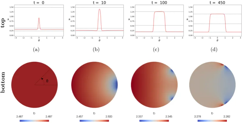
We consider a flat cell Ω = {(x, y) : x2_+y2 _{< r}2_{, r > 0} which, being a simple circular} domain, makes the exposition clearer. We are also interested in a single peak for a, which means Γp is connected, in other words,ain(x) =a2(b0) has two solutionsx. In our exposition we next show that the evolution ofais strongly characterised by different time scales with the development of well defined spatial patterns and formation of boundary layers in which the solution drastically passes from one “stable” state to the other. This corresponds to a sudden large variation of the gradient of

top

(a) (b) (c) (d)

b

ottom

Figure 4: Numerical solutions of the BSWP model (12)-(15) with ε2 _{= 0.001 on a disc at different} time steps. The parameter εplays a crucial role in sharpening the fronts of the solutiona[38] and smaller choices ofε result in a clearer effect of the BSWP mechanism. On the top row we plot the solutiona(red line) over the circle at different time steps, whereas the horizontal dashed lines indicate the three solutionsa1, a2, a3off a, b

= 0, whereb=_|Ω1_|R

Ωbdxanda1< a2< a3. On the bottom row we plot the solutionbinside the disk. It is important to note the scale values forb: at every time step,b is approximately spatially constant. (a) (top) A narrow Gaussian function is summed over a spatially homogeneous initial condition. In most of its domain ais initially smaller thana2, except for the Gaussian peak. We use the centre of the peak as reference for the polar coordinate system. (bottom) The initial condition forbis spatially homogeneous. (b) (top) Attraction ofatowards the valuesa1 anda3 is well visible: the peak grows towardsa3, while the rest of the solution tends to the lower valuea1. (bottom) Depletion ofb starts from the boundary of the disc at around θ = 0. (c) (top) At time t= 100aoverlaps a1 anda3 in most of the domain except in the two very small areas where the transition between the two states occurs very sharply. In addition, the peak of a

has visibly increased its width, as propagation has started. (bottom)bis depleted in correspondence of the sharp moving fronts of active GTPase. (d) The steady states for a andb. b has reached its critical value and there is no more source of GTPase available fora, which therefore is pinned in an almost piece-wise constant shape. Details of the numerical methods and tools used for the simulation will be given in Section 5.

through multiple temporal rescaling and matched asymptotic analysis. Our analysis is described in four steps (see also Figure 4) as outlined below, and it follows the asymptotic analysis done by Moriet al. [38] for the unidimensional model (1)-(3), which we have re-adapted to the BSWP model (5)-(8) thanks to the circular geometry.

(a) At the initial time, aevolves into a well defined profile with two fronts: over Γp it is attracted by a3(b), while on the rest of the domain it is attracted by a1(b). On the other hand, b is approximately spatially homogeneous. We study this evolution over the zoomed time scale

τ=t/ε.

(b) In the intermediate time scale t we observe the movement of the fronts in the a profile, in particular we are interested in the expansion of the high concentration peak. In order to achieve this, we need to show that

• The speed of the propagating fronts is strictly related to the sign of the function defined by

I(b) :=

Z a3(b)

a1(b)

• I(b) is an increasing function in (b1, b2) and there existsbc∈(b1, b2) such thatI(bc) = 0.

(c) The propagation ofacoincides with the depletion ofb, which is always approximately spatially homogeneous (note the color scale in Fig 4 bottom).

(d) Under particular conditions on the initial concentrations, the propagation stops before the whole boundary is activated. This occurs whenbhas decreased to its critical valuebc.

We are now in a position to discuss the steps (a)-(d) in more detail.

Step a)We first study the initial evolution of the system (12)-(15) by introducing the fast time scaleτ=t/ε. Temporal rescaling results in the following coupled bulk-surface system

∂b

∂τ = ∆b, x∈Ω,

∂a ∂τ =ε

2_∆

Γa+ f(a, b), x∈Γ,

−(n· ∇b) =f (a, b) x∈Γ.

Looking for solutions of the forma=a0+a1ε+a2ε2+· · · andb=b0+b1ε+a2ε2+· · · we find, at the leading order

∂b0

∂τ = ∆b0, x∈Ω,

∂a0

∂τ =f(a0, b0), x∈Γ, −n· ∇b0=f(a0, b0), x∈Γ.

The equation fora0is an ordinary differential equation and, at eachx, the solution will tend to the stable stationary pointa3(b) forx∈Γp ora1(b) elsewhere: at the end of this time scale we will have

∂a0

∂τ ≈0. This means that over Γ,f(a0, b0)≈0.

The equation for b0 is the heat equation with Neumann boundary conditions that will become approximately homogeneous at the end of the time scale. Thenb0(x, τ) will tend to reach a spatially homogeneous profile over the domain Ω.

Step b)In the intermediate time scalet, we again look for solutions of the forma=a0+a1ε+

a2ε2+· · · andb=b0+b1ε+a2ε2+· · ·. At the leading order we have

∆b0= 0, x∈Ω,

f(a0, b0) = 0, x∈Γ,

−n· ∇b0=f(a0, b0), x∈Γ.

We see that the flux condition is actually −n· ∇b0= 0, consistent with the Laplace equation in Ω.

b0(x, t) is now at equilibrium all over the domain. On the other hand,a0(x, t) remains at its low and high values, eithera1(b) ora3(b). This is valid far from the two front layers where the solution passes froma1 toa3and vice versa. Our goal is to see if these front layers move in time over the boundary Γ. We take advantage of the circular geometry of the domain and re-write the model (12)-(15) in polar coordinates

ε∂b ∂t =

∂2_b

∂ρ2+ 1

ρ ∂b ∂ρ +

1

ρ2

∂2_b

∂θ2, ρ∈(0, r), θ∈(−π, π],

ε∂a ∂t =

ε2

r2

∂2_a

∂θ2 +f(a, b), ρ=r, θ∈(−π, π],

−∂b

∂ρ =f(a, b), ρ=r, θ∈(−π, π],

at the centre of the boundary subset Γp, so that there exist a valueθ1< π such that Γp= (−θ1, θ1), see also Figure 4a (top and bottom).

The positions of the two fronts ofaare therefore initially defined by−θ1 andθ1 and our goal is to show that these positions can change in time subject to (12)-(15). We will consider θ1(t), which is initially small. We define the variable

ϕ1(t) :=

θ−θ1(t)

ε ,

such that

lim ε→0ϕ1=

(

+∞ ifθ > θ1

−∞ ifθ < θ1

and

lim

ϕ1→−∞a(ϕ1) =a3(b), ϕ1→lim+∞a(ϕ1) =a1(b),

i.e. the wave front connects the high and low plateau values ofa. We remark that for θ < 0 the situation reverses: the solution is close to a1(b) for values of θ < −θ1 and to a3(b) for θ > −θ1. More generally, the periodicity of the two-dimensional domain requires an even number of fronts in (−π, π], which was not necessary in previous works on the wave pinning mechanism. The equation

forain the new coordinate ˆa(ϕ1(t), t) =a

_θ−θ 1(t)

ε , t

is

εdˆa dt −θ

0

1(t)

∂ˆa ∂ϕ1

= 1

r2

∂2_aˆ

∂ϕ2 1

+f(ˆa, b), ϕ1∈(−∞,+∞).

The termθ₁0(t) in the left hand side of the above equation describes the speed of the front, which we want now to investigate. Using again asymptotic expansion ˆa=P_ˆa

iεiwe get, at the leading order

1

r2

∂2_ˆa 0

∂ϕ2 1

+θ0₁(t)∂ˆa0

∂ϕ1

+f(ˆa0, b) = 0, ϕ1∈(−∞,+∞).

Multiplying the above by ∂ˆa0

∂ϕ1 and integrating inϕ1∈(−∞,∞) leads to

1 2r2

Z +∞

−∞

∂ ∂ϕ1

∂ˆa0

∂ϕ1

2

dϕ1+θ10(t)

Z +∞

−∞

∂ˆa0

∂ϕ1

2

dϕ1+

Z +∞

−∞

f(ˆa0, b0)

∂aˆ0

∂ϕ1

dϕ1= 0.

The first integral is zero

1 2r2

Z +∞

−∞

∂ ∂ϕ1

_∂ˆa

0

∂ϕ1

2

dϕ1= 1 2r2

_∂ˆa

0

∂ϕ1

2

ϕ1=+∞

ϕ1=−∞

= 0,

since ˆa0 is constant at the limits ofϕ1. Applying a change of variables= ˆa0(ϕ1, t) the last integral can be written as

Z +∞

−∞

f(ˆa0,¯b0)

∂aˆ0

∂ϕ1

dϕ1=−

Z a3(¯b0)

a1(¯b0)

f(ξ,¯b0) dξ.

Hence, finally the following equality holds

θ0₁(t) =

Ra3(¯b0)

a1(¯b0) f(ξ,

¯

b0) dξ

R+∞ −∞

_∂ˆa 0

∂ϕ1 2

dϕ1

. (19)

AsR+∞ −∞

∂aˆ0

∂ϕ1 2

dϕ1>0, the previous equality gives us an important information about the speed of the front, which moves with the same sign of the function

I(b) =

Z a3(b)

a1(b)

Figure 5: The integral I(b) =Ra3(b)

a1(b) f(a, b)da withf defined in (15) and parameter values in Table

1. I(b) increases in [b1, b2] and has one zerobc ≈2.28, obtained by numerical estimation. The speed of the propagation of ais related to a decreasing of the bulk component and stops when b reaches the critical valuebc.

which is represented in Figure 5.

We remark thatI(b) is an increasing function, since

I0(b) =f(a3(b), b)a03(b)−f(a1(b), b)a01(b) +

Z a3(b)

a1(b)

∂f(a, b)

∂b da

=

Z a3(b)

a1(b)

k0+

γa2

1 +a2

da >0

given thata1(b)< a3(b) and the parameters k0 andγ are positive. The existence of a critical value

bcsuch thatI(bc) = 0 can be proven by showing that, for someε >0,I(b1+ε)<0 andI(b2−ε)>0, whereb1 andb2 are the extremal values for the existence of three zerosa(b) off(a, b). In fact when

b =b1 orb =b2 the functionf(a, b) has only two roots, i.e. between the roots it is either entirely negative or entirely positive. Ifb=b1−εorb=b2+εthen the integral is infinite. However asI(b) is an increasing function, by continuity it follows that I(b1+ε)<0 and I(b2−ε)>0. This shows the existence of the critical value bc and for (19) we know that for b > bc then aincreases its high concentration region.

Step c)We now prove that ifθ1increases, i.e. the high concentration peak foraexpands, then the quantitybdecreases all over the domain. Sincea1 anda3are not constant, in principle propagation of adoes not necessarily imply an increment of its overall amount (which, by conservation of total mass (9) would have implied depletion of b). Therefore, we start rewriting (9) at the leading order of the asymptotic expansion as

M0=

Z

Ω

b0 dx+

Z

Γ

a0ds+O(ε).

At the previous step we have seen thatb0 is spatially homogeneously distributed anda0 is approxi-mately a3(b0) if|θ|< θ1 ora1(b0) otherwise. Therefore we can rewrite the previous equation as

πr2b0(t) + 2θ1(t)r a3(b0) + 2r(π−θ1(t))a1(b0) +O(ε) =M0. (21)

Discarding terms O(ε) and differentiating (21) with respect tot results in

πr2b0₀(t) + 2rθ0₁(t)a3(b0) + 2rθ1(t)a03(b0)b00(t) + 2r(π−θ1(t))a01(b0)b00(t)−2rθ

0

from which, rearranging terms leads to

b0₀(t) =−2 a3(b0)−a1(b0)

πr2_{+ 2θ}

1(t)r a03(b0) + 2r(π−θ1(t))a01(b0)

θ0₁(t)r. (22)

We now prove that the denominator in (22) is positive. Let us differentiate with respect tobthe equationf(ai(b), b) = 0 fori= 1,3

0 = d

dbf(ai(b), b) =a

0

i(b)

∂f ∂a

_(a,b)=(a

i(b),b) +∂f

∂b

_(a,b)=(a

i(b),b)

. (23)

From which we get, if ∂f_∂a

(a,b)=(ai(b),b)

6

= 0, that

a0_i(b) =−

_∂f

∂a

_(a,b)=(a

i(b),b) −1

∂f ∂b

_(a,b)=(a

i(b),b)

. (24)

However, if the term in braces in (24) vanishes, then from (23), it needs to be that

∂f ∂b

_(a,b)=(a

i(b),b) = 0,

but this is not possible since

∂f ∂b =

k0+

γa2 1 +a2

>0, ∀a.

Hence, using (10) in (24), we conclude that

a0₁(b)>0, and a0₃(b)>0. (25)

From (25), it is now clear the positiveness of the denominator in (22), while the sign of the numerator of (22) is the opposite of the sign of θ₁0(t): if θ0₁(t)>0 then b0₀(t)<0 and vice-versa. This finally proves that the propagation of active GTPase aover the boundary is related to a decreasing of the bulk componentb.

Step d)In order to achieve polarisation, the propagation needs to stop, i.e. at a certain time ¯

t, θ01(¯t) = 0 and this happens whenb(t) reaches a minimum value bc. Therefore, ignoring terms of orderO(ε) we have

M0=πr2bc+ 2θ1(¯t)r a3(bc) + 2r(π−θ1(¯t))a1(bc).

We rewrite it in the form

M0=πr2bc+ 2rθ1(¯t) a3(bc)−a1(bc)

+ 2πr a1(bc).

Since we require 0< θ1< π then

M0< πr2bc+ 2πr a3(bc)−a1(bc)+ 2πr a1(bc) =πr2bc+ 2πr a3(bc)

and

M0> πr2bc+ 2πr a1(bc).

We therefore have found a condition on M0 equivalent to the classical wave pinning model [38]. To have pinning we need to take an initial value b0> bc anda0 such that

m1< M0< m2, (26)

4

Bistability and polarisation

In this section we are interested in mapping parameter regions for all possible different behaviors of the two- and three-dimensional BSWP model (5)-(8) in order to get some insights on the role of geometry. Indeed, depending on the parameters, the model is able to generate different responses, for example it supports spatial homogeneous solutions. We will start from this point, analysing the role of the reactions in the system. In a second step, we will use an approximated nonlinear analysis in order to identify the spatial responses of the BSWP model with respect to small perturbations of the boundary component from the spatially homogeneous state. We remark that the following analysis is basically independent of the spatial dimension.

4.1

Well mixed model

Integrating equation (5) in Ω and applying the divergence theorem with (6), we get

Z

Ω

∂b

∂t dx=−

Z

Γ

f(a, b) ds.

Since we want to consider spatial homogeneous solutions, this corresponds to

∂bg

∂t

Z

Ω

1 dx=−f(ag, bg)

Z

Γ 1 ds.

Finally, we will analyse the so-called well mixed system defined by

dag

dt =f(ag, bg), (27)

ωdbg

dt =−f(ag, bg), (28)

where we recall thatω=|Ω|/|Γ|denotes a parameter describing the geometry of the domain. Given that ωhas unit length makes the above system unit dimensionally consistent (see also Table 1). We note that the following quantity is conserved

ag(t)

ω +bg(t) = ag(0)

ω +bg(0),

which can be interpreted as a scaled total concentration. Indeed, it follows from (9) that

M0=

Z

Γ

a(x, t) ds+

Z

Ω

b(x, t) dx=|Γ|ag(t) +|Ω|bg(t) =|Ω|

_ag(t)

ω +bg(t)

.

The analysis of (27)-(28) reduces to the single equation

dag dt =f

ag, m0−

ag

ω

, (29)

where m0 := M_|Ω0_|. From the study of the steady states, f ag, m0− ag

ω

= 0 is a third degree polynomial in ag and, by the Descartes’ rule of signs, it can be shown that it has either one or three positive real roots. Therefore, from the negativity of the leading order coefficient, it follows that there exists either a single stable steady state or 3 steady states where the outer two are stable. Bistability corresponds to the co-existence of high and low GTPase activities at the cell membrane. When only a single steady state is possible, then the well mixed model admits only one response between low and high activities.

4.2

Local perturbation analysis

Local perturbation analysis (LPA) is a convenient tool that can be very useful in understanding how a local perturbation might affect some classes of reaction-diffusion systems with fast and slow components. We refer the interested reader to [25, 26, 27] for more details and the LPA. The basic idea is the following: let system (5)-(8) possess a spatially homogeneous profile (bg(t), ag(t)) and apply a narrow and well localised perturbation to the slow-diffusive componenta, such as defined by equation (17). Based on the fact that we have a fast and a slow variable (Db>> Da) we consider the limits Db → ∞ andDa →0. Therefore b maintains a global spatial uniform profile bG(t). On the other handa(x, t) has a global spatial uniform profileagin most of the cell membrane, except in the narrow area where the perturbation ap is applied. Considering the limitDa →0, the perturbation

apdoes not influence through diffusion the baseline levelag and, given its small mass, it does neither substantially influenceb. In these terms it is possible to considerap(t) andag(t) as different entities to obtain the following ODE system

dap

dt =f(ap, bg), (30)

dag

dt =f(ag, bg), (31)

ωdbg

dt =−f(ag, bg). (32)

It can be easily shown using conservation that the above system can be reduced to the following system

dap dt =f

ap, m0−

ag

ω

, (33)

dag dt =f

ag, m0−

ag

ω

. (34)

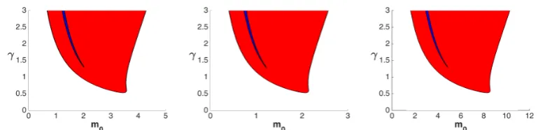
The above ODE system indicates that steady states forap might differ from the steady states forag. Indeed, we interpret this case as the polarisation response: the perturbation has affected the system and two states on the boundary are simultaneously present, with a localised high activity and low activity elsewhere. Using this analysis and numerical calculations, we obtain the polarisation region in the parameter planem0−γ, which is shown in red and blue color in Figure 6.

We have calculated the bistability and the polarisation regions for different values ofω, obtaining qualitatively identical results. However, the regions increase their sizes with decreasing ω. For the three-dimensional case, for a given volume |Ω|, maxΓω =r/3 where r is the radius of the sphere enclosing that volume. Therefore, having a fixed volume, the more the surface increases, the smaller

ω becomes. This is an interesting result which suggests that changes in shapes and increases in the cell surface relative to its volume enhance the possibility of achieving polarisation. Indeed a key feature of cell migration is the change in cell shape [50].

In [26] the same analysis was done for the model (1)-(3) whereaand bare defined on the same unidimensional spatial domain. They derive a well mixed and LPA system which is a special case of our models (28)-(27) and (30)-(32) whenω= 1. They initially use a sharp switch approximation for the reaction (7) (passing to the limit as n→ ∞) in order to be able to calculate the steady states analytically. Then they numerically calculate the bistability and polarisation regions for (7) with

n= 4. Our results, whenn= 2, are totally in line with their work and suggests that the bulk-surface framework maintains and extends the features of the original wave pinning model (1)-(2).

5

The bulk-surface finite element method

Figure 6: Bistability (blue) and polarity (red and blue) regions for different values of the parameter

ω = |Γ|/|Ω|. On the x-axis we vary the total mass per unit volume m0 = M0/|Ω|. On the y -axis the activation rate γ of Rho-GTPase positive feedback is varied. The blue region defines the parameter region in which all the possible responses (uniform high activity, uniform low activity or polarisation) can take place. Note that for small values of the positive-feedback rateγno polarisation is possible and the stronger the feedback, the bigger can be the total initial concentration. From left to right: ω= 1 µm, which can be generated taking Ω as a sphere of radius 3µm;ω= 1.6 µm which correspond to the choice of a sphere of radius of 5 µm, as in [37];ω = 0.42µm which corresponds to a non-spherical domain having a surface 4 times bigger than the one of a sphere of radius 5 µm but with same volume. While we show qualitatively similar results, we also highlight the role of ω: increments of the valueω (which might be due to an increase of the surface area) cause an increase of the bistability and polarisation areas. Although the three figures look almost the same, note the differences in the horizontal scales.

5.1

Weak formulation

We will use the following notation: for D ⊂_Rd _{we indicate withH}1_{(D) and H}−1_{(D) respectively} the Sobolev space and its dual, see [14] for definitions and theory. X being a Banach space we can define

L2([0, T];X) :=

(

u: [0, T]→X s.t.

Z T

0

||u||2

X dt <∞

)

.

In the following we will also use the dot notation to indicate the (temporal) derivative. The weak formulation of the BSWP model (5)-(8) reads: find a∈L2_{(0, T;H}1_{(Γ)) with ˙a∈L}2_{(0, T;H}−1_(Γ)) andb∈L2_{(0, T;H}1_{(Ω)) with ˙b∈L}2_{(0, T;H}−1_{(Ω)) such that}

Z

Γ ˙

awds+Da

Z

Γ

∇Γa· ∇Γwds=

Z

Γ

f(a, b)wds, (35)

Z

Ω ˙

bvdx+Db

Z

Ω

∇b· ∇v dx=−

Z

Γ

g(a)b vds+

Z

Γ

βa vds, (36)

∀w ∈ H1(Γ) and ∀v ∈ H1(Ω). In equation (36) we have introduced the function g(a) :=ωk0+

γa2

K2_+a2

.

5.2

Spatial discretisation

We consider a closed polyhedral approximation Ωh of Ω and define a mesh over it, i.e. we find a suitable setTh={T1, ..., TNT}such that Ωh=

SNT

i=1Ti,where eachTiis a tetrahedron, such that for any i6=j we have

◦

Ti∩

◦

Tj =∅ and ifTi∩Tj 6=∅then the intersection is either a common face, side or vertex of the two elements. As well, we approximate Γ with Γh :=∂Ωh. A natural mesh Sh for Γh can be easily deduced from the bulk meshTh. Indeed, the boundary of Ωh is discretised by the external faces of some tetrahedra of Th. These faces, which are triangles, composeSh. We indicate with Nh to represent the number of vertices in the meshTh and with ˆNh the number of vertices in

Let now _P1(D) be the space of first degree polynomials over a setD ⊂ Rd and we define the following function spaces

Vh(Ωh) :=v: Ωh→R : v∈C0(Ωh), v|T ∈P1(K), ∀T ∈ Th ,

Wh(Γh) :=

w: Γh→R : w∈C0(Γh), w|S ∈P1(K), ∀S∈ Sh ,

which are subsets, respectively, ofH1(Ωh) andH1(Γh). The semi-discrete weak formulation therefore reads: find ah ∈L2([0, T];Wh(Γh)) with ˙ah ∈L2([0, T];Wh(Γh)) andbh ∈ L2([0, T];Vh(Ωh)) with ˙

b∈L2([0, T];Vh(Ωh)) such that

Z

Γh ˙

ahwhds+Da

Z

Γh

∇Γah· ∇Γwh ds=

Z

Γh

f(ah, bh)whds, (37)

Z

Ωh ˙

bhvhdx+Db

Z

Ωh

∇bh· ∇vhdx=−

Z

Γh

g(ah)bhvh ds+

Z

Γh

βahvh ds, (38)

∀wh∈Wh(Γh) and∀vh∈Vh(Ωh).

A basis forWh(Γh) is the set of the hat functionsψi∈Wh(Γh) with the property thatψi(xj) =δi,j for any vertex xj ofSh and∀i, j= 1, ...,Nˆh. As well, we denote withϕ1,· · · , ϕNh the hat functions onTh, which generate a basis ofVh(Ωh). Therefore we seek solutions of the form

ah(x, t) = ˆ Nh X

i=1

ah(xi, t)ψi(x) andbh(x, t) = Nh X

i=1

bh(xi, t)ϕi(x).

In terms of the basis functions, the problem (37)-(38) is equivalent to the following system of ODEs

MΓha˙ +DaKΓha=F(a,b), (39)

MΩhb˙+DbKΩhb+G(a)b=βHa, (40)

where

a= ah(xi, t) !

i=1,···,Nˆh

, b= bh(xi, t) !

i=1,···,Nh

, MΓh = Z

Γh

ψjψi ds

i,j=1,...,Nˆh

,

KΓh = Z

Γh

∇Γψj· ∇Γψi ds

i,j=1,...,Nˆh

, F(a, b) =

Z

Γh

f(ah, bh)ψi ds

i=1,...,Nˆh

,

MΩh = Z

Ωh

ϕjϕi dx

i,j=1,...,Nh

, KΩh = Z

Ωh

∇ϕj· ∇ϕi dx

i,j=1,...,Nh

,

G(a) =

Z

Γh

g(ah)ϕjϕi ds

i,j=1,···,Nˆh

andH =

Z

Γh

ψjψi ds

i=1,···,Nˆh j=1,···,Nˆh

.

5.3

Temporal discretisation

We discretise the time interval [0, T] uniformly withNt∈Ntime points, corresponding to choosing a time stepτh=_NT

t. We define

tn =tn−1+τh, or equivalently tn=nτh, n= 1,· · ·, Nt,

witht0= 0. We will indicate the solutions at discrete timetn withan andbn. We use a predictor-corrector finite difference method to approximate the time-derivatives (see for example [31]). To calculate the solution at each time point, we follow the steps outlined below.

1. We predict a solution ˜an_{for the surface component using the IMEX method (diffusion IMplicit,} reaction EXplicit)

2. We calculate the solutionbn _{using Crank-Nicholson time discretisation and the predicted} so-lution ˜an

MΩ+ 1

2τhDbKΩ+ 1 2τhG(˜a

n₎

bn

=MΩbn−1−

₁

2τhDbKΩ− 1 2τhG(˜a

n₎

bn−1+1 2τhβHa˜

n₊1 2τhβHa

n−1_{. (42)}

3. Using the predicted ˜an _{and b}n_{, we correct the predicted solution for ˜a}n _{using the} Crank-Nicholson scheme

MΓ+ 1

2τhDaKΓ

an=MΓan−1− 1

2τhDaKΓa˜ n₊1

2τhF(˜a

n_,bn_{) +}1 2τhF(a

n−1_,bn−1_{). (43)}

The method is second order accurate in time [45], and moreover the following property holds.

Proposition 5.1. The numerical method (41)-(43) is conservative, i.e.

Z

Ωh

bh(x, tn) dx+

Z

Γh

ah(x, tn) ds=

Z

Ωh

bh(x,0) dx+

Z

Γh

ah(x,0) ds, ∀n= 1, ..., Nt.

Proof. It is sufficient to sum over the rows of each one of the three systems (41), (42) and (43). One obtains three different equations in which the property of the basis functions

Mh X

i=1

ψi(x) = 1 and Nh X

i=1

ϕi(x) = 1,

is exploited to simplify the calculations. Summing the three equations together it is easy to see that

Z

Ωh

bh(x, tn) dx+

Z

Γh

ah(x, tn) ds=

Z

Ωh

bh(x, tn−1) dx+

Z

Γh

ah(x, tn−1) ds.

An iterative procedure leads to the complete proof of the Proposition.

Details on the implementation of the numerical algorithm for the BS-FEM are given in B.

6

Results

In this section we present some simulations on three different domains: a sphere, a capsule and a complex domain, caricature of a polarised fibroblast. In all the simulations except for last one, we set the initial conditions as follows: referring to Proposition 2.2, the bulk component is spatially homogeneous with value

b0=b2−εb(b2−b1), (44)

withεb <1 such thatb0> bc, wherebcis the only zero ofI(b) in (18). For the surface component, we superimpose a narrow Gaussian function with magnitudeap= (a2+a3)/2 on a spatially homogeneous profile with magnitudeag= (a1+a2)/2, wherea1,a2, a3 are the solutions off(a, b0) = 0, i.e.

ain=ag+apexp

−(x−x0)

2_{+ (y−y}

0)2+ (z−z0)2

σ2

(45)

where (x0, y0, z0) is the centre of the perturbation. In case of two perturbation peaks with centres (x0, y0, z0) and (x1, y1, z1), we impose the following initial condition

ain=ag+apexp

−(x−x0)

2_{+ (y−y}

0)2+ (z−z0)2

σ2

+apexp

−(x−x1)

2_{+ (y−y}

1)2+ (z−z1)2

σ2

. (46)

6.1

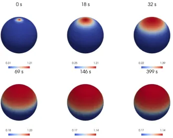
Sphere

Our first three-dimensional geometry on which we solve the BSWP model (5)-(8) is the sphere which is the simplest possible three-dimensional shape. We consider a radius of 5µm, which is the radius used in the simulations of the WP model [37]. We consider εb= 0.154 in (44) andσ2= 0.5µm2 in (45). The perturbation of the homogeneous state is strong enough to trigger polarisation: from this small region, a propagative activation is started in all directions. This will be finally pinned in about 100 seconds, resulting in a stable active area. In Figure 7 we show the evolution ofaand in Figure 8 the temporal evolution of the masses ofaandb which become constants when the propagation gets pinned.

Figure 7: Numerical simulations of the BSWP model (5)-(8) on a sphere: The active form of Rho GTPase a propagating from a ”stimulating” initial condition (17) over a sphere. The numerical solution reaches a stable configuration after about 100 seconds. See text for further details.

6.2

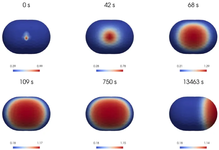
Capsule

Figure 8: Variation in time of the total mass of active (left) and inactive (right) GTPases of the numerical solution shown in Figure 7. The initial decrease in the mass of ais due to the attraction of the solution towards the smaller value a1(b) in most of its domain. Consequently we observe an initial increase of the mass of b. The mass of astarts increasing with the spreading of its activity over the surface, which reduces the mass ofb. After about 100 seconds the two components approach the equilibrium in mass.

Figure 9: Numerical simulations of the BSWP model (5)-(8) on a capsule. The solution a is here reported at several time steps: a small area in the lateral side of the capsule is activated, causing the activation of the entire lateral section which reaches its maximal size after around 120 seconds. Eventually, after a very long time, the activated area moves towards one of the spherical caps of the domain.

6.3

Polarised cell shape

of the domain and gets pinned in about 10 minutes.

Figure 10: The surface of a polarised cell shaped domain. The domain has been discretised with 5362 tetrahedrons which induced a surface discretisation with 3044 triangles.

Figure 11: Numerical simulation of the BSWP model (5)-(8) on a more complex domain, caricature of a polarised cell. The numerical results show the solution aat different stages of the polarisation process: a small area in two of the five tips of the domain is activated and this generates two propagating fronts which merge together in about 4 minutes. The activated area stabilises covering the whole front of the domain in about 10 minutes. A video illustrating the wave pinning process is provided in the supplementary material.

starts disappearing. This leads to a winning tip, which continues enlarging on its side, until final stabilisation.

Figure 12: Numerical simulation of the BSWP model (5)-(8) on a domain mimicking a polarised cell. In this simulation the external tips are activated. Two active waves are generated and start propagating on the surface. After about 5 minutes the competition effects between the two active patches start being visible, and one active region (left tip) starts reducing its size, until it disappears completely. Disappearing and stabilisation of the remaining active area occur after more than 30 minutes. Competition in two-dimensional wave pinning model was very recently investigated in [6].

In all previous simulations, we have used suitable initial conditions in the form of perturbations of the spatially homogeneous profile ofa. This has been shown to be enough to give rise to polarisation, in the numerical results, as well as for the asymptotic and local perturbation analysis. However, similar perturbations can be induced by perturbing the reaction (7). Indeed, in most of the papers simulating the WP model, polarisation was initiated from a stimulus included in the reaction function, rather than a stimulus in the initial conditions, which were, in turn, spatially homogeneous. Following this latter approach, the BSWP model is given by equations (5)-(8) with reaction

f(a, b) =ωk0+

γa2 K2_+a2

b−βa+ωksb, x∈Γ. (47)

where ks_=ks_{(x, t) is an arbitrary function, generally non-negative until a certain timet}

a homogeneous stimulus of 0.03 s−1 _{for 20 seconds. This induces a rapid local activation of the} ellipsoidal volume on the top of the cell, with noticiable effects within the first 5 seconds. The high

aconcentration starts increasing and sharpening the fronts, and successively it spreads towards the rear of the domain. Our simulation confirms the interesting geometry-induced self-polarisation ability also for the three-dimensional case.

Figure 13: Numerical simulation of the BSWP model (5)-(6) and (8) with reaction kinetics (47) on a domain mimicking a polarised cell. We apply a constant stimulus ks_{(x, t) = 0.03 s}−1 _{until time}

tS=20 s which induces an activation at the level of the nucleus-shaped volume. From here, a wave starts, covering the whole rear. In about 20 minutes the BSWP model has reached its steady state, with the rear having high levels of active GTPase.

7

Discussion

In this paper, we have presented a three-dimensional extension of the wave pinning model in a bulk-surface setting, in which membrane-bound GTPase and cytosolic GTPase are spatially localised and their interactions occur on the cell surface. The model describes cell polarisation through a minimal circuit of GTPase switching between active and inactive forms as well as between the membrane and the cytosol. In our work we were able to show many analogies to the classical wave pinning model [37, 38, 57] not previously shown in three-dimensional domains.

parameters mapping have been investigated in Section 4, where we have highlighted how polarisation behavior is more probable in complex domains. This has been done using local perturbation analysis which allows a reduction to a ODE system. Finally, using the bulk-surface finite element method, presented in Section 5, we computed numerical solutions of the BSWP model on different domains. An interesting result has been obtained from the model over a capsule-shape domain, where long time behavior of the model has been simulated, showing another common property of the classical wave pinning model derived by Mori et al. [37], noted in [57]: the high active concentration region moves very slowly from its apparent stable steady state towards more rounded areas, until it covers one of the spherical caps of the capsule.

Simulations have been done also on a more complex geometry mimicking a polarised cell-like shape. We showed competition between different highly active areas, as previously reported for the classical wave pinning mechanism [6]. In addition, we show how geometry plays a crucial role on the spontaneous polarisation in our three-dimensional BSWP model, as reported in the two-dimensional case by Gieseet al. [19]. In the latter case, the asymmetric geometry of the domain plays a crucial role in enhancing activation of the GTPases. Indeed, activation was induced by a spatial homogeneous stimulus, but its effects appear well localised in specific areas of the surface.

Positive feedback, known to be a biological feature of Rho GTPases [22], has been confirmed as a key player also in the new formulation of the model. It is represented by the Hill function in (7), but many other nonlinear choices are possible. Identification of Rho GTPase feedback is an extremely interesting task and hopefully coordinated efforts between biologists and mathematicians can lead the way to a more complete understanding of cell polarisation and migration.

We expect the BSWP (5)-(8) to be a starting point for a more complete work, in which the biochemical mechanisms shown above are coupled with mechanical properties of the cell, such as membrane tension and migration. Indeed, in real cells, GTPase concentration would lead to shape changes, through cytoskeleton interactions. The classical wave pinning model has been already coupled to mechanistic models for membrane tension [58] and cell migration [4, 57]. In these latter works the migrating cell, instead of keeping a straight direction, was turning over one side. This corresponded to the slow motion of the polarised area, as discussed in the Section 6.2 and in Figure 9. In view of this and taking into account the influence of the geometry of the domain, it can be of interest to extend these results and investigate how the bulk-surface approach influences the mechanical properties. Indeed, as reported in Figure 9, the slow motion appears to be much slower with respect to the one reported in the literature [57] and, in a reasonable amount of time, the turning effect might not be noticeable. As well, the effects of the geometry reported in Section 4 might play an important role on evolving domains describing more accurately migrating cells, in which the parameterω=|Ω|/|Γ|is subject to changes in time.

Another interesting extension of this study is whether it is possible to achieve similar mechanisms in a bulk-surface model with three species, when membrane recruitment of cytosolic GTPase is taken into account. This idea of GTPase model has been presented in [49], but the polarisation mechanisms were Turing-type.

Data accessibility

The authors declare no use of primary data as a result there is no supporting material to present in association to the results pertained by the current manuscript.

Acknowledgments

EP/K032208/1. LEK is supported by an NSERC Discovery Grant. SP is supported in part by an NSERC Discovery Grant. AM was partially supported by a fellowship from the Simons Foundation. AM is a Royal Society Wolfson Research Merit Award Holder, generously supported by the Wolfson Foundation.

References

[1] _{Alnæs, M., Blechta, J., Hake, J., Johansson, A., Kehlet, B., Logg, A., Richardson,} C., Ring, J., Rognes, M. E., and Wells, G. N. The FEniCS project version 1.5. Archive of Numerical Software 3, 100 (2015), 9–23.

[2] _{Altschuler, S. J., Angenent, S. B., Wang, Y., and Wu, L. F.} On the spontaneous emergence of cell polarity. Nature 454, 7206 (2008), 886.

[3] Andrew, N., and Insall, R. H. Chemotaxis in shallow gradients is mediated independently of PtdIns 3-kinase by biased choices between random protrusions.Nature cell biology 9, 2 (2007), 193.

[4] _{Camley, B. A., Zhao, Y., Li, B., Levine, H., and Rappel, W.-J.}Crawling and turning in a minimal reaction-diffusion cell motility model: coupling cell shape and biochemistry. Physical Review E 95, 1 (2017), 012401.

[5] _{Chang, Y.-C., Nalbant, P., Birkenfeld, J., Chang, Z.-F., and Bokoch, G. M.} GEF-H1 couples nocodazole-induced microtubule disassembly to cell contractility via RhoA.Molecular Biology of the Cell 19, 5 (2008), 2147–2153.

[6] _{Chiou, J.-G., Ramirez, S. A., Elston, T. C., Witelski, T. P., Schaeffer, D. G.,} and Lew, D. J. Principles that govern competition or co-existence in Rho-GTPase driven polarization. PLoS Computational Biology 14, 4 (2018), e1006095.

[7] DerMardirossian, C., and Bokoch, G. M. GDIs: central regulatory molecules in Rho GTPase activation. Trends in Cell Biology 15, 7 (2005), 356–363.

[8] _{Diegmiller, R., Montanelli, H., Muratov, C. B., and Shvartsman, S. Y.} Spherical Caps in Cell Polarization. Biophysical Journal 115 (2018), 26–30.

[9] _{Drubin, D. G., and Nelson, W. J.} Origins of cell polarity. Cell 84, 3 (1996), 335–344.

[10] _{Dziuk, G., and Elliott, C. M.} Finite element methods for surface PDEs. Acta Numerica 22 (2013), 289–396.

[11] _{Edelstein-Keshet, L., Holmes, W. R., Zajac, M., and Dutot, M.} From simple to detailed models for cell polarization. Philosophical Transactions of the Royal Society of London B: Biological Sciences 368, 1629 (2013), 20130003.

[12] Elliott, C. M., and Ranner, T. Finite element analysis for a coupled bulk–surface partial differential equation. IMA Journal of Numerical Analysis 33, 2 (2013), 377–402.

[13] Etienne-Manneville, S.Polarity proteins in migration and invasion.Oncogene 27, 55 (2008), 6970.

[14] _{Evans, L. C.} Partial differential equations. American Mathematical Society, 2010.

[15] _{Fife, P. C., and McLeod, J. B.}The approach of solutions of nonlinear diffusion equations to travelling front solutions. Archive for Rational Mechanics and Analysis 65, 4 (1977), 335–361.

[17] _{Fujiwara, S., Ohashi, K., Mashiko, T., Kondo, H., and Mizuno, K.} Interplay between Solo and keratin filaments is crucial for mechanical force–induced stress fiber reinforcement.

Molecular Biology of the Cell 27, 6 (2016), 954–966.

[18] _{Geuzaine, C., and Remacle, J.-F.} Gmsh: A 3-D finite element mesh generator with built-in pre-and post-processing facilities. International Journal for Numerical Methods in Engineering 79, 11 (2009), 1309–1331.

[19] Giese, W., Eigel, M., Westerheide, S., Engwer, C., and Klipp, E. Influence of cell shape, inhomogeneities and diffusion barriers in cell polarization models. Physical Biology 12, 6 (2015), 066014.

[20] _{Goryachev, A. B., and Leda, M.}Many roads to symmetry breaking: molecular mechanisms and theoretical models of yeast cell polarity. Molecular Biology of the Cell 28, 3 (2017), 370–380.

[21] _{Goryachev, A. B., and Pokhilko, A. V.} Dynamics of Cdc42 network embodies a Turing-type mechanism of yeast cell polarity. FEBS Letters 582, 10 (2008), 1437–1443.

[22] _{Graessl, M., Koch, J., Calderon, A., Kamps, D., Banerjee, S., Mazel, T., Schulze,} N., Jungkurth, J. K., Patwardhan, R., Solouk, D., Hampe, N., Hoffmann, B., Leif, D., and Nalbant, P. An excitable Rho GTPase signaling network generates dynamic subcel-lular contraction patterns. Journal of Cell Biology (2017).

[23] Guilluy, C., Garcia-Mata, R., and Burridge, K. Rho protein crosstalk: another social network? Trends in Cell Biology 21, 12 (2011), 718–726.

[24] Hodge, R. G., and Ridley, A. J. Regulating Rho GTPases and their regulators. Nature Reviews Molecular Cell Biology 17, 8 (2016), 496.

[25] _{Holmes, W. R.} An efficient, nonlinear stability analysis for detecting pattern formation in reaction diffusion systems. Bulletin of Mathematical Biology 76, 1 (2014), 157–183.

[26] _{Holmes, W. R., and Edelstein-Keshet, L.} Analysis of a minimal Rho-GTPase circuit regulating cell shape. Physical Biology 13, 4 (2016), 046001.

[27] _{Holmes, W. R., Mata, M. A., and Edelstein-Keshet, L.} Local perturbation analysis: A computational tool for biophysical reaction-diffusion models. Biophysical Journal 108, 2 (2015), 230–236.

[28] Jilkine, A., and Edelstein-Keshet, L. A comparison of mathematical models for polar-ization of single eukaryotic cells in response to guided cues. PLoS Computational Biology 7, 4 (2011), e1001121.

[29] Kozlov, M. M., and Mogilner, A. Model of polarization and bistability of cell fragments.

Biophysical Journal 93, 11 (2007), 3811–3819.

[30] _{Ladoux, B., M`ege, R.-M., and Trepat, X.} Front–rear polarization by mechanical cues: From single cells to tissues. Trends in Cell Biology 26, 6 (2016), 420–433.

[31] _{MacDonald, G., Mackenzie, J. A., Nolan, M., and Insall, R.}A computational method for the coupled solution of reaction–diffusion equations on evolving domains and manifolds: Application to a model of cell migration and chemotaxis. Journal of Computational Physics 309

(2016), 207–226.

[32] _{Madzvamuse, A., and Chung, A.}Analysis and simulations of coupled bulk-surface reaction-diffusion systems on exponentially evolving volumes. Mathematical Modelling of Natural Phe-nomena 11, 5 (2016), 4–32.

[34] _{Madzvamuse, A., Chung, A. H., and Venkataraman, C.}Stability analysis and simulations of coupled bulk-surface reaction–diffusion systems. Proceedings of the Royal Society of London A 471, 2175 (2015), 20140546.

[35] _{Mar´ee, A. F., Jilkine, A., Dawes, A., Grieneisen, V. A., and Edelstein-Keshet,} L. Polarization and movement of keratocytes: a multiscale modelling approach. Bulletin of Mathematical Biology 68, 5 (2006), 1169–1211.

[36] Mayor, R., and Carmona-Fontaine, C. Keeping in touch with contact inhibition of loco-motion. Trends in Cell Biology 20, 6 (2010), 319–328.

[37] _{Mori, Y., Jilkine, A., and Edelstein-Keshet, L.} Wave-pinning and cell polarity from a bistable reaction-diffusion system. Biophysical Journal 94, 9 (2008), 3684–3697.

[38] _{Mori, Y., Jilkine, A., and Edelstein-Keshet, L.} Asymptotic and bifurcation analysis of wave-pinning in a reaction-diffusion model for cell polarization. SIAM Journal on Applied Mathematics 71, 4 (2011), 1401–1427.

[39] _{Nelson, D. L., Lehninger, A. L., and Cox, M. M.} Lehninger principles of biochemistry. Macmillan, 2008.

[40] _{Nelson, W. J.} Adaptation of core mechanisms to generate cell polarity. Nature 422, 6933 (2003), 766.

[41] Novak, I. L., Gao, F., Choi, Y.-S., Resasco, D., Schaff, J. C., and Slepchenko, B. M. Diffusion on a curved surface coupled to diffusion in the volume: Application to cell biology. Journal of Computational Physics 226, 2 (2007), 1271–1290.

[42] _{Ohashi, K., Fujiwara, S., and Mizuno, K.} Roles of the cytoskeleton, cell adhesion and rho signalling in mechanosensing and mechanotransduction. The Journal of Biochemistry 161, 3 (2017), 245–254.

[43] _{Otsuji, M., Ishihara, S., Kaibuchi, K., Mochizuki, A., Kuroda, S., et al.} A mass conserved reaction–diffusion system captures properties of cell polarity. PLoS computational biology 3, 6 (2007), e108.

[44] _{Postma, M., Bosgraaf, L., Loovers, H. M., and Van Haastert, P. J.} Chemotaxis: signalling modules join hands at front and tail. EMBO Reports 5, 1 (2004), 35–40.

[45] Quarteroni, A., Sacco, R., and Saleri, F. Numerical mathematics, vol. 37. Springer Science & Business Media, 2010.

[46] Ramirez, S. A., Raghavachari, S., and Lew, D. J. Dendritic spine geometry can localize GTPase signaling in neurons. Molecular Biology of the Cell 26, 22 (2015), 4171–4181.

[47] _{Rappel, W.-J., and Edelstein-Keshet, L.}Mechanisms of cell polarization.Current Opinion in Systems Biology 3 (2017), 43–53.

[48] _{R¨atz, A., and R¨oger, M.}Turing instabilities in a mathematical model for signaling networks.

Journal of Mathematical Biology 65, 6-7 (2012), 1215–1244.

[49] _{R¨atz, A., and R¨oger, M.} Symmetry breaking in a bulk–surface reaction–diffusion model for signalling networks. Nonlinearity 27, 8 (2014), 1805.

[50] _{Reig, G., Pulgar, E., and Concha, M. L.} Cell migration: from tissue culture to embryos.

Development 141, 10 (2014), 1999–2013.