1
FREE-SURFACE EFFECTS ON MULTIPLE SHIPS
1TRAVELLING WITH DIFFERENT SPEEDS
2Zhi-Ming Yuan*, †, Liang Li† and Ronald W. Yeung‡,* 3
*Jiangsu University of Science and Technology, China. 4
†University of Strathclyde, UK 5
‡University of California at Berkeley, USA 6
*Corresponding author, E-mail: [email protected], Tel.: +1 (510) 642-7
8347 8
9 10
ABSTRACT 11
Ships often have to pass each other in proximity in harbor area and waterways 12
in dense shipping traffic environment. Hydrodynamic interaction occurs when 13
a ship is overtaking (or being overtaken) or encountering other ships. Such an 14
interactive effect could be magnified in confined waterways, e.g. shallow and 15
narrow rivers. Since Yeung (1978) published his initial work on ship-interaction 16
in shallow water, progress on unsteady interaction among multiple ships has 17
been slow though steady over the following decades. With some exceptions, 18
nearly all the published studies on ship-to-ship problem neglected free-surface 19
effects, and a rigid wall condition has often been applied on the water surface 20
as the boundary condition. When the speed of the ships is low, this assumption 21
is reasonably accurate, as the hydrodynamic interaction is mainly induced by 22
near-field disturbances. However, in many maneuvering operations, the en-23
countering or overtaking speeds are actually moderately high (Froude number 24
Fn>0.2, where 𝐹𝑛 ≡ 𝑈/√𝑔𝐿, U is ship speed, g the gravitational acceleration and
25
L the ship length), especially when the lateral separation between ships is the 26
order of ship length. Here, the far-field effects arising from ship waves can be 27
important. The hydrodynamic interaction model must take into account of the 28
surface-wave effects. 29
Classical potential-flow formulation is only able to deal with the boundary 30
value problem (BVP) when there is only one speed involved in the free-surface 31
boundary condition. For multiple ships travelling with different speeds, it is not 32
possible to express the free-surface boundary condition by a single velocity po-33
tential. Instead, a superposition method can be applied to account for the veloc-34
ity field induced by each vessel with its own and unique speed. The main objec-35
tive of the present paper is to propose a rational superposition method to handle 36
the unsteady free-surface boundary condition containing two or more speed 37
terms, and validate its feasibility in predicting the hydrodynamic behaviour of 38
the ships during overtaking or encountering operations. The solution methodol-39
ogy used in the present paper is a three-dimensional boundary-element method 40
(BEM) based on a Rankine-type (infinite-space) source function, initiated intro-41
duced in Bai & Yeung (1974). The numerical simulations are conducted by using 42
an in-house developed multi-body hydrodynamic interaction program "MHy-43
dro". Waves generated and forces (or moments) are calculated when ships are 44
encountering or passing each other. Published model-test results are used to 45
validate our calculations and very good agreement has been observed. The nu-46
merical results show that free-surface effects need to be taken into account for 47
2
Keywords: Free-surface effect; ship-to-ship problem; hydrodynamic interaction;
49
encountering and overtaking operation; ship manoeuvring. 50
51 52
1 INTRODUCTION
53
The interaction between two or more ships involved in encountering or overtak-54
ing manoeuvring is a classical hydrodynamic problem. Due to the interaction 55
forces, a ship may deviate from its original course and collide with the other 56
ships. The interaction effects are aggravated when the ships are manoeuvring 57
in confined waterways, or when the ships are travelling with high speed. 58
Ship-to-ship problem has been widely studied over the last few decades. No mat-59
ter which kind of methods are used, at least one or more of the following im-60
portant assumptions are often adopted to simplify the problem: 61
1) The fluid is ideal and the viscous effects are neglected. 62
2) The speed is low and the free-surface effects are negligible (rigid-wall 63
free-surface is applicable). 64
3) The ships are slender. 65
4) The shedding of cross-flow vorticity is either ignored, or idealized in a 66
manner similar to thin-wing theory. 67
During1960s-1990s, the slender-body theory has been widely popular to predict 68
the hydrodynamic interaction between multiple ships (Collatz, 1963; Dand, 69
1975; Kijima and Yasukawa, 1985; Tuck, 1966; Tuck and Newman, 1974; 70
Varyani et al., 1998; Yeung, 1978). All of the assumptions mentioned above are 71
adopted in these studies. These assumptions significantly simplified the math-72
ematical model and led to a high-efficiency numerical calculation. For conven-73
tional ships travelling at relatively low Froude numbers, the numerical calcula-74
tions based on strip theory showed a fairly good prediction of the sway force and 75
yaw moment on ships during overtaking or meeting operations. To account for 76
the three-dimensional effects and remove the geometrical idealization described 77
above (Assumption 3)), Korsmeyer et al. (1993) adopted a three-dimensional 78
panel method, which is applicable to any number of arbitrary shaped bodies in 79
arbitrary motions. Pinkster (Pinkster, 2004) extended Korsmeyer’s method with 80
implementation of a model to account for the free-surface effects partially. His 81
model was restricted to simulating the effect of a passing ship on a moored ship. 82
Only the low frequency seiche or solitary waves were taken into account, while 83
the more important far-field waves or so-called Kelvin waves were neglected. Therefore, 84
his conclusions on free-surface effects could not cover the general ship-to-ship 85
operations. More recently, the three-dimensional panel method has been more 86
commonly used (Söding and Conrad, 2005; Xiang and Faltinsen, 2010; Xu et al., 87
2016; Zhou et al., 2012). However, no effort has yet been made to investigate the 88
effects of unsteady free-surface waves on interaction forces. The general conclu-89
sion drawn from these studies is that the potential flow solver could provide a 90
good prediction of interaction forces on ships travelling at relatively low Froude 91
numbers. Benefitted from improving CFD (Computational Fluid Dynamics) 92
technology, the viscous effects on ship-to-ship problem have been investigated 93
by various turbulence models (Jin et al., 2016; Sian et al., 2016; Zou and 94
Larsson, 2013b). In these studies, the free-surface effects are either neglected 95
(Zou and Larsson, 2013b) or treated simply as a steady problem (Jin et al., 2016; 96
3
free-surface waves produced by two or more ships moving with different speeds. 98
Mousaviraad et al. (2016b) analyzed the ship-ship interaction experiments both 99
in calm water and waves. They also run the URANS simulations, in which the 100
free-surface boundary condition was considered (Mousaviraad et al., 2016a). 101
However, these studies focus more on the hydrodynamic forces. The result of 102
free-surface elevation was neither measured in the model tests nor presented in 103
the CFD simulations. The demand in computational power when more than one 104
ship is passing can be the bottleneck if real-time applications should be needed. 105
All the above mentioned studies adopted the assumption that the encountering 106
or overtaking speed is low. Therefore, the unsteady free-surface wave effect is 107
not essential. This assumption significantly reduces the complexity of unsteady 108
ship-to-ship problem. But in the real manoeuvring practice, the encounter speed 109
is not always low. The importance of the free-surface effect is determined by 110
whether the far-field waves generated by a ship could propagate to the other 111
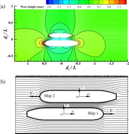
ships. At low Froude number, the amplitude of the far-field waves is very small. 112
These far-field waves are dissipated before they propagate to the far-field, as 113
shown in Fig. 1(a). Fig. 1 (b) shows the sketch of flow passing the gap between 114
two ships. The flow is compressed to pass through the narrow gaps between two 115
ships with relative higher velocity. According to Bernoulli's principle, the accel-116
erated fluid velocity could result in a decrease in pressure distribution in the 117
gap, therefore inducing hydrodynamic interaction forces (or moments). In this 118
low-speed case, the free-surface elevation and the hydrodynamic interaction are 119
mainly determined by the near-field disturbance. As the speed increases, the 120
far-field waves can be observed apparently. The far-field wave patterns gener-121
ated by two pressure disturbances moving towards opposite direction are shown 122
in Fig. 2 (a). The encounter process of these two disturbances is time-dependent. 123
It can be anticipated when a disturbance is in the other’s wake region, the hy-124
drodynamic interaction will be unavoidable. In the port or inland waterways, 125
the hydrodynamic interaction between three-dimensional vessels is also con-126
ceivable by the propagation of the far-field waves. The wave elevation reflects 127
the pressure distribution on water surface. The interaction occurs when the 128
waves produced by a ship strike the others, therefore modifying the pressure 129
distribution over their immersed body surfaces. Thus, the hydrodynamic inter-130
action can be apparently observed by wave interference on free water surface. 131
Benefit from satellite and imaging technology, we can observe the wave inter-132
ference phenomenon by analyzing high resolution satellite images. The encoun-133
tering and overtaking process of two real ships are shown in Fig. 2 (b) and (c) 134
respectively. These images show the far-field wave interference, which indicates 135
the ship-to-ship operation is not only limited at low Froude number. Even 136
though the transverse separation between the ships is large, the wave interfer-137
ence effect can still result in strong hydrodynamic interaction. The rigid free-138
surface is not capable to predict the hydrodynamic interactions induced by far-139
field waves. A new methodology should be proposed to deal with the free-surface 140
boundary condition.
141
The main challenge of imposing a non-rigid free-surface condition arises 142
from the speed term in the body boundary condition (See.Eq. (16) later). For 143
multiple ships travelling with various speeds, it is not possible to express the 144
free-surface boundary condition by a single velocity potential (unless one uses 145
an earth-fixed coordinate system as in Yeung (1975)). A superposition method, 146
however, can be applied to account for the velocity potentials induced by each 147
4
appearing in free-surface boundary condition, Yuan et al. (2015) proposed an 149
uncoupled method based on the superposition principle. Therein, the speed dif-150
ference of two ships was assumed to be small. Thus, the free-surface condition 151
could be treated (arguably) as steady-state problem. This method is not appli-152
cable to predict the interaction forces when ships’ speeds are not the same, or 153
when two ships are moving towards each other. In these cases, the unsteady 154
effect becomes essential and the time-dependent terms must be taken into ac-155
count. In the present study, we will extend Yuan’s method to the time domain 156
and discuss the importance of free-surface effects on multi-ship problem. 157
Fig. 1. (a), wave patterns produced by two ships travelling at low Froude number (Fn
158
= 0.043) (Yuan et al., 2015). (b), sketch of flow passing the gap between two ships.
159
dl/ L
dt
/
L
1 0.5 -0 -0.5 -1 -1.5 -2
-0.5 0 0.5
1 Wave height (mm): -2.0 -1.5 -1.1 -0.6 -0.1 0.3 0.8 1.3
Ship 2
y2
Ship 1
x2
o2
y1
x1
o1
U1
U2
(a) (a)
[image:4.595.170.424.205.469.2]5
Fig. 2. (a), sketch showing the transverse and divergent waves generating by two
160
pressure disturbances moving towards opposite direction. (b) and (c), satellite image of
161
ship wakes taken from the Google Earth database. (b), two ships encountering at
162
Dordtse Kil, The Netherlands
163
(https://www.google.com/maps/@51.7519406,4.6291446,652a,35y,75.15h,8.71t/data=!3
164
m1!1e3?hl=en). (c), two ships overtaking at Lek, Netherlands
165
(https://www.google.com/maps/@51.9953387,5.0694056,298a,35y,325.35h/data=!3m1!1
166
e3?hl=en). The Froude number of the vessels in the lower part of (b) and upper part of
167
(c) is Fn ≈ 0.15.
168
2 THE BOUNDARY VALUE PROBLEM
169
[image:5.595.169.423.69.342.2]170
Fig. 3. Coordinate systems. 171
Consider N ships moving at speeds Uj (j = 1, 2, …, N) with respect to a space-172
fixed reference frame 𝐱 = (𝑥, 𝑦, 𝑧) in an inviscid fluid of depth h as shown in Fig. 173
3. A right-handed Cartesian coordinate system 𝐱𝐣= (𝑥𝑗, 𝑦𝑗, 𝑧𝑗) (j = 1, 2, …, N) is 174
fixed to each ship with its positive xj-axis pointing towards the bow, positive z-175
axis pointing upwards and zj = 0 being the undisturbed free-surface. Let Φ (x, 176
t) be the velocity potential describing the disturbances generated by the forward 177
40 m
40 m
x2 O2
y2
z2
T
2
y1
z1
x1
O1
U1
yn zn
xn On
U2
Un y
z
O x
dl
dt
B1
BN
B2
(b)
[image:5.595.205.411.487.653.2]6
motion of the ships and ζ (x, y, t) be the free-surface wave elevation. In the fluid 178
domain, the total velocity potential Φ satisfies the Laplace equation 179
2
( , )t 0
x (1)
180
The fluid pressure, 𝑝(𝐱, 𝑡), is given by Bernoulli’s equation 181
0
1 ( , )
2
p t gz p
t
x (2)
182
where ρ is the fluid density, p0 is the atmospheric pressure, which is used as a 183
reference pressure and assumed to be constant. Assuming there is no overturn-184
ing and breaking waves on the free-surface, we can use this Eulerian description 185
of the flow to describe the free-surface motion. The free-surface elevation is 186
given by z = ζ (x, y, t). A fluid particle on the free-surface is assumed to stay on 187
the free-surface, which leads to the following kinematic free-surface boundary 188
condition: 189
0D z
Dt , on z = ζ (3)
190
The material derivative in Eq. (3) is given by: 191
D
Dt t
(4)
192
The dynamic free-surface condition is that the fluid pressure equals the con-193
stant atmospheric pressure p0 on the surface, since the position of the free-194
surface is unknown. According to Bernoulli’s equation Eq. (2), the dynamic free-195
surface boundary condition can be written as 196
1
0
2 gz
t
, on z = ζ (5)
197
By applying Taylor series expanded about z = 0 and only keeping the linear 198
terms, the dynamic and kinetic free-surface conditions can be linearized as 199
0
t z
, on z = 0 (6)
200
0
g
t
, on z = 0 (7)
201
Combining Eq. (6) and (7), we obtain the free-surface boundary condition: 202
2
2 g 0
t z
, on z = 0 (8)
203
It should be noted the free-surface ζ can be found from Eq. (7) when the velocity 204
potential Φ is known. On the wetted body surface, the no-flux boundary condi-205
tions are used, and the following ‘exact’ boundary condition can be formulated: 206
j x j
U n
n
, on Bj, where j = 1, 2, …, N (9)
207
where ∂/∂n is the derivative along the normal vector 𝐧 = (𝑛𝑥, 𝑛𝑦, 𝑛𝑧) into the 208
7
Assuming the disturbance of the fluid is small, we represent the total velocity 210
potential produced by the presence of all ships in the fluid domain in a space-211
fixed frame to satisfy the following superposition principle: 212
1
( , ) ( , )
N
j j
t t
x
x , j = 1, 2, …, N (10)213
where Φj (x, t) is the velocity potential produced by the presence of ship j moving 214
with Uj, while the remaining ships are momentarily stationary in this frame. 215
For the linear problem, the body-fixed coordinate system 𝐱𝐣= (𝑥𝑗, 𝑦𝑗, 𝑧𝑗) (j = 1, 2,
216
…, N) is used to solve the BVP for N vessels in concurrent motion. The relation 217
between the body- and space-fixed coordinate system is straightforward, viz. 218
j j
x x U t, j = 1, 2, …, N (11) 219
Let ϕj (xj, t) represents Φj (x, t) in the body-fixed coordinate system, the following 220
relation can be obtained 221
j
j j
j
d
U
dt t x
(12)
222
The velocity potential ϕj satisfies the Laplace equation and body ‘exact’ bound-223
ary condition: 224
2
( , ) 0
j t
xj , j = 1, 2, …, N (13)
225
j
ijUj nx j
n
, on Bi, where i, j = 1, 2, …, N (14) 226
The Kronecker delta δij is the quantity defined by 227
1
0
ij
i j i j
(15)
228
Substituting Eq. (12) into the linearized free-surface condition in Eq. (8), we ob-229
tain the linearized free-surface condition in the body-fixed coordinate system 230
2 2 2
2
2 2 2 0
j j j j
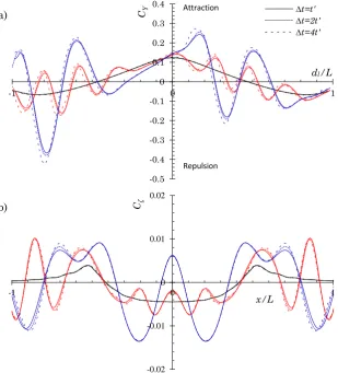
j j
j j j
U U g
t x t x z
, on z = 0 (16)
231
The boundary condition on the sea bottom and side walls, if any, can be ex-232
pressed as 233
0 j
n
(17)
234
Besides, a radiation condition is imposed on the control surface to ensure that 235
waves vanish at upstream infinity 236
2 2
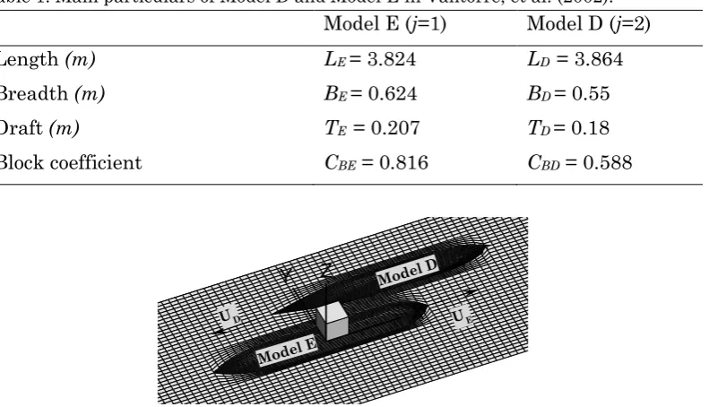
0, 0
j j as xj yj
(18)
237
where ζj is the wave elevation as seen in the j-th body-fixed frame and is given 238
8
3 NUMERICAL SOLUTIONS
240
Eqs. (13) - (18) define a complete set of BVP. Each one of BVP is time-dependent 241
but can be solved individually and independently; only a single speed of ship j 242
appears in the free-surface condition in Eq.(16). The coupled problem is decou-243
pled into N independent BVPs. At each time instant, the BVP in Eqs. (13) - (18) 244
can be solved numerically. Following the work of Hess & Smith (1964), the 245
boundaries are discretized into a number of quadrilateral panels with constant 246
source density σ(ξj), where 𝝃𝒋= (𝜉𝑗, 𝜂𝑗, 𝜍𝑗) is a position vector on the boundaries
247
in the j-th body-fixed frame and the free-surface (Bai & Yeung, 1974). Let 𝐱𝐣=
248
(𝑥𝑗, 𝑦𝑗, 𝑧𝑗) denote a point inside the fluid domain or on the boundary surface, the 249
velocity potential ϕ can be expressed by a source distribution on the boundary 250
of the fluid domain 251
, j = 1, 2, …, N (19) 252
where G=1/r is the Rankine-type source function, with r being the distance be-253
tween ξj and xj. More detailed numerical implementation on the solution of BVP
254
can be found in Yuan et al. (2014b). The same in-house developed program MHy-255
dro is deployed in the present study as the framework to investigate ship hydro-256
dynamics in restricted waterways. Special care should be taken to implement a 257
suitable open boundary condition to satisfy Eq. (18). In numerical calculations, 258
the computational domain is always truncated at a distance away from the ship 259
hull. In general, waves will be reflected from the truncated boundaries and con-260
taminate the flow in the computational domain. In the present study, a second-261
order upwind difference scheme is applied on the free-surface to obtain the time 262
and spatial derivatives: 263
264
2
2 2 4 3 2 1
1 1 11 9
2 6
4 2 4
j
j j j j j
k k k k k k
x x
xj xj xj xj xj xj
265
(20) 266
Here k refers to the panel number. According to Bunnik (1999) and Kim et al. 267
(2005), Eq. (18) can be satisfied consequently by applying Eq.(20). It should be 268
noted that the 2nd order upwind difference scheme is applied at each body-fixed 269
frame locally. This is essential to deal with ships travelling towards opposite 270
directions. 271
For each individual velocity potential ϕj, the BVP is unsteady due to the time-272
dependent terms in Eq. (16). In previous studies on ship-to-ship interaction 273
problem (Xu et al., 2016; Yeung, 1978; Yeung and Tan, 1980), within the frame-274
work of potential-flow theory, the BVP was not in time domain as the free-sur-275
face condition was assumed to be rigid. It was solved independently at each in-276
dividual time step. The unsteady effect was only considered in the pressure cal-277
culations in Eq. (27). The unsteady interaction forces calculated in these studies 278
are not exactly ‘unsteady’, since the velocity potential at each time step is not 279
time dependent. The velocity potential obtained at tn is not related to that ob-280
tained at tn-1, and it will also not determine that at tn+1. In the present study, 281
the unsteady BVP will be solved in time domain by an iteration scheme. The 282
essential steps are: 283
1
( ) ( ) ( , )
N f c b j
j
S S S
G ds
j j j j
9
1. Determine the initial condition. We assume that at the initial stage of 284
ship-to-ship operation, the moving ships are sufficiently far apart so that 285
their interactions are negligible. Thus, the time dependent terms are re-286
moved from the free-surface condition in Eq. (16), and we have 287
*
* 2 2 2 0 k k j j j j j U g x z (21)
288
Here (𝜙𝑗𝑘)∗ is the time-independent velocity potential at the time step k.
289
The computational domain and the corresponding panel distribution at 290
each time step k can be constructed and the steady BVP in Eqs. (13) to 291
(15), (21), (17) and (18) can be solved straightforwardly by using the Ran-292
kine source panel method. The time-independent velocity potential (𝜙𝑗𝑘)∗
293
can be obtained, which will be used as the initial guess to calculate the 294
time derivatives of unsteady velocity potential 𝜙𝑗𝑘 in Eq. (22).
295 296
2. By applying the second-order backward difference scheme, the time de-297
rivatives in Eq. (16) can be calculated according to the following formulas 298
* 1 * 2 *
2
* 1 * 2 * * 3 *
2 2
1 3 1
2
2 2
1
2 5 4
k
j k k k
j j j
k
j k k k k
j j j j j
t t t t
(22) 2993. Substituting Eq. (22) into Eq. (16), the following time-domain free-sur-300
face condition can be obtained 301
2 2
2
2 2 2 0
k k k k k
j j j j j
j j
j j j
U U g
t t x x z
(23)
302
Solving the unsteady BVP in Eqs. (13) to (15), (23), (17) and (18), we can 303
obtain the unsteady velocity potential 𝜙𝑗𝑘. Residual errors of time
deriv-304
atives of |(𝜙𝑗𝑘)∗− 𝜙
𝑗𝑘| can be evaluated. If |(𝜙𝑗𝑘)∗− 𝜙𝑗𝑘| < 𝜀, the iteration
305
stops and 𝜙𝑗𝑘 will be used to calculated the pressure and wave elevation.
306
Otherwise, (𝜙𝑗𝑘)∗ in Eq. (22) will be replaced by the newly obtained 𝜙 𝑗𝑘,
307
and the iteration continues until |(𝜙𝑗𝑘)∗− 𝜙
𝑗𝑘| < 𝜀. It is known that the
308
iterative scheme has advantages of high accuracy and good numerical 309
stability. 310
Once the unknown potential ϕj is solved on the plane z = 0 and on the body Bj, 311
the unsteady pressure components under its individual coordinate system can 312
be obtained from linearized Bernoulli’s equation 313 j j j j j p U t x
j j j
x x x , j = 1, 2, …, N (24)
314
We should point out that because of the first unsteady term in Eq. (24), the total 315
pressure p in coordinate system 𝐱𝐣 cannot be expressed directly as the sum of 316
all the pressure components in their local frames. To transfer the pressure from 317
coordinate system 𝐱𝐢 to 𝐱𝐣, the following relation needs to be observed
10
i
j i i
i
d
U U
dt t x
j j
x x , i, j = 1, 2, …, N (25)
319
It should be noted that the partial derivative symbol of the first term in Eq. (24) 320
is retained to make it consistent with Eq. (12) where the potential is expressed 321
in the body-fixed coordinate system 𝐱𝐣. But here the body-fixed coordinate sys-322
tem 𝐱𝐣 turns out to be in the reference frame for the other body-fixed coordinate
323
system 𝐱𝐢. Therefore, 𝜕∅𝜕𝑡𝑗 is actually calculated as a total derivative by using Eq.
324
(25). The unsteady pressure in coordinate system 𝐱𝐢 (i = 1, 2, …, N, i ≠ j ) can 325
then be ‘transferred’ to 𝐱𝐣 as 326
ii j i i i j i
i i i
p U U U U
t x x t x
j j j j
x x x x , i, j = 1, 2, …, N
327
(26) 328
Note the subtle differences between Eq.(24) and (26). The total pressure p in 329
coordinate system 𝐱𝐣 can be written as
330
1 1
N N
i j i
i i i
p p U
t x
j j j
x x x , i, j = 1, 2, …, N (27)
331
Integrating the pressure over the hull surface, we can express the forces (or 332
moments) on the i-th hull induced by the j-th ship as: 333 334 j j k k S
F
pn dS, j = 1, 2, …, N (28)335
where k = 1, 2, …, 6, representing the force in surge, sway, heave, roll, pitch and 336
yaw directions, and 337
, 1, 2,3
, 4,5,6
k k n k n
x n (29)
338
The free-surface elevation can be obtained from dynamic free-surface boundary 339
condition in Eq. (7). Similar to the pressure expression, the unsteady wave ele-340
vation in coordinate system 𝐱𝐢 ( i = 1, 2, …, N, i ≠ j ) can be transferred to 𝐱𝐣 as
341
1
i j i
i
U
g t x
j j
x x , i, j = 1, 2, …, N (30)
342
The total wave elevation in coordinate system 𝐱𝐣 can be written as
343 1 1 N j i i i U
g t x
j jx x , i, j = 1, 2, …, N (31)
344
We note that we have not imposed a Kutta condition at the stern, as a first 345
approximation, or equivalently, the stern is pointed. 346
4 VALIDATIONS OF NUMERICAL MODEL
347
The convergence study is carried out on two identical Wigley III hulls in head-348
on encounter. We calculate the lateral force and wave elevation to exam the 349
11
panel size to ship length ratio at each Froude number is fixed at Δx/L=1/κ. The 351
time then can be non-dimensionalized by 352
1
' /
n
L
t x U
F g
(32)
353
In the present study, κ=60 was found adequate to obtain a convergent result. 354
The results shown in Fig. 4 confirm the convergence of the present superposition 355
method by reducing the time-stepping. It should be noted that the convergence 356
becomes slower as the encounter speed increases. 357
[image:11.595.149.459.224.566.2]358
Fig. 4. Convergence study on two identical Wigley III hulls (Journee, 1992) in head-on 359
encounter with dt/B=2, dt being the lateral separation between two ships (a) Sway force;
360
(b) wave profile at the center line between two ships at the moment of side-by-side
con-361
figuration (dl=0). The black, red and blue cures correspond to Fn=0.1, 0.2 and 0.3
respec-362
tively. CY and Cζ is non-dimensionalized by 1
2𝜌𝐵𝑇|𝑈1𝑈2| and by 2𝜋|𝑈1𝑈2|/𝑔 respectively.
363
Model-test data on ship-to-ship interaction with different speeds as a parameter 364
is rather rare. To run the tests, an auxiliary carriage must be installed, in ad-365
dition to the main tow carriage. Therefore, the encountering tests were not in-366
cluded in Oltmann (1970). In the present study, as another check, the bench-367
mark data published by Vantorre, et al. (2002) is used to validate the numerical 368
results of encountering cases. Two ship models with scale factor 1/75 are used 369
for encountering or overtaking tests (referred as Model D and Model E). The 370
main particulars of Model D (j=2) and Model E (j=1) in model scale can be found 371
in Table 1. In the model test, Model E was towed by the main carriage along the 372
-0.5 -0.4 -0.3 -0.2 -0.1 0 0.1 0.2 0.3 0.4
-1 0 1
CY
Repulsion
Attraction ∆t=t' ∆t=2t' ∆t=4t'
-0.02 -0.01 0 0.01 0.02
-1 0 1
Cζ
x/L
dl/L
(a)
12
center line (y = 0) of the tank, while Model D was towed by an auxiliary carriage. 373
[image:12.595.113.509.119.346.2]The transverse separation is dt = BD + 0.5BE and the water depth d is 0.248m. 374
Table 1. Main particulars of Model D and Model E in Vantorre, et al. (2002).
375
Model E (j=1) Model D (j=2)
Length (m) LE = 3.824 LD = 3.864
Breadth (m) BE = 0.624 BD = 0.55
Draft (m) TE = 0.207 TD = 0.18
Block coefficient CBE = 0.816 CBD = 0.588 376
377
Fig. 5. Panel distribution on partial computational domain. There are 9,950 panels 378
distributed on the entire computational domain: 1,900 on the wetted body surface of
379
Model E, and 2,170 on the wetted body surface of Model D, 5,880 on the free-surface.
380
The free-surface is truncated at 2LE upstream and 2LE downstream with regard to
381
body-fixed frame on Model E.
382
Fig. 5 is the mesh distribution on the partial computational domain when Model 383
E encounters Model D. It should be noted that the side walls of the tank are not 384
modelled. In order to minimize the panel number, the free surface is truncated 385
at 0.27LE and 0.42LE laterally with regard to Model D and Model E respectively. 386
In calm water test, it has been proved by Yuan and Incecik (2016b) that the side 387
wall effects are negligible at dsb / L > 0.25 and Fn < 0.25. It should also be noted 388
that in the encountering simulation, the longitudinal separation dl is measured 389
in body-fixed frame on Model E. The longitudinal separation between two ships 390
at the moment shown in Fig. 5 has a positive sign. The time step ∆t in the nu-391
merical calculation is 0.18s. The numerical results, as well as the experimental 392
measurements, are shown in Fig. 6-Fig. 9. 393
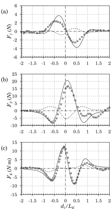
Fig. 6 shows the interactions forces on Model E at Fn=0 passed by Model D at 394
Fn =0.078. In engineering practice, this case study aims to investigate the moor-395
ing forces induced by a passing ship in the harbor areas or inland waterways. 396
Fig. 7 and Fig. 8 shows the interaction forces on Model E at Fn=0.039 and 397
Fn=0.078 encountered by Model D at Fn=0.078. These two case studies aim to 398
validate the feasibility of the present superposition method on simulating the 399
ships moving towards opposite directions. Fig. 9 shows the interactions forces 400
on Model E at Fn=0.078 overtaken by Model D at Fn =0.117. In all of these four 401
cases, the forces on both ships are calculated numerically. However, only the 402
forces on Model E, which was towed by the main carriage, were measured in 403
model tests. Generally, the agreement between present potential flow solver 404
(MHydro) and experimental measurement is very good. It indicates the poten-405
tial flow method is applicable to predict the hydrodynamic interactions between 406
two ships with different forward speeds. 407
X
13
It is found from Fig. 6-Fig. 9.(a) that the resistance (F1) is overestimated by the 408
present potential flow solver, even though the viscous effect is not taken into 409
account. It indicates the hydrodynamic interaction force plays a dominate role 410
in total resistance, and the frictional component due to the viscosity is negligi-411
ble. The negative values shown in Fig. 6-Fig. 9.(a) represent the resistance that 412
is opposite to the moving direction, while the positive values represents a thrust 413
which is the same as the moving direction. An interesting finding is that a very 414
large thrust force is observed at dl / LE = -0.5 during the passing and encounter-415
ing maneuvering. Physically it can be explained that before passing and encoun-416
tering (0 < dl / LE < 1), the presence of the other moving vessel stops the water 417
from spreading evenly into the surrounding field. As a result, the pressure dis-418
tributed over ship bow increases. At the same time, the pressure distributed 419
over ship stern retains the same level. An increased resistance is expected by 420
pressure integral. After encountering (-1 < dl / LE < 0), the high pressure area 421
transfers to the ship stern, which will correspondingly lead to a propulsion force. 422
But in overtaking maneuvering shown in Fig. 9.(a), the thrust force is observed 423
at dl / LE = 0.5, where the bow of Model D approaches the midship of Model E 424
longitudinally. It can be explained that before overtaking (-1 < dl / LE < 0), the 425
presence of faster ship (Model D) accelerates the fluid velocity around the stern 426
area of Model E. As a result, the pressure distributed over ship stern decreases. 427
At the same time, the pressure distributed over ship bow retains the same level. 428
An increased resistance is expected by pressure integral over the hull surface of 429
Model E. After overtaking (0 < dl / LE < 1), the high pressure area transfers to 430
the ship bow, which will correspondingly lead to a propulsion force. 431
During the passing, encountering and overtaking process, the symmetry of the 432
flow in the starboard and port side is violated by the presence of the other vessel. 433
The maximum asymmetric flow is observed when the midships of the two ships 434
are aligned (dl / LE ≈ 0, as shown in Fig. 1), and the suction force reaches its peak 435
value (see Fig. 6-Fig. 9.(b)). The pressure distribution is not only asymmetric in 436
port side and starboard, but also in bow and stern. Consequently, a yaw moment 437
will be induced, as shown in Fig. 6-Fig. 9.(c). Generally, there are four peaks of 438
yaw moment during passing and encountering maneuvering, which appear at 439
dl / LE ≈ -0.6, dl / LE ≈ -0.1, dl / LE ≈ 0.4 and dl / LE ≈ 0.9. But in overtaking 440
process, only three peaks are observed at dl / LE ≈ -0.8, dl / LE ≈ -0.1 and dl / LE 441
≈ 0.5. Based on these peaks, some empirical formulas were established to model 442
the interaction moment (Lataire et al., 2012; Vantorre et al., 2002; Varyani et 443
al., 2002). However, as the numbers of the peaks are not predictable, the ap-444
plicability of those empirical formulas is very limited. It should be noted that in 445
ship-bank and ship-lock problem, potential flow method fails to predict the sign 446
of yaw moment due to the weak lifting force caused by the cross-flow in the stern 447
(Yuan and Incecik, 2016a). However, in ship-ship problem, the hydrodynamic 448
interaction is much more important than cross-flow effects. The predictions of 449
yaw moment by a potential flow solver are therefore reliable. 450
It is also found from Fig. 6-Fig. 9 that the interaction forces on the ship with 451
lower speed is larger than that with higher speed. In passing operation (see Fig. 452
6), the hydrodynamic interaction on Model E is significant, even though Model 453
E is stationary without forward speed. On the contrary, the interaction is neg-454
ligible on the moving ship (Model D) during passing operation. It indicates that 455
the slower ship is more likely to lose its maneuverability during passing, en-456
14
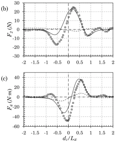
Fig. 6. (a) The resistance, (b) the sway force and (c) the yaw moment on Model E
(j=1) at Fn=0 passed by Model D (j=2) at
Fn =0.078. The positive dl values denote
that Model D is in the upstream side of Model E. As Model D moves to the down-stream side, dl becomes negative. EFD
results are published by Vantorre et al. (2002).
Fig. 7. (a) The resistance, (b) the sway force and (c) the yaw moment on Model E
(j=1) at Fn=0.039 encountered by Model D
(j=2) at Fn =0.078. The positive dl values
denote that Model D is in the upstream side of Model E. As Model D moves to the downstream side, dl becomes negative.
EFD results are published by Vantorre et al. (2002).
458
-6 -4 -2 0 2 4 6
-2 -1.5 -1 -0.5 0 0.5 1 1.5 2
F1
(N
)
E (MHydro) D (MHydro) E (Exp.)
-6 -4 -2 0 2 4 6
-2 -1.5 -1 -0.5 0 0.5 1 1.5 2
F1
(N
)
-10 -5 0 5 10 15 20 25
-2 -1.5 -1 -0.5 0 0.5 1 1.5 2
F2
(N
)
-10 -5 0 5 10 15 20 25
-2 -1.5 -1 -0.5 0 0.5 1 1.5 2
F2
(N
)
-15 -10 -5 0 5 10 15
-2 -1.5 -1 -0.5 0 0.5 1 1.5 2
F6
(N∙m
)
dl/LE
-15 -10 -5 0 5 10 15
-2 -1.5 -1 -0.5 0 0.5 1 1.5 2
F6
(N∙m
)
dl/LE
-6 -4 -2 0 2 4 6
-2 -1.5 -1 -0.5 0 0.5 1 1.5 2
F1
(N
)
E (MHydro) D (MHydro) E (Exp.)
-15 -10 -5 0 5 10 15
-2 -1.5 -1 -0.5 0 0.5 1 1.5 2
F1
(N
)
(a)
(b)
(c)
(a)
(b)
(c)
[image:14.595.316.508.67.425.2] [image:14.595.103.296.71.428.2]15
Fig. 8. (a) The resistance, (b) the sway force and (c) the yaw moment on Model E
(j=1) at Fn=0.078 encountered by Model D
(j=2) at Fn =0.078. The positive dl values
denote that Model D is in the upstream side of Model E. As Model D moves to the downstream side, dl becomes negative.
EFD results are published by Vantorre et al. (2002).
Fig. 9. (a) The resistance, (b) the sway force and (c) the yaw moment on Model E
(j=1) at Fn=0.078 overtaken by Model D
(j=2) at Fn =0.117. The negative dl values
denote that Model D is in the down-stream side of Model E. As Model D moves to the upstream side, dl becomes
positive. EFD results are published by Vantorre et al. (2002).
5 DISCUSSIONS ON FREE-SURFACE EFFECTS
459
The predictions of the yaw moment by a potential-flow solver are therefore reli-460
able. After the aforementioned validations against physical model tests, the pre-461
sent superposition method was extended to investigate the free-surface effects. 462
Here, we study the interactions between two identical Wigley III hulls in head-463
on encounter. The geometry of the hull can be found in Journee (1992). Fig. 10 464
shows the panels distributed on the partial computational domain. The panel 465
number per ship length κ=60. Δt=2t’ is applied in all of the numerical simula-466
tions reported below. We computed the interaction forces in 6DoF (6 Degrees of 467
Freedom), as well as the total wave elevation. 468
469
Fig. 10. Panel distribution on the computational domain of two identical Wigley III 470
hulls in head-on encounter with Fn=0.3, dt/B=2, and dl/L=1. There are 17,760 panels
471
distributed on the entire computational domain: 600 on the wetted body surface of each
472
-30 -20 -10 0 10 20 30
-2 -1.5 -1 -0.5 0 0.5 1 1.5 2
F2
(N
)
-30 -20 -10 0 10 20 30
-2 -1.5 -1 -0.5 0 0.5 1 1.5 2
F2
(N
)
-15 -10 -5 0 5 10 15
-2 -1.5 -1 -0.5 0 0.5 1 1.5 2
F6
(N∙m
)
dl/LE
-60 -40 -20 0 20 40
-2 -1.5 -1 -0.5 0 0.5 1 1.5 2
F6
(N∙m
)
dl/LE
(b)
(c)
(b)
[image:15.595.102.295.71.306.2] [image:15.595.316.507.72.306.2] [image:15.595.145.464.591.724.2]16
hull and 16,560 on the free-surface. The computational domain is truncated at 2L
up-473
stream, 2L downstream and 0.5L laterally with regard to the body-fixed reference
474
frame.
475
5.1 The effect of near-field disturbance and far-field waves 476
Fig. 11 shows the results of the lateral (sway) forces on two identical Wigley III 477
hulls in head-on encounter with dt/B=2. Here we compare the results obtained 478
by using three different methods. In the first method, the encountering problem 479
is treated as a steady problem, although the steady linearized free-surface con-480
dition is applied. Mathematically, in the pressure calculation, the first term in 481
Eq. (27) is neglected. Meanwhile, the first two time-dependent terms in Eq. (16) 482
are also not taken into account. It has been approved to be an efficient method 483
to deal with the steady problems, e.g., interactions between two ships travelling 484
with the same speed (Yuan et al., 2015), or between the hulls of a catamaran or 485
trimaran (Shahjada Tarafder and Suzuki, 2007). In the second method, the en-486
countering is treated as an unsteady problem, while the rigid condition is ap-487
plied on the free-surface. Mathematically, the free-surface condition in Eq. (16) 488
is replaced by an impermeable boundary condition. The BVP therefore is solved 489
as a steady problem. The only unsteady effects are reflected by the time-depend-490
ent term in Eq. (27). Nearly all the published studies on ship-to-ship problem 491
are based on this partially unsteady method (Korsmeyer et al., 1993; Xu et al., 492
2016; Yeung, 1978; Zhou et al., 2012). The advantage of this rigid-free-surface 493
method is obvious. As the image method can be applied on the free-surface, it 494
doesn’t require panels to be distributed on the free surface. It significantly re-495
duces the panel number, herein reducing the calculation time to solve the BVP. 496
However, this method is only applicable when the speed of the ships is low. The 497
third method proposed by the present study takes all the unsteady effects into 498
account. The time derivatives in both Eq. (16) and Eq. (27) are considered. The 499
BVP is solved in the time domain by using an iteration scheme. The advantage 500
of this fully unsteady method is that it can predict the hydrodynamic interaction 501
induced by the ship-generated waves. But the panels must be distributed on the 502
free-surface, which not only increases the total mesh number, but only add dif-503
ficulties to construct the computational domain at each time step. To deal with 504
this issue, we developed a dynamic meshing technique to generate the mesh 505
automatically at each time step. With regard to the computational time, the 506
third method takes longer than the other two methods. But within the frame-507
work of potential flow theory, the computational time is still very satisfactory. 508
Most of the computational efforts are spent on generating the so-called coeffi-509
cient matrix (Hess and Smith, 1964) Even though it involves time iteration, the 510
coefficient matrix retains unchanged. The time scale to solve the unsteady BVP 511
for each time step is few minutes. 512
The results shown in Fig. 11 clearly demonstrate the effects of unsteady pres-513
sure and unsteady free-surface. Here, we note that the unsteady pressure term 514
in Eq. (27) is very important at all the range of encountering speeds, while the 515
free-surface effect is only important when the encounter speed is moderate or 516
high. Ignoring the unsteady pressure term in Eq. (27) will lead to mis-estima-517
tion of the interaction force. At Fn = 0.1, the free-surface elevation and hydrody-518
namic interaction are mainly determined by the near-field (non-wave-like) dis-519
turbances. The rigid free-surface condition (RFC) is adequate to predict the in-520
teraction forces, as shown in Fig. 11(a). As the Froude number increases to Fn 521
=0.2, the far-field waves become manifest, and the interaction force oscillates 522
17
still dominated by the near-field disturbance. The contribution of the force in-524
duced by far-field waves is smaller than that induced by the near-field disturb-525
ance. The fluctuations due to the far-field waves will not deviate from the near-526
field induced forces. The interaction force predicted by rigid free-surface condi-527
tion is symmetric with respect to dl/L=0. But this symmetry property is violated 528
by the presence of the far-field waves. As the far-field waves could not propagate 529
ahead of the ship, the free-surface effect cannot be observed before the encoun-530
tering taken place (dl/L>1). As the encountering ships are maneuvering to each 531
other’s wake region, the free-surface effect then can be observed, and some fluc-532
tuations can be observed at dl/L<1 correspondingly. These fluctuations will not 533
disappear (but the amplitude will decrease) after the encountering operation. 534
The relationship between the near- and far-field induced force is very similar to 535
that between low- and wave-frequency surge or sway motions of a floating struc-536
ture in irregular waves (Yuan et al., 2014a). The free-surface effect becomes 537
even more significant at Fn = 0.3. The force amplitude induced by the far-field 538
waves is larger than that induced by the near-field disturbance, as shown in 539
Fig. 11(c). There are only three peaks induced by near-field disturbance. How-540
ever, the peaks altered by the far-field waves are unpredictable. Therefore, the 541
empirical formulas based on low speed model (Lataire et al., 2012; Vantorre et 542
al., 2002; Varyani et al., 2002) is not applicable to predict the interaction forces 543
when the free-surface effect becomes important. It can be concluded that the 544
free-surface effects must be taken into account at Fn > 0.2. 545
-0.1 -0.05 0 0.05 0.1 0.15
-2 -1 0 1 2
CY
dl/L
Unsteady + LFC Unsteady + RFC Steady + LFC
-0.15 -0.1 -0.05 0 0.05 0.1 0.15
-2 -1 0 1 2
CY
dl/L
λ/L
(a)
18
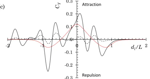
Fig. 11. Sway force acting on two identical Wigley III hulls in head-on encounter with 546
dt/B=2. (a) Fn=0.1; (b) Fn=0.2; (c) Fn=0.3. dl/L=0 corresponds to the moment t=ts, when
547
the midships of the two ships are aligned. dl/L>0 corresponds to t<ts, dl/L<0 corresponds to 548
t>ts. CY is non-dimensionalized by 1
2𝜌𝐵𝑇|𝑈1𝑈2|. LFC indicates that the linearized
free-549
surface condition is used; RFC indicates that the rigid-wall free-surface condition is
550
used.
[image:18.595.189.426.569.695.2]551
Fig. 12 shows the wave profile at the moment when the midships of two Wigley 552
hulls are aligned. The ‘Steady’ indicates the first two terms in Eq. (16) are ig-553
nored, while ‘Unsteady’ indicates the BVP is solved fully in the time domain by 554
using an iteration scheme. At low Froude number Fn=0.1, the unsteady effect 555
on free-surface condition is not essential. As the wave elevation is dominant by 556
the near-field disturbance, the wave-like fluctuations can hardly be observed at 557
low forward speed. At moderate Froude number, the unsteady effect becomes 558
manifest, especially at the gap between two aligned ships (-0.5<x/L>0.5). as the 559
Froude number increases to Fn=0.3, the difference between ‘Steady’ and ‘Un-560
steady’ can be observed in a wider range of x/L, especially at the bow (x/L=0.5) 561
and stern (x/L=-0.5) areas. Fig. 13 shows the wave elevation components ob-562
tained by the present superposition principle. It should be noted that the total 563
wave elevation presented in Fig. 13(c) is not the simple superposition of the 564
waves produced by two individual hulls without considering the presence of the 565
other one. When we calculate the wave elevation produced by B1, the presence 566
of B2 is also considered, treated as an obstacle, by being momentarily stationary 567
in the body-fixed frame of B1. Therefore, the diffraction and reflection by B2 is 568
considered in the present study. These reflected waves can be seen clearly from 569
Fig. 13(a) and (b). 570
571
Fig. 12. Wave profiles at the center line between two identical Wigley III hulls in head-572
on encounter with dt/B=2, dl/L =0 and Fn=0.3. The black, red and blue curves
corre-573
spond to Fn=0.1, 0.2 and 0.3 respectively.
574
-0.3 -0.2 -0.1 0 0.1 0.2 0.3
-2 -1 0 1 2
CY
dl/L
-0.02 -0.01 0 0.01 0.02
-1.5 -1 -0.5 0 0.5 1 1.5
Cζ
x/L
Steady Unsteady
(c) Attraction
19 575
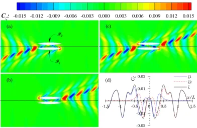
Fig. 13. Waves produced by two Wigley III hulls in head-on encounter with dt/B=2,
576
dl=0 and Fn=0.3. (a)Cζ1, the waves produced by B1 moving at Fn=0.3 while B2is
mo-577
mentarily stationary in the body-fixed frame of B1; (b)Cζ2, the waves produced by B2 578
moving at U2 while B1is momentarily stationary in the body-fixed frame of B2; (c)Cζ,
579
the total waves superposing Cζ1 and Cζ2; (d) Wave profile at the centre line between
580
two hulls shown in (a), (b) and (c).x in the abscissa of (d) refers to the
midship-to-mid-581
ship distance between left-moving ship and the encountered ship.
582
5.2 The effect of divergent and transverse waves 583
Fig. 14 shows the encountering process of two ships in the body-fixed frame of 584
B2. The contour only shows the wave patterns generated by B2 at Fn=0.3 in an 585
unconfined waterway. For a 3D ship, its far-field wave patter includes two wave 586
systems: bow wave and stern wave. Each wave system has two wave compo-587
nents: divergent wave and transverse wave. In the body-fixed frame of B2, B1 588
approaches B2 from its upstream side to its downstream side. Theoretically, B2 589
will experience 6 stages over the entire encountering process: i, non-interference 590
→ ii, local wave disturbance → iii, divergent bow wave disturbance → iv, trans-591
verse bow wave disturbance → v, divergent stern wave disturbance → vi, trans-592
verse wave disturbance. The non-interference stage can only be observed when 593
two ships are sufficient far apart from each other. The transverse bow waves 594
are always interfered with the divergent stern waves. The disturbance in the 595
stage iii, iv and v is supposed to be violate and unpredictable. In the present 596
study, stage iii, iv and v are categorized as a combined stage, namely divergent 597
disturbance. Finally, the interference is divided into three regions: I: t < t1, B1 598
is in the local wave disturbance region of B2; II: t1 < t < t2, B1 is in the divergent 599
wave disturbance region of B2; III: B1 is in the transverse wave disturbance re-600
gion of B2. Here t1 refers to the moment when the bow of B1 reaches the Kelvin 601
envelope of the waves generated by B2, and t2 refers to the moment when the 602
stern of B1 leaves the divergent stern waves generated by B2. 603
C
:
-0.015 -0.012 -0.009 -0.006 -0.003 0.000 0.003 0.006 0.009 0.012 0.015-0.02 -0.01 0 0.01 0.02
-1.5 -1 -0.5 0 0.5 1 1.5
Cζ
x/L
ζ1 ζ2 ζ
(a) (c)
(b) (d)
20 604
Fig. 14. Sketch showing the encountering process of two ships in the body-fixed frame 605
of B2. The bow and stern of the ships act like two sources (or sinks). The blue and red 606
curves represent bow and stern wave patterns respectively.
[image:20.595.167.376.350.680.2]607
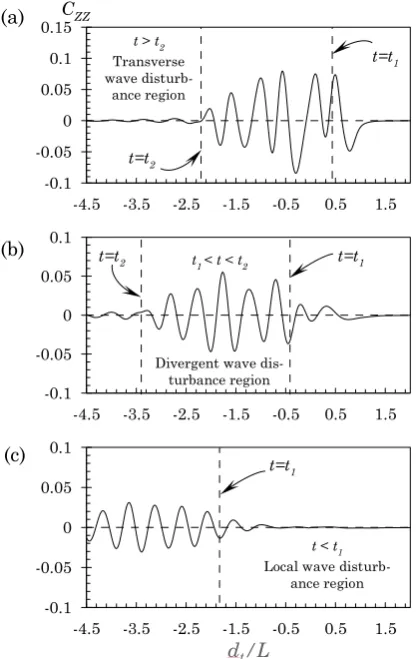
Fig. 15. Yaw moment acting on two identical Wigley III hulls in head-on encounter at
608
Fn=0.3. (a) dt/B=2; (b) dt/B=5; (c) dt/B=10. CZZ is non-dimensionalized by 12𝜌𝐵𝑇𝐿|𝑈1𝑈2|.
609
dl/L>0 corresponds to t<ts, dl/L<0 corresponds to t>ts.
610
Fig. 15 shows the yaw moment on B1 during the encountering process. Different 611
lateral separations are investigated here. As the lateral separation increases, 612
-0.1 -0.05 0 0.05 0.1 0.15
-4.5 -3.5 -2.5 -1.5 -0.5 0.5 1.5
t=t1
t=t2 t > t2 Transverse wave
disturb-ance region
CZZ
-0.1 -0.05 0 0.05 0.1
-4.5 -3.5 -2.5 -1.5 -0.5 0.5 1.5
t=t1
Divergent wave dis-turbance region t=t2 t1 < t < t2
-0.1 -0.05 0 0.05 0.1
-4.5 -3.5 -2.5 -1.5 -0.5 0.5 1.5
dt/L
t=t1
t < t1 Local wave
disturb-ance region U2
U1 Diverging waves
Transverse waves
t < t1 Local wave dis-turbance region
t1 < t < t2 Divergent wave disturbance region
t > t2 Transverse wave disturbance region
t=t1 t=t2
B1 B2
(a)
(b)
21
the non-interference region expands and the disturbance region shifts down-613
stream with regards to the body-fixed frame of B2. It agrees with the physical 614
observation of the far-field waves (Kelvin waves) that confines within Kelvin 615
wedge downstream. Before B1 reaches the Kelvin envelope, some interactions 616
are observed at t < t1, which is due to the disturbance caused by the local waves. 617
The typical wave patterns at t < t1 is shown in Fig. 16(a). At t = t1, when the bow 618
of B1 is stroken by the divergent waves produced by B2, a very large yaw moment 619
can be induced. When B1 is partly or completely in the divergent disturbance 620
region (t1 < t < t2), the interaction becomes significant. The bow and stern waves 621
interfere in this region, and the wave energy concetrated in this region is 622
usually high, especially when the ship speed is moderate or high. The typical 623
wave patterns at t1 < t < t2 is shown in Fig. 16(b). When B1 completely leaves the 624
divergent disturbance region and enters into the transverse disturbance region 625
(t > t2), the amplitude of the interaction force decreases with the decay of the 626
transverse waves. The typical wave patterns at t > t2 is shown in Fig. 16(c). It 627
should be noted that at dt/B=10, the forces at the moment t = t2 is not captured 628
in Fig. 15(c). As the lateral separation increases, t2 will shift further 629
downstream. Numerically, to simulate the case with larger lateral separation, 630
the computational domain must be expanded not only to the lateral sides, but 631
also to the downstream direction. Much more computational efforts are required 632
to simulate the entire encountering process when the lateral separation 633
becomes large. It can also be found from Fig. 15 that as the lateral separation 634
increases, the interaction diminishes, but not significantly. The maximum yaw 635
moment at dt/B=10 still accounts for 40% of that at dt/B=2. It indicates that 636
the hydrodynamic interaction induced by the far-field waves is very important 637
at moderate or high speed encountering operation. It must be taken into account 638
even though the lateral separation between ships is large. 639
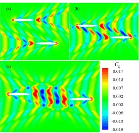
[image:21.595.167.443.440.703.2]640
Fig. 16. Wave patterns produced by two identical Wigley III hulls in head-on encounter 641
at Fn=0.3. (a) dt/B =10 and dl/L= -1, corresponding to t < t1 when a ship is in the other
642
ship’s local wave disturbance region; (b) dt/B =5 and dl/L = -1.5, corresponding to t1 < t
643
< t2 when a ship is in the other ship’s divergent wave disturbance region; (a) dt/B=2 and
644
C 0.017 0.012
0.007
0.002 -0.003
-0.008
-0.013 -0.018
(a) (b)
22
dl/L = -2.5, corresponding to t > t2 when a ship is in the other ship’s transverse wave
645
disturbance region.
646
6 CONCLUSIONS
647
A linearized free-surface boundary condition was used to solve the BVP involved 648
in multiple bodies travelling with various speeds. Based on superposition prin-649
cipal, the traditional coupled BVP could be decoupled into N (assuming there 650
are N bodies) sets of independent unsteady BVPs, which can be solved individ-651
ually in time domain. The advantage of this decoupled method is that the free-652
surface boundary condition can be taken into consideration for each set of inde-653
pendent BVPs. Thus, the unsteady hydrodynamic interaction problem can be 654
solved in a fully unsteady manner, and the far-field wave effect can be can be 655
accounted for. 656
The present formulation provides an effective way to predict the free-surface 657
effects, with particular application for calculating the lateral interaction force 658
on arbitrary number of ships, each with its own speed. By integrating the pre-659
sent superposition method into a Rankine source (simple-source) panel code, we 660
calculated the unsteady hydrodynamic interaction forces and wave elevation 661
when two ships were under passing, overtaking and encountering operations. 662
Experimental measurements confirm the applicability of the present approach. 663
Numerical results indicate the near-field disturbances are the most important 664
component of the interaction force when the encountering speed is low. As the 665
encountering speed increases, the interaction force induced by the far-field 666
waves becomes manifest gradually. It was found the free-surface effects must 667
be considered at Fn > 0.2 for slender ships. For blunt-body ships, the lower limit 668
of Froude number is smaller. When the encountering speed reaches Fn = 0.3, 669
the free-surface effect becomes the dominant component. The interaction force 670
induced by the divergent waves could reach a very large value, which may cause 671
ship accidents, such as grounding, capsizing or collisions. By increasing the sep-672
aration distance between encountering ships could reduce the interaction am-673
plitude, but not significantly. At high encountering speed, the free-surface must 674
be taken into account even though the lateral separation between ships is large. 675
The superposition method proposed in the present study is not limited to 676
solving the unsteady interaction problem between ships. It can also be applied 677
to predict the hydrodynamic interactions between competitive swimmers in a 678
swimming pool, or between aquatic animals swimming near the free surface. 679
The present approach provides a rational and rapid (real-time level) tool for 680
analyzing and computing interaction effects, without going through a lengthy 681
detailed CFD type computations, which would be prohibitively slow (e.g., Zou 682
and Larsson (2013a)) and have yet reached a state to effectively model unsteady 683
multi-body interaction. 684
7 ACKNOWLEDGEMENTS
685
The first author acknowledges the financially support by a Sir David Anderson 686
Award for his visit to UC Berkeley during which this work was formulated. The 687
third author acknowledges partial support of the American Bureau of Shipping 688
via an endowed chair in Ocean Engineering at UC Berkeley. Discussions with 689
Dr. Lu Wang and Mr. Dongchi Yu of UC Berkeley during the course of this work 690