Extensions of the theory of tent spaces and applications to boundary value problems

(1)

Extensions of the theory of tent spaces

and applications to boundary value

problems

Alex Amenta

June 2016

A thesis submitted for the degree of Doctor of Philosophy of the Australian National University

(2)

(3)

Declaration

I hereby declare that the material in this thesis is my own original work except where stated otherwise.

Part I of this thesis consists of work that has either been published or has been submitted for publication. Chapter 1 has been published as ‘Tent spaces over metric measure spaces under doubling and related assumptions’ in the con-ference proceedings Operator theory in harmonic and non-commutative analysis [3]. Chapter2 is joint work with Mikko Kemppainen, and has been published as ‘Non-uniformly local tent spaces’ in Publicacions Matemàtiques [5]. Chapter 3

has been submitted for publication under the title ‘Interpolation and embeddings of weighted tent spaces’, and is available as an arXiv preprint [4].

PartII will be submitted for publication, pending further additions and mod-ifications.

(4)

(5)

Acknowledgements

I would like to thank my supervisors, Pierre Portal (without whom this thesis would never have been started), and Pascal Auscher (without whom it would never have been finished). It has been an absolute pleasure to work with them, and I look forward to continuing our collaboration. I would also like to thank my honours supervisor, Bryan Wang, for (unintentionally) introducing me to research in analysis. I hope his influence is visible in this work, even 3.5 years after my time with him.

I realise as I write these acknowledgements that there is no way to thank all the friends who have helped me through this thesis—who truly deserve to be thanked individually—without forgetting anybody. Therefore, I thank them all not by name, but with the knowledge that they know who they are.

I thank my collaborators for their high-level distraction: Lashi Bandara, Mikko Kemppainen (whose work I have the honour of including in my thesis), and Jonas Teuwen (whose thesis I have the honour of my work being included in). I also thank my mathematical brothers and sisters: Li Chen, Angus Griffith, Yi Huang, and Sebastian Stahlhut (and also Moritz Egert and Dorothee Frey, although they don’t really fit into this category) for all kinds of mathematical and personal support.

I also thank Vincent, Lila, and Céleste, who were ideal housemates while the most difficult parts of this thesis were being completed.

I thank Ping for her support and for suggesting notation for the real inter-polants of weighted tent spaces.

(6)

(7)

...there is a sort of magic in the written word. The idea acquires substance by taking on a visible nature, and then stands in the way of its own clarification.

W. Somerset Maugham, The Summing Up

tout juste un peu de bruit pour combler le silence tout juste un peu de bruit et rien de plus

(8)

(9)

Abstract

We extend the theory of tent spaces from Euclidean spaces to various types of metric measure spaces. For doubling spaces we show that the usual ‘global’ theory remains valid, and for ‘non-uniformly locally doubling’ spaces (including

Rn with the Gaussian measure) we establish a satisfactory local theory. In the

doubling context we show that Hardy–Littlewood–Sobolev-type embeddings hold in the scale of weighted tent spaces, and in the special case of unbounded AD-regular metric measure spaces we identify the real interpolants (the ‘Z-spaces’) of weighted tent spaces.

Weighted tent spaces andZ-spaces on_Rn_{are used to construct Hardy–Sobolev} and Besov spaces adapted to perturbed Dirac operators. These spaces play a key role in the classification of solutions to first-order Cauchy–Riemann systems (or equivalently, the classification of conormal gradients of solutions to second-order elliptic systems) within weighted tent spaces andZ-spaces. We establish this clas-sification, and as a corollary we obtain a useful characterisation of well-posedness of Regularity and Neumann problems for second-order complex-coefficient ellip-tic systems with boundary data in Hardy–Sobolev and Besov spaces of order

(10)

(11)

Introduction

This thesis consists of two main parts. In the first part we provide various gen-eralisations and extensions of the theory of tent spaces. In the second part we establish results concerning the well-posedness of certain elliptic boundary value problems, using some of our extended tent space theory in the process.

Part

I

: Extensions of the theory of tent spaces

Tent spaces were first introduced by Coifman, Meyer, and Stein [32, 33] as a unification of fundamental ideas in modern harmonic analysis. Each of the three chapters of this part provides a different extension of their theory.

Chapter 1: Tent spaces over metric measure spaces under doubling and related assumptions.

The main focus here is on doubling metric measure spaces (X, d, µ): (X, d) is a metric space, µis a Borel measure on (X, d), and the doubling condition

µ(B(x,2r))_.µ(B(x, r)) (x∈X, r >0)

is satisfied. We define tent spaces Tp,q,α(X) associated with such a doubling metric measure space, and establish properties of Tp,q,α(X) analogous to those established by Coifman, Meyer, and Stein in the case where X is _Rn_, _d _{is the} Euclidean distance, and µis the Lebesgue measure.

(16)

The prototypical example of a doubling metric measure space is the Euclidean space_Rnwith the Euclidean distance and Lebesgue measure. More generally, one can consider a Riemannian manifold of non-negative Ricci curvature, equipped with the geodesic distance and Riemannian volume (the curvature assumption ensures that the doubling condition is satisfied, by the Bishop–Gromov compar-ison theorem). Tent spaces associated with doubling Riemannian manifolds are the foundation for the Hardy spaces of differential forms developed by Auscher, McIntosh, and Russ [13] (see also the more recent work on this topic by Auscher, McIntosh, and Morris [11]). However, full details of this tent space theory had not appeared in the literature (with the exception of the atomic decomposition theorem, which was proven explicitly by Russ [81]). Therefore the material of this chapter fills a gap which was perhaps neglected in the past.

Chapter 2: Non-uniformly local tent spaces.

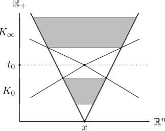
In this chapter we consider metric measure spaces (X, d, γ) which are not bling, but which are—in a certain quantified and non-uniform sense—locally dou-bling (for the precise definition see Section2.2). Given such a space, we construct non-uniformly localtent spacestp,q

α (γ).1 The main difference between these spaces and those constructed in Chapter 1 is that instead of the full ‘upper half-space’

X × _R+, we use an admissible region D ⊂ X × R+ defined in terms of the

‘non-uniform local doubling’ data (see Definition 2.3.1).

Our theory of non-uniformly local tent spaces runs parallel to the theory con-structed in Chapter1. We also prove an atomic decomposition theorem (Theorem

2.4.5). Technicalities imposed on us by the non-uniform local doubling assump-tion force us to require that the metric space (X, d) is complete in the proof of this theorem.

The model non-uniformly locally doubling metric measure space is the Eu-clidean space _Rn _{equipped with the Euclidean distance and, in place of the} Lebesgue measure, theGaussian measure

dγ(x) = 1 (2π)n/2e

−|x|2_/₂ dx.

Non-uniformly local tent spaces associated with this space correspond to the Gaussian tent spaces defined by Maas, van Neerven, and Portal [63]. These are used in the construction of Gaussian Hardy spaces by Portal [78]. In Examples 1_{Note that the notation has changed from the first article: such notation changes will occur}

(17)

2.2.2and2.2.4we provide many other examples of non-uniformly locally doubling spaces, given by weighted measures analogous to the Gaussian measure.

Chapter 3: Interpolation and embeddings of weighted tent spaces. Here we return to the setting of doubling metric measure spaces (X, d, µ) as in Chapter 1. The tent space scale Tp,q₍_X_{) introduced there (we need not make} reference to the aperture parameter α, as we have already shown the tent spaces do not depend on it) is expanded: we define weighted tent spaces Tp,q

s (X) anal-ogously to the spaces Tp,q₍_X_{) =}_Tp,q

0 (X), the difference being the presence of a

weight µ(B(x, t))−s _{in the norm. This is motivated by applications to boundary} value problems (which appear in Part II), where it is often natural to measure the function (t, x)7→t−s_∇_u₍_{t, x}_{) in}_Tp,2₍

Rn) when u is the solution to an elliptic

PDE.

The weighted tent space scale satisfies the following embedding property: when the parameters p0, p1, s0, s1 satisfy the relation2

s1−s0 =

1

p1

− 1

p0

,

we have a continuous embedding

Tp0,q

s0 (X),→T

p1,q

s1 (X)

(Theorem 3.3.19). These embeddings are actually quite counterintuitive. For homogeneous Sobolev spaces a similar embedding property (related to the Hardy– Littlewood–Sobolev lemma) holds, but this is interpreted as an interchange of regularity for integrability. In the context of weighted tent spaces, the parameter

s does not actually reflect any kind of regularity.

When X is unbounded and AD-regular, so that in particular we have

µ(B(x, r))'rn (x∈X, r >0) for some n >0, we identify the real interpolation spaces

(Tp0,q

s0 (X), T

p1,q

s1 (X))θ,pθ =Z

pθ,q

sθ (X) (1)

when p0, p1, q > 1 (Theorem 3.3.4; see Definition 3.3.3 for the definition of the

spaces Zp,q

s (X)). When X = Rn we extend this result to p0, p1 > 0 (Theorem

2_{Normally a factor of some ‘dimension’} _n _{should appear on the right hand side, but this}

(18)

3.3.9). The ‘Z-spaces’Z_sp,q(X) are defined in terms of weightedLp(X×_R+)-norms

of Lq Whitney averages. They have appeared in the work of Barton and May-boroda on elliptic boundary value problems with data in Besov spaces [21], but this connection with weighted tent spaces is new. Furthermore, this shows that Whitney averages arise naturally from the consideration of tent spaces, whereas in the past their use had always been justified by applications to PDE.

Part

II

: Abstract Hardy–Sobolev and Besov spaces for

el-liptic boundary value problems with complex

L

∞

coeffi-cients.

This part of the thesis, unlike the previous part, consists of one single (long) article. Broadly speaking, in this article we construct abstract Hardy–Sobolev and Besov spaces associated with perturbed Dirac operators, and we apply these spaces to the classification of solutions to Cauchy–Riemann systems. The foun-dation for our abstract Hardy–Sobolev and Besov spaces is the theory of weighted tent spaces (and their real interpolants, the Z-spaces) introduced in Chapter 3.

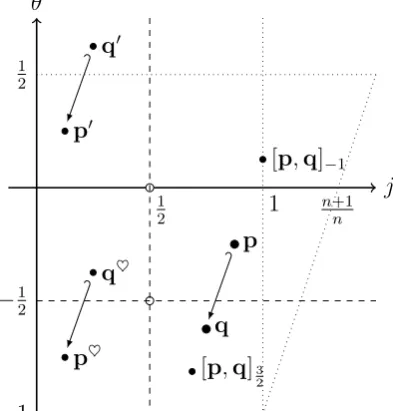
The main trajectory of this article follows the recent works of Auscher and Stahlhut [16] and Auscher and Mourgoglou [14]. However, we introduce many new techniques and shed some additional light on their results. For example, we introduce a new ‘exponent notation’, where boldface letters p are used to denote pairs (p, s) or triples (∞, s;α). The purpose of this notation is to combine integrability and regularity, and in turn to make the exponent calculations used in embeddings and interpolation more intuitive. We also refer to tent spacesTp

s and

Z-spacesZp

s simply asXp, in order to emphasise the fact that these spaces behave in essentially identical ways. This allows us to streamline our proofs, to handle spaces Tp

s and T

∞

s;α on an equal footing, and to prove results for Hardy–Sobolev and Besov spaces simultaneously.

A much more detailed overview of the article is contained in the introduction given there (Chapter 4).

The structure of the thesis

(19)

(20)

(21)

Part I

Extensions of the theory of tent

(22)

(23)

Chapter 1 Tent spaces over metric measure

spaces under doubling and

related assumptions

Abstract

In this article, we define the Coifman–Meyer–Stein tent spaces Tp,q,α(X) asso-ciated with an arbitrary metric measure space (X, d, µ) under minimal geomet-ric assumptions. While gradually strengthening our geometgeomet-ric assumptions, we prove duality, interpolation, and change of aperture theorems for the tent spaces. Because of the inherent technicalities in dealing with abstract metric measure spaces, most proofs are presented in full detail.

1.1 Introduction

The purpose of this article is to indicate how the theory of tent spaces, as devel-oped by Coifman, Meyer, and Stein for Euclidean space in [33], can be extended to more general metric measure spaces. Let X denote the metric measure space under consideration. If X is doubling, then the methods of [33] seem at first to carry over without much modification. However, there are some technicalities to be considered, even in this context. This is already apparent in the proof of the atomic decomposition given in [81].

(24)

— but these proofs are given in the Euclidean context, and no indication is given of their general applicability. In fact, the methods of [44] and [23] can be used to obtain a partial interpolation result under weaker assumptions than doubling. This result relies on some tent space duality; we show in Section 1.3.2 that this holds once we assume that the uncentred Hardy–Littlewood maximal operator is of strong type (r, r) for all r >1.1

Finally, we consider the problem of proving the change of aperture result when

X is doubling. The proof in [33] implicitly uses a geometric property of X which we term (NI), or ‘nice intersections’. This property is independent of doubling, but holds for many doubling spaces which appear in applications — in particular, all complete Riemannian manifolds have ‘nice intersections’. We provide a proof which does not require this assumption.

Acknowledgements

We thank Pierre Portal and Pascal Auscher for their comments and suggestions, particularly regarding the proofs of Lemmas 1.3.3 and 1.4.6. We further thank Lashi Bandara, Li Chen, Mikko Kemppainen and Yi Huang for discussions on this work, as well as the participants of the Workshop in Harmonic Analysis and Geometry at the Australian National University for their interest and suggestions. Finally, we thank the referee for their detailed comments.

1.2 Spatial assumptions

Throughout this article, we implicitly assume that (X, d, µ) is a metric measure space; that is, (X, d) is a metric space and µis a Borel measure on X. The ball centred atx∈X of radius r >0 is the set

B(x, r) :={y∈X :d(x, y)< r},

and we write V(x, r) := µ(B(x, r)) for the volume of this set. We assume that the volume function V(x, r) is finite2 _{and positive; one can show that} _V _is

auto-matically measurable on X×_R+.

There are four geometric assumptions which we isolate for future reference: 1_{This fact is already implicit in [}₃₃_].

(25)

(Proper) a subsetS ⊂Xis compact if and only if it is both closed and bounded, and the volume function V(x, r) is lower semicontinuous as a function of (x, r);3

(HL) the uncentred Hardy–Littlewood maximal operator M, defined for mea-surable functions f onX by

M(f)(x) := sup B3x

1

µ(B)

ˆ

B

|f(y)|dµ(y) (1.1)

where the supremum is taken over all ballsB containingx, is of strong type (r, r) for all r >1;

(Doubling) there exists a constant C >0 such that for all x∈X and r >0,

V(x,2r)≤CV(x, r);

(NI) for all α, β > 0 there exists a positive constant cα,β > 0 such that for all

r >0 and for all x, y ∈X with d(x, y)< αr,

µ(B(x, αr)∩B(y, βr))

V(x, αr) ≥cα,β.

We do not assume that X satisfies any of these assumptions unless mentioned otherwise. However, readers are advised to take (X, d, µ) to be a complete Rie-mannian manifold with its geodesic distance and RieRie-mannian volume if they are not interested in such technicalities.

It is well-known that doubling implies (HL). However, the converse is not true. See for example [37] and [82], where it is shown that (HL) is true for _R2

with the Gaussian measure. We will only consider (NI) along with doubling, so we remark that doubling does not imply (NI): one can see this by taking

R2 (now with Lebesgue measure) and removing an open strip.4 One can show

that all complete doubling length spaces—in particular, all complete doubling Riemannian manifolds—satisfy (NI).

3_{Note that this is a strengthening of the usual definition of a proper metric space, as the}

usual definition does not involve a measure. We have abused notation by using the word ‘proper’ in this way, as it is convenient in this context.

4_{One could instead remove an open bounded region with sufficiently regular boundary, for}

(26)

1.3 The basic tent space theory

1.3.1 Initial definitions and consequences

LetX+_{denote the ‘upper half-space’}_X_×

R+, equipped with the product measure

dµ(y)dt/t and the product topology. Since X and _R+ are metric spaces, with

R+ separable, the Borel σ-algebra on X+ is equal to the product of the Borel

σ-algebras on X and _R+, and so the product measure on X+ is Borel (see [26,

Lemma 6.4.2(i)]).

We say that a subset C ⊂ X+ _is _cylindrical _{if it is contained in a cylinder:}

that is, if there exists x ∈ X and a, b, r > 0 such that C ⊂ B(x, r)×(a, b). Note that cylindricity is equivalent to boundedness when X+ _{is equipped with}

an appropriate metric, and that compact subsets of X+ _{are cylindrical.}

Cones and tents are defined as usual: for each x∈X and α > 0, the cone of aperture α with vertex x is the set

Γα(x) :={(y, t)∈X+ :y∈B(x, αt)}.

For any subset F ⊂X we write

Γα(F) := [ x∈F

Γα(x).

For any subset O⊂X, the tent of aperture α over O is defined to be the set

Tα(O) := (Γα(Oc))c.

Writing

FO(y, t) :=

dist(y, Oc)

t =t

−1

inf

x∈Ocd(y, x),

one can check that Tα(O) = F_O−1([α,∞)). Since FO is continuous (due to the continuity of dist(·, Oc)), we find that tents are measurable, and so it follows that cones are also measurable.

Let F ⊂ X be such that O := Fc has finite measure. Given γ ∈ (0,1), we say that a point x ∈ X has global γ-density with respect to F if for all balls B

containingx,

µ(B∩F)

µ(B) ≥γ.

We denote the set of all such points byF_γ∗, and defineO_γ∗ := (F_γ∗)c_{. An important} fact here is the equality

(27)

where 1O is the indicator function of O. We emphasise that M denotes the uncentred maximal operator. WhenO is open (i.e. whenF is closed), this shows that O ⊂ O_γ∗ and hence that F_γ∗ ⊂ F. Furthermore, the function M(1O) is lower semicontinuous whenever 1O is locally integrable (which is always true, since we assumed O has finite measure), which implies that F_γ∗ is closed (hence measurable) and that O∗_γ is open (hence also measurable). Note that if X is doubling, then since M is of weak-type (1,1), we have that

µ(O_γ∗)_.γ,X µ(O).

Remark 1.3.1. In our definition of points of γ-density, we used balls containing

x rather than balls centred at x (as is usually done). This is done in order to avoid using the centred maximal function, which may not be measurable without assuming continuity of the volume function V(x, r).

Here we find it convenient to introduce the notion of the α-shadow of a subset of X+_{. For a subset}_C _⊂_X+_{, we define the}_α_{-shadow of}_C _{to be the set}

Sα(C) := {x∈X : Γα(x)∩C6=_∅}.

Shadows are always open, for if A ⊂ X+ _{is any subset, and if} _x _∈ _Sα₍_A_), then there exists a point (z, tz) ∈ Γα(x) ∩ A, and one can easily show that

B(x, αtz−d(x, z)) is contained in Sα(A).

The starting point of the tent space theory is the definition of the operators

Aα

q andCqα. Forq∈(0,∞), the former is usually defined for measurable functions

f on_Rn₊+1 (with values in _R or_C, depending on context) by

Aα_q(f)(x)q :=

¨

Γα₍_x₎

|f(y, t)|qdλ(y)dt

tn+1

where x ∈ _Rn _and _λ _{is Lebesgue measure. There are four reasonable ways to} generalise this definition to our possibly non-doubling metric measure space X:5

these take the form

Aα q(f)(x)

q _:=

¨

Γα₍_x₎

|f(y, t)|q dµ(y)

V(a,bt)

dt t

wherea∈ {x, y}andb ∈ {1, α}. In all of these definitions, if a function f onX+

is supported on a subset C ⊂ X+, then Aα

q(f) is supported on Sα(C); we will use this fact repeatedly in what follows. Measurability of Aα

(28)

a=y follows from Lemma1.4.6 in the Appendix; the choicea =x can be taken care of with a straightforward modification of this lemma. The choice a = x, b= 1 appears in [13,81], and the choicea=y, b= 1 appears in [63, §3]. These definitions all lead to equivalent tent spaces when X is doubling. We will take a=y,b=αin our definition, as it leads to the following fundamental technique, which works with no geometric assumptions on X.

Lemma 1.3.2 (Averaging trick). Let α > 0, and suppose Φ is a nonnegative measurable function on X+. Then

ˆ

X

¨

Γα₍_x₎

Φ(y, t) dµ(y)

V(y, αt)

dt

t dµ(x) =

¨

X+

Φ(y, t)dµ(y)dt

t .

Proof. This is a straightforward application of Fubini–Tonelli’s theorem, which we present explicitly due to its importance in what follows:

ˆ

X

¨

Γα₍_x₎

Φ(y, t) dµ(y)

V(y, αt)

dt t dµ(x)

= ˆ X ˆ ∞ 0 ˆ X

1B(x,αt)(y)Φ(y, t)

dµ(y)

V(y, αt)

dt t dµ(x)

= ˆ ∞ 0 ˆ X ˆ X

1B(y,αt)(x)dµ(x) Φ(y, t)

dµ(y)

V(y, αt)

dt t = ˆ ∞ 0 ˆ X

V(y, αt)

V(y, αt)Φ(y, t)dµ(y)

dt t

=

¨

X+

Φ(y, t)dµ(y)dt

t .

We will also need the following lemma in order to prove that our tent spaces are complete. Here we need to make some geometric assumptions.

Lemma 1.3.3. Let X be proper or doubling. Let p, q, α > 0, let K ⊂ X+ be

cylindrical, and suppose f is a measurable function on X+. Then

A α q(1Kf)

_Lp₍_X₎.||f||Lq(K) .

A α q(f)

_Lp₍_X₎, (1.2)

with implicit constants depending on p, q, α, and K.

Proof. Write

(29)

for some x ∈ X and a, b, r > 0. We claim that there exist constants c0, c1 > 0

such that for all (y, t)∈C,

c0 ≤V(y, αt)≤c1.

If X is proper, this is an immediate consequence of the lower semicontinuity of the ball volume function (recall that we are assuming this whenever we assume

X is proper) and the compactness of the closed cylinder B(x, r)×[a, b]. If X is doubling, then we argue as follows. SinceV(y, αt) is increasing int, we have that

min

(y,t)∈CV(y, αt)≥y∈minB(x,r)V(y, αa)

and

max

(y,t)∈CV(y, αt)≤y∈maxB(x,r)V(y, αb).

By the argument in the proof of Lemma 1.4.4 (in particular, by (1.16)), there exists c0 >0 such that

min

y∈B(x,r)V(y, αa)≥c0.

Furthermore, since

V(y, αb)≤V(x, αb+r) for all y∈B(x, r), we have that

max

y∈B(x,r)V(y, αb)≤V(x, αb+r) =:c1,

proving the claim.

To prove the first estimate of (1.2), write

A

α q(1Kf)

_Lp₍_X₎ =

 

ˆ

Sα₍_K₎

¨

Γα₍_x₎

1K(y, t)|f(y, t)|q

dµ(y)

V(y, αt)

dt t

!p_q

dµ(x)

 

1 p

.c0,q

 

ˆ

Sα₍_K₎

¨

K

|f(y, t)|q_dµ₍_y₎dt

t

!p_q

dµ(x)

 

1 p

.K ||f||Lq₍_K₎.

To prove the second estimate, first choose finitely many points (xn)Nn=1 such

that

B(x, r)⊂

N

[

n=1

(30)

using either compactness of B(x, r) (in the proper case) or doubling.6 Write

Bn :=B(xn, αa/2). We then have

¨

K

|f(y, t)|qdµ(y)dt

t

!1_q

.c1

¨

K N

X

n=1

1Bn(y)|f(y, t)|

q dµ(y)

V(y, αt)

dt t

!1q

.X,q N X n=1 ¨ K

1Bn(y)|f(y, t)|

q dµ(y)

V(y, αt)

dt t

!1_q

.

If x, y ∈Bn, then d(x, y)< αa < αt (since t > a), and so

¨

K

1Bn(y)|f(y, t)|

q dµ(y)

V(y, αt)

dt

t ≤

¨

Γα₍_x₎

|f(y, t)|q dµ(y)

V(y, αt)

dt

t . (1.3)

We then have N

X

n=1

¨

K

1Bn(y)|f(y, t)|

q dµ(y)

V(y, αt)

dt t

!1/q

= N X n=1   ˆ Bn ¨ K

1Bn(y)|f(y, t)|

q dµ(y)

V(y, αt)

dt t

!p/q

dµ(x)

  1/p ≤ N X n=1   ˆ Bn ¨

Γα₍_x₎

|f(y, t)|q dµ(y)

V(y, αt)

dt t

!p/q

dµ(x)

  1/p ≤N max n µ(Bn)

−1/p

 

ˆ

X

¨

Γα₍_x₎

|f(y, t)|q dµ(y)

V(y, αt)

dt t

!p/q

dµ(x)

  1/p .K,p,α A α q(f)

_Lp₍_X₎,

which completes the proof.

As usual, with α >0 andp, q ∈(0,∞), we define the tent space (quasi-)norm of a measurable function f onX+ _by

||f||_Tp,q,α₍_X₎ :=

A α q(f)

_Lp₍_X₎,

and the tent space Tp,q,α₍_X_{) to be the (quasi-)normed vector space consisting of} all such f (defined almost everywhere) for which this quantity is finite.

Remark 1.3.4. One can define the tent space as either a real or complex vector space, according to one’s own preference. We will implicitly work in the complex setting (so our functions will always be _C-valued). Apart from complex interpo-lation, which demands that we consider complex Banach spaces, the difference is immaterial.

6_{In the doubling case, this is a consequence of what is usually called ‘geometric doubling’.}

(31)

Proposition 1.3.5. Let X be proper or doubling. For all p, q, α ∈ (0,∞), the tent space Tp,q,α(X) is complete and contains Lq_c(X+) (the space of functions

f ∈Lq(X+) with cylindrical support) as a dense subspace. Proof. Let (fn)n∈N be a Cauchy sequence in T

p,q,α₍_X_{). Then by Lemma} _1.3.3_, for every cylindrical subsetK ⊂X+the sequence (1Kfn)n∈Nis Cauchy inL

q₍_K_). We thus obtain a limit

fK := lim

n→∞1Kfn ∈L

q (K)

for each K. If K1 and K2 are two cylindrical subsets of X+, then fK1|K1∩K2 = fK2|K1∩K2, so by making use of an increasing sequence {Km}m∈N of cylindrical

subsets of X+ _{whose union is} _X+ _{(for example, we could take} _K

m :=B(x, m)× (1/m, m) for some x∈ X) we obtain a function f ∈Lq_loc(X+_{) with} _f_|

Km =fKm

for each m ∈_N.7 _{This is our candidate limit for the sequence (}_f

n)n∈_N.

To see that f lies in Tp,q,α₍_X_{), write for any}_{m, n}_∈

N

||1Kmf||Tp,q,α₍_X₎ .p,q||1Km(f −fn)||Tp,q,α₍_X₎+||1Kmfn||Tp,q,α₍_X₎ ≤Cp,q,α,X,m||f−fn||_Lq₍_K_m₎+||fn||_Tp,q,α₍_X₎,

the (p, q)-dependence in the first estimate being relevant only for p <1 or q <1, and the second estimate coming from Lemma 1.3.3. Since the sequence (fn)n∈_N

converges to 1Kmf inL

q₍_K

m) and is Cauchy in Tp,q,α(X), we have that

||1Kmf||Tp,q,α₍_X₎.sup

n∈N

||fn||Tp,q,α₍_X₎

uniformly in m. Hence ||f||_Tp,q,α₍_X₎ is finite.

We now claim that for allε >0 there existsm∈_Nsuch that for all sufficiently large n∈_N, we have

1Kmc (fn−f)

_Tp,q,α₍_X₎ ≤ε.

Indeed, since the sequence (fn)n∈N is Cauchy in T

p,q,α₍_X_{), there exists} _N _∈

N

such that for all n, n0 ≥N we have ||fn−fn0||

Tp,q,α₍_X₎ < ε/2. Furthermore, since

lim m→∞

1Kmc(fN −f)

_Tp,q,α₍_X₎ = 0

by the Dominated Convergence Theorem, we can choose m such that

1Kmc(fN −f)

_Tp,q,α₍_X₎< ε/2.

7_{We interpret ‘locally integrable on}_X+_{’ as meaning ‘integrable on all cylinders’, rather than}

(32)

Then for all n ≥N,

1Kmc (fn−f)

_Tp,q,α₍_X₎ .p,q

1Kmc (fn−fN)

_Tp,q,α₍_X₎+

1Kmc(fN −f)

_Tp,q,α₍_X₎ ≤ ||fn−fN||Tp,q,α₍_X₎+

1Kmc(fN −f)

_Tp,q,α₍_X₎

< ε,

proving the claim.

Finally, by the previous remark, for all ε >0 we can find m such that for all sufficiently large n∈_N we have

||fn−f||Tp,q,α₍_X₎ .p,q ||1Km(fn−f)||Tp,q,α₍_X₎+

1Kcm(fn−f)

_Tp,q,α₍_X₎

<||1Km(fn−f)||Tp,q,α₍_X₎+ε ≤C(p, q, α, X, m)||fn−f||Lq₍_K

m)+ε.

Taking the limit of both sides asn→ ∞, we find that limn→∞fn=f inTp,q,α(X), and therefore Tp,q,α₍_X_{) is complete.}

To see that Lq

c(X+) is dense in Tp,q,α(X), simply write f ∈ Tp,q,α(X) as the pointwise limit

f = lim

n→∞1Knf.

By the Dominated Convergence Theorem, this convergence holds in Tp,q,α(X).

We note that Lemma 1.3.2 implies that in the case where p = q, we have

Tp,p,α₍_X_{) =} _Lp₍_X+_{) for all} _{α >}_0.

In the same way as Lemma 1.3.2, we can prove the analogue of [33, Lemma 1].

Lemma 1.3.6 (First integration lemma). For any nonnegative measurable func-tion Φ on X+, with F a measurable subset of X and α >0,

ˆ

F

¨

Γα₍_x₎

Φ(y, t)dµ(y)dt dµ(x)≤

¨

Γα₍_F₎

Φ(y, t)V(y, αt)dµ(y)dt.

Remark 1.3.7. There is one clear disadvantage of our choice of tent space norm: it is no longer clear that

||·||_Tp,q,α₍_X₎ ≤ ||·||_Tp,q,β₍_X₎ (1.4)

when α < β. In fact, this may not even be true for general non-doubling spaces. This is no great loss, since for doubling spaces we can revert to the ‘original’ tent space norm (with a=x and b = 1) at the cost of a constant depending only on

(33)

In order to define the tent spacesT∞,q,α(X), we need to introduce the operator

Cα

q. For measurable functions f onX+, we define

Cα

q(f)(x) := sup B3x

1

µ(B)

¨

Tα₍_B₎

|f(y, t)|q_dµ₍_y₎dt

t

!1_q

,

where the supremum is taken over all balls containing x. Since Cα

q(f) is lower semicontinuous (see Lemma 1.4.7), Cα

q(f) is measurable. For functions f on X+ we define the (quasi-)norm ||·||_T∞,q,α₍_X₎ by

||f||_T∞,q,α₍_X₎ :=

C α q(f)

_L∞₍_X₎,

and the tent space T∞,q,α₍_X_{) as the (quasi-)normed vector space of measurable} functions f on X+_{, defined almost everywhere, for which} _||_f_||

T∞,q,α₍_X₎ is finite.

The proof that T∞,q,α₍_X_{) is a (quasi-)Banach space is similar to that of} Propo-sition 1.3.5 once we have established the following analogue of Lemma1.3.3. Lemma 1.3.8. Let q, α > 0, let K ⊂ X+ be cylindrical, and suppose _f is a

measurable function on X+. Then

||f||_Lq₍_K₎.||f||_T∞,q,α₍_X₎, (1.5)

with implicit constant depending only on α, q, and K (but not otherwise on X).

Furthermore, if X is proper or doubling, then we also have

||1Kf||_T∞,q,α₍_X₎.||f||_Lq₍_K₎,

again with implicit constant depending only on α, q, and K.

Proof. We use Lemma 1.4.4. To prove the first estimate, for each ε > 0 we can choose a ball Bε such that Tα(Bε)⊃K and µ(Bε)< β1(K) +ε. Then

||f||_Lq₍_K₎ ≤

1Tα(Bε)f

_Lq₍_X+₎

=µ(Bε)

1 qµ(B

ε)−

1 q

1Tα(Bε)f

_Lq₍_X+₎ ≤(β1(K) +ε)

! q ||_f||

T∞,q,α₍_X₎.

In the final line we used thatµ(Bε)>0 to conclude that

µ(Bε)−1/q

1Tα(Bε)f

_Lq₍_X+₎

is less than theessential supremum of Cα

(34)

For the second estimate, assuming that X is proper or doubling, observe that

||1Kf||T∞,q,α₍_X₎ ≤ sup

B⊂X 1

µ(B)

¨

Tα₍_B₎_∩_K

|f(y, t)|q_dµ₍_y₎dt

t

!1_q

≤ 1

β0(K)

¨

K

|f(y, t)|q_dµ₍_y₎dt

t

!1_q

=β0(K)

−1 q ||f||

Lq₍_K₎,

completing the proof.

Remark 1.3.9. In this section we did not impose any geometric conditions on our space X besides our standing assumptions on the measure µ and the proper-ness assumption (in the absence of doubling). Thus we have defined the tent space Tp,q,α(X) in considerable generality. However, what we have defined is a global tent space, and so this concept may not be inherently useful when X is non-doubling. Instead, our interest is to determine precisely where geometric assumptions are needed in the tent space theory.

1.3.2 Duality, the vector-valued approach, and complex

interpolation

Midpoint results

The geometric assumption (HL) from Section1.2now comes into play. For r≥0, we denote the Hölder conjugate of r byr0 :=r/(r−1) with r0 =∞ when r= 1. Proposition 1.3.10. Suppose that X is either proper or doubling, and satisfies

assumption (HL). Then for p, q ∈(1,∞) and α >0, the pairing

hf, gi:=

¨

X+

f(y, t)g(y, t)dµ(y)dt

t (f ∈T

p,q,α₍_X₎_{, g}_∈_Tp0_,q0_,α

(X))

realises Tp0,q0,α₍_X₎ _{as the Banach space dual of} _Tp,q,α₍_X₎_{, up to equivalence of} norms.

This is proved in the same way as in [33]. We provide the details in the interest of self-containment.

(35)

In general, suppose f ∈Tp,q,α(X) andg ∈Tp0,q0,α(X). Then by the averaging trick and Hölder’s inequality, we have

|hf, gi| ≤

ˆ

X

¨

Γα₍_x₎

|f(y, t)g(y, t)| dµ(y)

V(y, αt)

dt t dµ(x)

≤

ˆ

X

Aα_q(f)(x)A_qα0(g)(x)dµ(x)

≤ ||f||_Tp,q,α₍_X₎||g||_Tp0,q0,α₍_X₎. (1.6)

Thus every g ∈Tp0,q0,α₍_X_{) induces a bounded linear functional on} _Tp,q,α₍_X_{) via} the pairing h·,·i, and soTp0,q0,α₍_X₎_⊂₍_Tp,q,α₍_X₎₎∗_.

Conversely, suppose ` ∈ (Tp,q,α(X))∗. If K ⊂ X+ _{is cylindrical, then by}

the properness or doubling assumption, we can invoke Lemma 1.3.3 to show that ` induces a bounded linear functional `K ∈ (Lq(K))∗, which can in turn be identified with a function gK ∈ Lq

0

(K). By covering X+ _{with an increasing}

sequence of cylindrical subsets, we thus obtain a functiong ∈Lq_loc0 (X+_{) such that}

g|K =gK for all cylindricalK ⊂X+.

If f ∈Lq(X+) is cylindrically supported, then we have

¨

X+

f(y, t)g(y, t)dµ(y)dt

t =

¨

suppf

f(y, t)gsuppf(y, t)dµ(y)

dt t

=`suppf(f)

=`(f), (1.7)

recalling that f ∈ Tp,q,α₍_X_{) by Lemma} _1.3.3_{. Since the cylindrically supported}

Lq₍_X+_{) functions are dense in} _Tp,q,α₍_X_{), the representation (}_1.7_{) of}_`₍_f_{) in terms} of g is valid for all f ∈ Tp,q,α₍_X_{) by dominated convergence and the inequality} (1.6), provided we show that g is in Tp0,q0,α₍_X_).

Now suppose p < q. We will show that g lies in Tp0,q0,α₍_X_{), thus showing} directly that (Tp,q,α₍_X₎₎∗ _{is contained in} _Tp0,q0,α₍_X_{). It suffices to show this for}

gK, where K ⊂ X+ is an arbitrary cylindrical subset, provided we obtain an estimate which is uniform in K. We estimate

||gK|| q0

Tp0,q0,α₍_X₎ =

A

α q0(g_K)q

0

_Lp0/q0₍_X₎

(36)

Fubini–Tonelli’s theorem,

ˆ

X

Aα

q0(g_K)(x)q 0

ψ(x)dµ(x) =

ˆ

X

¨

X+

1B(y,αt)(x)|gK(y, t)|q

0 dµ(y)

V(y, αt)

dt

t ψ(x)dµ(x)

= ˆ ∞ 0 ˆ X 1

V(y, αt)

ˆ

B(y,αt)

ψ(x)dµ(x)|gK(y, t)|q

0

dµ(y)dt

t

=

¨

X+

Mαtψ(y)|gK(y, t)|q

0

dµ(y)dt

t ,

where Ms is the averaging operator defined for y∈X and s >0 by

Msψ(y) := 1

V(y, s)

ˆ

B(y,s)

ψ(x)dµ(x).

Thus we can write formally

ˆ

X

Aα

q0(g_K)(x)q 0

ψ(x)dµ(x) =hfψ, gKi, (1.8) where we define

fψ(y, t) :=

  

Mαtψ(y)gK(y, t) q0/2

gK(y, t)(q

0_/₂₎₋₁

when gK(y, t)6= 0,

0 when gK(y, t) = 0,

noting thatgK(y, t)(q

0_/₂₎₋₁

is not defined when gK(y, t) = 0 and q0 <2. However, the equality (1.8) is not valid until we show thatfψ lies inTp,q,α(X). To this end, estimate

Aα

q(fψ)≤

¨

Γα₍_x₎

Mαtψ(y)q|gK(y, t)|q(q

0₋₁₎ dµ(y)

V(y, αt)

dt t

!1_q

≤

¨

Γα₍_x₎

Mψ(x)q|gK(y, t)|q

0 dµ(y)

V(y, αt)

dt t

!1_q

=Mψ(x)Aα

q0(g_K)(x)q 0_/q

.

Taking r such that 1/p= 1/r+ 1/(p0/q0)0 _{and using (HL), we then have}

A α q(fψ)

_Lp₍_X₎ ≤

(Mψ)A

α q0(g_K)q

0_/q _Lp₍_X₎ ≤ ||Mψ||_L(p0/q0)0₍_X₎

A α q0(g_K)q

0_/q _Lr₍_X₎

.X ||ψ||L(p0/q0)0₍_X₎

A α q0(g_K)

q0/q Lrq0/q₍_X₎ ≤ A α q0(g_K)

(37)

One can show that rq0/q = p0, and so fψ is in Tp,q,α(X) by Lemma 1.3.3. By (1.8), taking the supremum over all ψ under consideration, we can write

||gK||q

0

Tp0,q0,α₍_X₎≤ ||`|| ||fψ||_Tp,q,α₍_X₎

.X ||`|| ||gK|| q0/q

Tp0,q0,α₍_X₎,

and consequently, using that ||gK||_Tp0,q0,α₍_X₎<∞, ||gK||Tp0,q0,α₍_X₎ .X ||`||.

Since this estimate is independent ofK, we have shown thatg ∈Tp0,q0,α(X), and therefore that (Tp,q,α(X))∗ is contained in Tp0,q0,α(X). This completes the proof when p < q.

To prove the statement for p > q, it suffices to show that the tent space

Tp0,q0,α₍_X_{) is reflexive. Thanks to the Eberlein–˘}_{Smulian theorem (see [}₁_{, Corollary} 1.6.4]), this is equivalent to showing that every bounded sequence in Tp0,q0,α₍_X₎ has a weakly convergent subsequence.

Let {fn}n∈_N be a sequence in Tp

0_,q0_,α

(X) with ||fn||_Tp0,q0,α₍_X₎ ≤ 1 for all n ∈

N. Then by Lemma 1.3.3, for all cylindrical K ⊂ X+ the sequence {fn}n∈_N is

bounded in Lq0₍_K_{), and so by reflexivity of} _Lq0₍_K_{) we can find a subsequence}

{fnj}j∈N which converges weakly inL

q0₍_K_{). We will show that this subsequence} also converges weakly inTp0,q0,α₍_X_).

Let ` ∈(Tp0,q0,α(X))∗_{. Since} _p0 _{< q}0_{, we have already shown that there exists}

a function g ∈Tp,q,α(X) such that `(f) = hf, gi. For every ε > 0, we can find a cylindrical set Kε⊂X+ such that

||g −1Kεg||Tp,q,α₍_X₎ ≤ε.

Thus for all i, j ∈_N and for allε >0 we have

`(fni)−`(fnj) =hfni−fnj,1Kεgi+hfni−fnj, g−1Kεgi ≤ hfni −fnj,1Kεgi

+

||fni||Tp0,q0,α₍_X₎+

fnj

_Tp0,q0,α₍_X₎

||g−1Kεg||Tp,q,α ≤ hfni −fnj,1Kεgi+ 2ε.

As i, j → ∞, the first term on the right hand side above tends to 0, and so we conclude that {fnj}n∈N converges weakly in T

p0_,q0_,α

(38)

Remark 1.3.11. As mentioned earlier, property (HL) is weaker than doubling, but this is still a strong assumption. We note that for Proposition 1.3.10 to hold for a given pair (p, q), the uncentred Hardy–Littlewood maximal operator need only be of strong type ((p0/q0)0,(p0/q0)0). Since (p0/q0)0 is increasing in pand decreasing in q, the condition required on X is stronger as p→1 and q→ ∞.

Given Proposition 1.3.10, we can set up the vector-valued approach to tent spaces (first considered in [44]) using the method of [23]. Fix p ∈ (0,∞), q ∈

(1,∞), and α >0. For simplicity of notation, write

Lq_α(X+) :=Lq X+; dµ(y)

V(y, αt)

dt t

!

.

We define an operator Tα: Tp,q,α(X)→Lp(X;Lqα(X+)) from the tent space into theLq_α(X+)-valuedLpspace onX(see [35, §2] for vector-valued Lebesgue spaces) by setting

Tαf(x)(y, t) :=f(y, t)1Γα₍_x₎(y, t).

One can easily check that

||Tαf||_Lp₍_X_;_Lq

α(X+))=||f||Tp,q,α(X),

and so the tent space Tp,q,α₍_X_{) can be identified with its image under} _T α in the space Lp₍_X_;_Lq

α(X+)), provided that Tαf is indeed a strongly measurable function of x ∈ X. This can be shown for q ∈ (1,∞) by recourse to Pettis’ measurability theorem [35, §2.1, Theorem 2], which reduces the question to that of weak measurability of Tαf. To prove weak measurability, supposeg ∈Lq

0

α(X); then

hTαf(x), gi=

¨

Γα₍_x₎

f(y, t)g(y, t) dµ(y)

V(y, αt)

dt t ,

which is measurable in x by Lemma 1.4.6. Thus Tαf is weakly measurable, and therefore Tαf is strongly measurable as claimed.

Now assume p, q ∈ (1,∞) and consider the operator Πα, sending X+-valued functions on X to_C-valued functions on X+, given by

(ΠαF)(y, t) := 1

V(y, αt)

ˆ

B(y,αt)

F(x)(y, t)dµ(x)

whenever this expression is defined. Using the duality pairing from Proposition

(39)

and G∈Lp0(X;Lq_α0(X+)) we have

hhTαf, Gii=

ˆ

X

¨

X+

Tαf(x)(y, t)G(x)(y, t)

dµ(y)

V(y, αt)

dt t dµ(x)

=

¨

X+

f(y, t)

V(y, αt)

ˆ

X

1B(y,αt)(x)G(x)(y, t)dµ(x)dµ(y)

dt t

=

¨

X+

f(y, t)(ΠαG)(y, t)dµ(y)

dt t

=hhf,ΠαGii. Thus Πα maps Lp

0

(X;Lq0

α(X+)) to Tp

0_,q0_,α

(X), by virtue of being the adjoint of

Tα. Consequently, the operator Pα := TαΠα is bounded from Lp(X;Lqα(X+)) to itself for p, q ∈ (1,∞). A quick computation shows that ΠαTα = I, so that Pα projects Lp₍_X_;_Lq

α(X+)) onto Tα(Tp,q,α(X)). This shows that Tα(Tp,q,α(X)) is a complemented subspace of Lp₍_X_;_Lq

α(X+)). This observation leads to the basic interpolation result for tent spaces. Here [·,·]θ denotes the complex interpolation functor (see [22, Chapter 4]).

Proposition 1.3.12. Suppose that X is either proper or doubling, and satisfies

assumption (HL). Then for p0, p1, q0, and q1 in (1,∞), θ ∈[0,1], and α >0, we

have (up to equivalence of norms)

[Tp0,q0,α₍_X₎_{, T}p1,q1,α₍_X_)]

θ =Tp,q,α(X), where 1/p= (1−θ)/p0+θ/p1 and 1/q = (1−θ)/q0+θ/q1.

Proof. Recall the identification

Tr,s,α(X)∼=TαTr,s,α(X)⊂Lr(X;Lsα(X

+₎₎

for all r ∈(0,∞) and s∈(1,∞). Since [Lp0₍_X_;_Lq0

α(X

+

)), Lp1₍_X_;_Lq1

α(X

+

))]θ =Lp(X; [Lq0

α(X

+

), Lq1

α(X

+

)]θ) =Lp(X;Lq_α(X+))

applying the standard result on interpolation of complemented subspaces with common projections (see [89, Theorem 1.17.1.1]) yields

[Tp0,q0,α₍_X₎_{, T}p1,q1,α₍_X_)]

Extensions of the theory of tent spaces and applications to boundary value problems

Extensions of the theory of tent spaces

and applications to boundary value

problems

Alex Amenta

June 2016

Declaration

Acknowledgements

Contents

I

Extensions of the theory of tent spaces

7

II

Abstract Hardy–Sobolev and Besov spaces

101

Introduction

Part

I

: Extensions of the theory of tent spaces

Part

II

: Abstract Hardy–Sobolev and Besov spaces for

el-liptic boundary value problems with complex

L

coeffi-cients.

The structure of the thesis

Part I

Extensions of the theory of tent

Chapter 1

Tent spaces over metric measure

spaces under doubling and

related assumptions

1.1

Introduction

Acknowledgements

1.2

Spatial assumptions

1.3

The basic tent space theory

1.3.1

Initial definitions and consequences

1.3.2

Duality, the vector-valued approach, and complex

interpolation