The Assessment of Machine Learning Model Performance for Predicting Alluvial Deposits Distribution

(1)

Procedia Computer Science 36 ( 2014 ) 637 – 642

Peer-review under responsibility of scientific committee of Missouri University of Science and Technology doi: 10.1016/j.procs.2014.09.067

ScienceDirect

Complex Adaptive Systems, Publication 4

Cihan H. Dagli, Editor in Chief

Conference Organized by Missouri University of Science and Technology

2014-Philadelphia, PA

The Assessment of Machine Learning Model Performance

for Predicting Alluvial Deposits Distribution

Adamu M. Ibrahim and Brandon Bennett

*

School of Computing University of Leeds, UK

Abstract

This paper discusses the development and evaluation of distribution models for predicting alluvial mineral potential mapping. A number of existing models includes Weight of Evidence, Knowledge-driven Fuzzy, Data-driven Fuzzy, Neural-Network, Bayesian Classifier and Geostatistical Kriging. We offer classification models developed in our laboratory, where point pattern analysis was used to identify presence or absence of a known secondary alluvial (cassiterite) deposits in the Nigerian Younger Granite Region (NYGR) and the model performance assessed. We focused on the training and testing data split using longitudinal spatial data splitting (strips and halves) to ensure predictive attribute's independence. The spatial data split runs counter to the traditional random sample data selection as a procedure for checking overfitting of models mainly due to spatial data autocorrelation. Specifically, we used classification algorithms such as; Naive Bayes, Support Vector Machine, K-Nearest Neighbour, Decision Tree Bagging and Discriminant Analysis algorithms for training and testing. We analysed the model's performance results using model predictive accuracy and ROC curve values in two different approaches that improve spatial data independence among predictive attributes to give a meaningful model performance.

Selection and peer-review under responsibility of scientific committee of Missouri University of Science and Technology.

Keywords:machine learning; classification model; spatial auto correlation; younger granite; alluvial deposit.

1. Introduction

Distributions models are mostly used to predict the presence or absence of target deposits in a given area that has not been surveyed or censused [4]. Alluvial deposit represents a point distribution in a particular region on the map. Known occurrence of a particular set of deposits represented as points are characterised to be dependent variables, which are analysed and explained by the geological, geographic and geospatial data [6]. The distribution pattern of secondary alluvial deposits of tin-ore (alluvial placers) has a non-random distribution. The occurrence of secondary alluvial deposit is a result of the interplay of some geological features caused by the superficial weathering and transportation by river flow of primary deposits from the hard rock source to a point of deposit [5]. The modelling of this process involves the source of the mineral deposits, the means of transportation and the point of deposit. Hence, the spatial association between the occurrence of mineral deposits with certain

* Corresponding author. Tel.: +4447407168697; +44(0)1133431070 fax: +44(0)1133435468.

E-mail address:[email protected]; [email protected]

(2)

geological features and measuring of distances between the point of deposits and geological features will give a good descriptive model of the entire alluvial ore deposit formation for predicting future mineral occurrence. The understanding of spatial distribution pattern is one step towards understanding the relationship between mineral deposit locations and their geological features. Analysis of spatial associations of known particular mineral deposits with certain geological features is very useful in weighing the relative importance of each type of geological feature and their effects on mineral deposits [5]. We present a quantitative and purely data-driven approach to modelling, where evidential weights are quantify with respect to locations of known deposits [1].

Geo-spatial and environmental data are very extensive for global coverage and can allow for predicting even uncensored area. Recently, there is a greater attention in modelling distribution patterns using environmental and geospatial data to make predictions based on the projection of predictive attributes of geological and geographic data from models such as global circulation models [18][28]. A mineral distribution model is a vital tool for identifying potential mining areas for economic value and land management [26][14]. It relates to the fundamental question of discovering new mineral deposits which involve the formation, transportation and deposition [8][13]. Known occurrences points are used as dependent variables in relation to the various environmental and geospatial variables such as climate, land cover, lithology and other spatial components within which they occur. Many authors have noted that distribution models tend to omit geospatial and geological processes interactions that are known to be important, and this brings to bear the fundamental question of how good models can be [2][24]. Box in 1976 claims all models are wrong, but says some are useful, and this brings to bear the quantitative test of model performance rather than merely noting their many shortcomings. The predictive test performance of distribution models in the present day suffer from the results of different approaches and an unclear relationship of performance due to complicating factors such as spatial autocorrelation. Spatial autocorrelation is a phenomenon where the presence of some property in a sampling unit makes its presence in neighboring sampling units more or less likely. An example is the relationship between elevation (distance from the river) and rock types (size).

The objective of this paper is to use machine learning (ML) as a tool for modelling geospatial data by building a model capable of learning patterns in geospatial attributes and making predictions. We will use five classification algorithms such as Naive Bayes (NB), Support Vector Machine (SVM), K-Nearest Neighbour (KNN), Decision Tree Bagging (DTB) and Discriminant Analysis (DA). The five algorithms will be used to build predictive models to select the best-performing model based on predictive accuracy and the receiver operating characteristic (ROC) value. We will also apply four methods of splitting techniques to determine the effect of spatial autocorrelation in data and assess model performance using true independent predictive attributes and identify how distribution model performance influenced the information content of dependent and relative independent data attributes. The five algorithms selected were based on their ability to handle supervised machine learning problems such as the classification of alluvial mineral distribution occurrence (labeled data). A vast aspect of input training and testing data potentially influence the outcome of the model test [4].

2. Background and previous work

Several methods exist for model testing or evaluation. The most common is re-substitution, used to measure the goodness-of-fit

of the model by using same data the model train for [15]. This plan can inform the researcher about the ability of the chosen model to describe the given data, but it says little about the generality or transferability of the model [21] or whether the model can satisfactorily predict from new, independent data. A more widely used approach is to randomly hold-out,leave one out cross validation (LOOCV)or through n-fold cross validationfor model building process and testing of fitted model on this held-out test data (predictions) as shown in Figure 1. This plan can consist of holding out a fixed rate of data only once, or holding out small percentage of the data for testing (not used in the model building and parameterizing process) but rotating the random selection and thus repeating the testing process several times, until each data point was in a test set once, and then averaging over the multiple test results (cross-validation). Splitting the data into training and test data not only gives the impression of the goodness-of-fit of the model to the data but also the capability to predict onto new data and therefore its generality and transferability. In general, cross-validation is a model validation technique for assessing the validity or accuracy of a model in predicting into new area. It explains how the results of a statistical analysis will generalize to an independent data set. We proposed a novel spatially segregated hold-out, in contrast to the random hold-out. A spatially segregated hold-out prevents spatial intermingling of training and test datasets and thus makes it more likely that the two datasets are truly independent [29]. However, where the data have no spatial autocorrelation across the modelling extent then it is the same as random holdout approach, but environmental and geospatial distribution data are virtually always autocorrelated in space, which tends further to complicate the model testing process. Spatial autocorrelation follows Tobler's first law which states that, things closer together are more similar than things further apart [20], resulting in a dependence among locations that decays with distance. Autocorrelation is found in both the independent variables especially in geographical and geospatial data and the dependent variable (the mineral distribution). Spatial autocorrelation of dependent and independent variables may lead to model over-fitting or an inflated test measure [27]. Consequences of spatial autocorrelation, such as an overestimation of degrees of freedom, a resulting underestimation of variance and overestimation of the significance, as well as an influence on variable selection, have been investigated in detail [19][11]. However, the consequence of spatial autocorrelation to a test of the predictive power of a model based on data hold-out techniques has received less attention [4]. Several authors have identified predictive test problem and consequently many studies have been conducted by testing models on a presumed independent data [17][3]. There are three approaches to independent testing data which include: independently collected data, temporally independent data and spatially independent data.

(3)

between training and test data leading to overfitting or overly optimistic model evaluations. The challenges in identifying true model performance in distribution modeling typical of this study only reported a measure of performance for prediction into a new area. As such, it is hard to say whether the distribution models predicting to the new area performed well or not. For example, can we say an Area under ROC curve (AU-ROC) of 0.70 when predicting into a new area performed well? These questions may require some form of systematic inference that will allow the identification of those attributes that contribute to drops in model performance. Here, we consider investigating methods of spatial split in model evaluation in a single study so that a decrease in the determined performance is weighted relatively against the conventional methods. So far no mineral deposit prediction studies have investigated such a comparison. This paper investigates the influence of input data and model testing scheme (re-substitution, random reserved data design and spatially segregated data design) on performance tests of alluvial mineral predictive model. The paper also shows how the testing scheme needs to be matched with the intended purpose of the model to prevent overfitting results.

Previous work employed for predicting alluvial mineral potential deposits focused mainly on model fitting and mapping such as in the expert system named Prospector developed at Stanford Research Institute for evaluating mineral prospects [12]. Duda, for example, used Prospector for combining predictor patterns in the study of the Island Copper deposits in British Columbia, and Campbell [10][5] published the results of applying Prospector to map the potential of Molybdenum deposits in Mt.Tolman area of Washington State. Others are Reddy [25] who used GIS methods to map base metal potential in Manitoba. Yatabe and Febbri, Bonham-Carter [31][5] also did a review of the Prospector. Porwal in 2006 developed some mathematical models for mineral potential mapping and evaluated their performance by comparing predictive accuracy of each model [22]. However, our focus is on the model performance evaluation and assessment using truly independent data sets, to achieve a meaningful model performance by reducing the effect of spatial data autocorrelation.

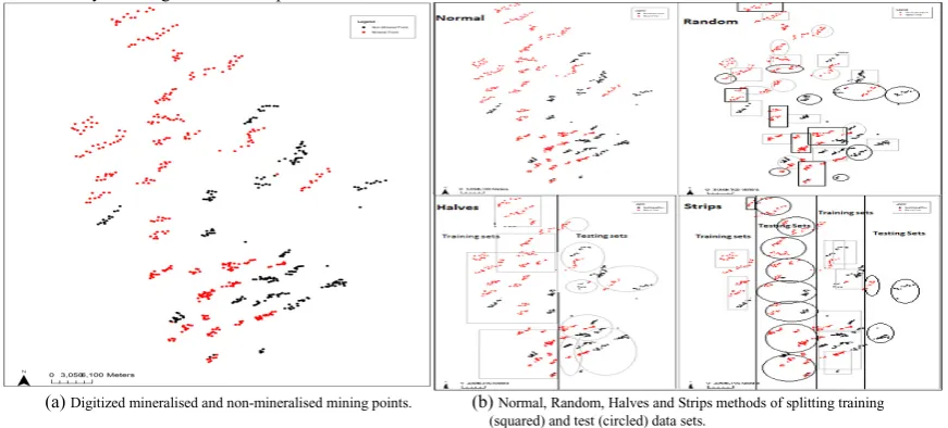
[image:3.544.61.497.256.453.2]

(a) Digitized mineralised and non-mineralised mining points. (b) Normal, Random, Halves and Strips methods of splitting training (squared) and test (circled) data sets.

Fig. 1: Diagrammatical representation of alluvial mineral data points and four way splitting methods of training and testing data in a spatial frame of reference.

3. Study area and data collection.

The Nigeria Younger Granite region (NYGR) constitutes an igneous province which is one of the best examples of mid-plate magmatism in the world, mainly due to the presence of aluminous biotite granites which are the source of rich alluvial tin and columbite [30]. The ring-complexes that formed the province was made of high-level alkaline anorogenic magmatism exposed over a distance of about 200km wide and 1600km long extending from northern Niger down to central Nigeria [7]. The mineral deposits associated with the ring complexes of the province have been the chief motivating force behind geological research in the province, ever since deposits of alluvial tin were first discovered [13]. The alluvial deposits that formed the basis for the Nigerian tin mining industry are mostly secondary mineral that were shaded from the weathering and transportation by river to form cassiterite [30]. More than 98% of the alluvial cassiterite produced from Nigeria was mined in the area around Jos Plateau State and the surrounding NYGR rocks in Bauchi, Nasarawa and Kano states. The area lies between Latitude 9 00'00" N to 10 30'00"N and Longitude 8 30'00"E to 9 30'00"E. We used data from the field survey of all alluvial deposits mining points in Jos-Plateau State area of the NYGR. The survey was conducted for a period of two months by a team of skilled geologist who identified and recorded all present and past mining points. The area is divided into several numbers of mining districts for ease of survey and data collection, each of these districts holds several dozens of mining sites. Data collection sheet was designed to capture the relevant information such as; latitude and longitude, elevation above sea level using Global Positioning System (GPS) equipment while other ancillary information about the mining sites such as sizes, status was established and recorded. Consideration was given to data density as part of sampling values depending on the number of mining sites in a given mining district (i.e. areas with a larger number of mining sites have a denser sampling interval).

4. Methodology

(4)

[image:4.544.163.376.109.278.2]

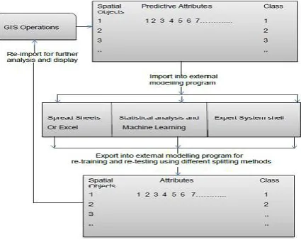
mineral deposits using GIS and machine learning. The figure depicts the process of data analysis (statistical and spatial analysis), visualisation, model building and model evaluation. The model evaluation is the final stage of the diagram and was implemented using the same process as model building but using different splitting approach to input training and testing data as shown in Figure1. The splitting technique is done to achieve data independence and reduce the effect of spatial autocorrelation in the predictive attributes.

Fig. 2: Tabular structure of the methodology adopted for the research.

5. Experimental Data Presentation and Analysis

In Figure 1a, a total number of 690 labelled data points with other predictive attributes are classified as 420 mineralised and 260 non-mineralised points; the mineralised and non-mineralised points classified as binary class indicators of 1 and 0 respectively. Other predictive attributes include map of 15 digitised lithological components of rock types forming 204 polygon units, digital elevation map (SRTM-DEM), the georeferenced TM LANDSAT data map of the area. A spatial analysis using GIS was conducted to measure distances of each mineral and non-mineral points to the nearest rock units and recorded as part of the alluvial mineral predictive attributes. All map layers were carefully overlaid to form a predictive mineral attributes map layers in GIS. The attribute values were extracted from GIS as attribute table representing all data sets in a spatial frame of reference into MATLAB or WEKA for computational modelling (ML). A summary of the list of datasets used for this work indicated in Table 1.

Table 1. Datasets used in the experiment.

Dataset Types Numbers

Mineral Mining Points Points 690

Mineralised mining points Points 460

Non-mineralised mining points Points 240

15 Digitised Rock Layers Polygons 204 Predictive Attributes of points Numeric 24

1965 Map of PYGR Cartographic Map 1

1975 TM-LANDSAT map Landsat map 1

Digitised map of PYGR shape file 1

SRTM DEM Elevation map 1

Mineralised class Binary(0,1) 2

6. Distribution Model Classification and Evaluation

There are available classification algorithms in MATLAB and WEKA. In selecting algorithm to adopt for this work, we consider factors such as the type of data we are dealing with and the techniques that support such type of data. We also consider a trade-off between complexity, restrictiveness in the underlying assumptions associated with certain algorithms and predictive performance of the algorithm. For instance, all the five machine learning algorithms considered for this work, supports labeled data distribution represented as the alluvial mineral data point’s distribution indicating presence and absence of mineral deposit in a given location. We also considered the popularity of such algorithms and their high predictive ability especially NB and DTB that predict very well with both highly correlated and independent data attributes. In general, they all support a supervised machine learning technique.

(5)

strips or (longitudinal) strips worked differently, we first found the 25th, 50th and 75th percentile longitude of all occupied locations and then split the dataset into four parts along these lines, numbered 1 to 4 from west to east. We then used part 1 and 3 combined as training sets and part 2 and 4 as testing sets (see figure 1b). Similarly, for splitting the range in half we found the median longitude of all occupied locations and split the dataset along this longitude. We then used one of the halves to build the models (train set) and the other to evaluate it (test sets). The four different approaches represented a progression from no segregation of training and test data (no spatial split) to a drastic spatial segregation (halves) and then a systematic spatially segregated split between training and test datasets (strips).

7. Discussion and Result Presentation

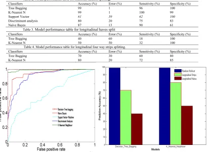
We can see from the results obtained in table 2 that only DTB and KNN performed extremely well (near 100% accuracy). Hence, we will be considering only these two to evaluate their performance using spatial splitting to investigate over-fitting of the model due to spatial autocorrelation associated with predictive spatial data. The DTB training algorithm or sometimes random forests apply the general technique of bootstrap aggregating or bagging to tree learners. Given a training set X = x1……..xnwith responses Y = y1……yn. DTB repeatedly selects a bootstrap sample of the training set and fits trees to these samples, random forest or bootstrap with constant leaf predictors can be interpreted as weighted neighbourhood scheme (KNN algorithm). Bagging was considered as one of the best-modelling technique in terms of predictive power [16][23]. The result of model performance improvement through longitudinal spatial split as an evaluation of the high performing results are obtained in Tables 1 to 4. We also plot the ROC to show the performance of each algorithm in determining how well the models work with TB and KNN which shows some elements of overfitting as shown in Figure 3a.

[image:5.544.73.486.358.659.2]

Our results illustrate how important the selection of a testing scheme is when judging the predictive performance of the distribution model. Doubtlessly, the extremely high measures of performance of Tree bagging (TB) and K-NN as judged by random-hold out testing scheme also indicate overfitting and supplies very similar estimates of performance (see figure 3a). However, TB has been shown to generalize well [9]. The overly optimistic testing results of models with randomly held-out but not fully independent test data is illustrated well by a large drop in performance measures we observed when we tested our models on truly independent, spatially segregated data. The models fared slightly better in the interspersed four-split approach than in the halves approach. The model performance could either be an indication of a remaining effect of autocorrelation along the segregation lines (only one segregation line in the halves approach, but three in the strips approach) or a reduced problem of models predicting into a new area. The significant explanation to the cause of the drop in predictive power of our models when training and test datasets were splitted geographically is the lack of true independent testing data. Hence, we introduced a rather dramatic geographical segregation of the predictive dataset which effectively broke or reduce the dependence due to spatial autocorrelation (see figure 3b).

Table 2. Model performance table for stratified random splitting.

Classifiers Accuracy (%) Error (%) Sensitivity (%) Specificity (%)

Tree Bagging 99 1 96 100

K-Nearest N 99 1 100 99

Support Vector 61 39 62 100

Discriminant analysis 80 20 75 83

Naïve Bayes 87 13 90 61

Table 3.Model performance table for longitudinal haves split

K-Nearest N 50 50 32 100

Table 4. Model performance table for longitudinal four way strips splitting.

K-Nearest N 80 20 72 85

(a) ROC plot for all Classifiers using conventional random hold-out. (b) Assessment of model accuracy using stripping techniques

(6)

8. Conclusion

In conclusion, the research showed that the most widely used and accepted method for testing presence or absence in mineral point distribution models, namely randomly holding out test data led to estimates of high predictive accuracy as well as AUC. The results give a predictive accuracy of 0.99, AU-ROC = 0.99 and accuracy of 0.99, AU-ROC = 0.98 for both TB and K-NN respectively. The result was inflated in comparison to a more rigorous analysis that accounted for the presence of strong autocorrelation in the data as shown in Figure 3 and Tables 3-4, which prevents random hold-out data from being truly independent (even if it was collected independently) and hence causing overfitting. An overfitting creates a false sense of predictive accuracy in model tests. The absence of these more rigorous methods in currently widely used model evaluation practices has far reaching consequences. Evaluation can be achieved through model selection and judging our confidence in the model. Using a testing scheme that leads to overly optimistic evaluations is the case with any test on not entirely independent test data, such an analysis will lead to the selection of overfit models with false insights in which factors are relevant to the distribution model. An overly optimistic and overfit model may lead to false predictions of a given model. Our results suggest that the current opinion about how well distribution models perform may be overly optimistic when extrapolating into new areas or new-geographical regimes for either prediction or understanding, and when testing with interspersed (spatially autocorrelated) data. Distribution modelers should exercise caution when using such models in a predictive fashion, especially under radically changed conditions such as exploring the effects of future geospatial change. The testing scheme used to judge the usefulness of the model needs to match the intended purpose. The proposed model to predict into new areas or conditions will need to be tested using truly independent and spatially segregated data.

References

[1] FP Agterberg, Go F Bonham-Carter, DF Wright, et al. Statistical pattern integration for mineral exploration. Computer applications in estimation prediction and assessment for metals and petroleum, pages 1–21, 1990.

[2] Miguel B Ara´ujo, Richard G Pearson, Wilfried Thuiller, and Markus Erhard. Validation of species–climate impact models under climate Global Change Biology, 11(9):1504–1513, 2005.

[3] Miguel B Ara´ujo and Carsten Rahbek. How does climate change affect biodiversity? SCIENCE-NEW YORK THEN WASHINGTON-, 313(5792):1396, 2006.

[4] Volker Bahn and Brian J. McGill. Testing the predictive performance of distribution models. Oikos, 122(3):321–331, 2013. [5] Graeme Bonham-Carter. Geographic information systems for geoscientists: modelling with GIS, volume 13. Pergamon press, 1994. [6] Barry N Boots and Arthur Getis. Point pattern analysis, volume 10. SAGE publications Newbury Park, CA, 1988.

[7] P Bowden, JN Bennett, Judith A Kinnaird, JE Whitley, SI Abaa, and Penelope K Hadzigeorgiou-Stavrakis. Uranium in the niger-nigeria younger granite province. Mineralogical Magazine, 44(336):379–389, 1981.

[8] P Bowden and JA Jones. Mineralization in the younger granite province of northern nigeria. Metallization Associated with Acid Magmatism, 3:179–190, 1978.

[9] Leo Breiman. Random forests. Machine learning, 45(1):5–32, 2001.

[10] AN Campbell, VF Hollister, RO Duda, and PE Hart. Recognition of a hidden mineral deposit by an artificial intelligence program Science, 217(4563):927–929, 1982.

[11] Mark RT Dale and M-J Fortin. Spatial autocorrelation and statistical tests in ecology. Ecoscience, 9(2):162–167, 2002. [12] Richard O Duda, Peter E Hart, and David G Stork. Pattern classification and scene analysis 2nd ed. 1995.

[13] John Downie Falconer. Nigerian tin; its occurrence and origin. Economic Geology, 7(6):542–546, 1912.

[14] Simon Ferrier. Mapping spatial pattern in biodiversity for regional conservation planning: where to from here? Systematic biology, 51(2):331–363, 2002. [15] Alan H Fielding and John F Bell. A review of methods for the assessment of prediction errors in conservation presence/absence models. Environmental conservation, 24(01):38–49, 1997.

[16] Marta Benito Garzon, Radim Blazek, Markus Neteler, Rut S´anchez de Dios, Helios Sainz Ollero, and Cesare Furlanello. Predicting habitat suitability with machine learning models: The potential area of¡ i¿ pinus sylvestris¡/i¿ l. in the iberian peninsula. ecological modelling, 197(3):383–393, 2006.

[17] Arndt Hampe. Bioclimate envelope models: what they detect and what they hide. Global Ecology and Biogeography, 13(5):469–471, 2004.

[18] Louis R Iverson and Anantha M Prasad. Predicting abundance of 80 tree species following climate change in the eastern united states.Ecological Monographs, 68(4):465–485, 1998.

[19] Pierre Legendre. Spatial autocorrelation: trouble or new paradigm? Ecology, 74(6):1659–1673, 1993.

[20] Harvey J Miller. Tobler’s first law and spatial analysis. Annals of the Association of American Geographers, 94(2):284–289, 2004.

[21] Steven J Phillips. Transferability, sample selection bias and background data in presence-only modelling: a response to peterson et al.(2007). Ecography, 31(2):272–278, 2008.

[22] Alok Kumar Porwal. Mineral potential mapping with mathematical geological models. ITC PhD Dissertations, 130, 2006.

[23] Anantha M Prasad, Louis R Iverson, and Andy Liaw. Newer classification and regression tree techniques: bagging and random forests for ecological prediction. Ecosystems, 9(2):181–199, 2006.

[24] Christophe F Randin, Thomas Dirnb¨ock, Stefan Dullinger, Niklaus E Zimmermann, Massimiliano Zappa, and Antoine Guisan. Are niche- based species distribution models transferable in space? Journal of Biogeography, 33(10):1689–1703, 2006.

[25] RKT Reddy, GF Bonham-Carter, and AG Galley. Developing a geographic expert system for regional mapping of volcanogenic massive sulfide (vms) deposit potential. Nonrenewable Resources, 1(2):112–124, 1992.

[26] J Michael Scott and Blair Csuti. Gap analysis for biodiversity survey and maintenance. Joseph Henry Press, Washington, DC, 1997.

[27] P Segurado, Miguel B Ara´ujo, and WE Kunin. Consequences of spatial autocorrelation for niche-based models. Journal of Applied Ecology, 43(3):433– 444, 2006.

[28] Flemming Skov and Jens-Christian Svenning. Potential impact of climatic change on the distribution of forest herbs in europe. Ecography, 27(3):366–380, 2004.

[29] A Townsend Peterson, Monica Papes¸, and Muir Eaton. Transferability and model evaluation in ecological niche modeling: a comparison of garp and maxent. Ecography, 30(4):550–560, 2007.

[30] UM Turaki. J. pastor. Journal of African earth sciences, 3:223, 1985.