Finite element simulation of three-dimensional free-surface flow problems

This is a repository copy of Finite element simulation of three-dimensional free-surface

flow problems.

White Rose Research Online URL for this paper:

http://eprints.whiterose.ac.uk/1780/

Article:

Walkley, M.A., Gaskell, P.H., Jimack, P.K. et al. (2 more authors) (2005) Finite element

simulation of three-dimensional free-surface flow problems. Journal of Scientific

Computing, 24 (2). pp. 147-162. ISSN 0885-7474

https://doi.org/10.1007/s10915-004-4611-0

[email protected] https://eprints.whiterose.ac.uk/ Reuse

See Attached

Takedown

If you consider content in White Rose Research Online to be in breach of UK law, please notify us by

White Rose Consortium ePrints Repository

http://eprints.whiterose.ac.uk/

This is an author produced version of a paper published in Journal of Scientific

Computing.

White Rose Repository URL for this paper:

http://eprints.whiterose.ac.uk/1780/

Published paper

Walkley, M.A., Gaskell, P.H., Jimack, P.K., Kelmanson, M.A. and Summers, J.L.

(2005) Finite element simulation of three-dimensional free-surface flow problems.

Journal of Scientific Computing, 24 (2). pp. 147-162.

Finite element simulation of three-dimensional

free-surface flow problems

M.A. Walkley1

, P.H. Gaskell2, P.K. Jimack1,

M.A. Kelmanson3and J.L. Summers2

1_{School of Computing,}

2_{School of Mechanical Engineering,}

3_{Department of Applied Mathematics,}

University of Leeds, Leeds, LS2 9JT, UK

Corresponding author: [email protected],

Tel.: +44(0)113 3435684, Fax.: +44(0)113 3435468

Running head: Finite element simulation of

three-dimensional free-surface flow problems

Abstract

An adaptive finite element algorithm is described for the stable solution of three-dimensional

free-surface-flow problems based primarily on the use of node movement. The algorithm also

includes a discrete remeshing procedure which enhances its accuracy and robustness. The

spatial discretisation allows an isoparametric piecewise-quadratic approximation of the

do-main geometry for accurate resolution of the curved free surface. The technique is illustrated

through an implementation for surface-tension-dominated viscous flows modelled in terms of

the Stokes equations with suitable boundary conditions on the deforming free surface. Two

three-dimensional test problems are used to demonstrate the performance of the method: the

extension of a liquid bridge and the evolution of a fluid droplet.

1

INTRODUCTION

Free-surface flow problems occur in a wide variety of scientific and engineering applications.

Examples include phase-change problems [13, 27], coating flows [8, 25], the spreading of

viscous fluids [14, 17] and the motion of drops or bubbles [3, 32]. The primary interest of

this paper is the development of a numerical technique for the solution of time-dependent

free-surface flows in three dimensions, which represents one of the most important practical

computational challenges for this class of problem. The requirement for time-dependence

is apparent in almost all applications since understanding the evolution and stability of free

surfaces provides one of the major incentives for their mathematical and computational study.

Furthermore, fully three-dimensional simulations are required in order to capture all of the

physically important features of most free-surface flows. For example, in [21] a robust

two-dimensional scheme is used to model the gravity-driven shedding of a curtain of fluid from

a long rotating cylinder, however this work necessarily ignores both end effects and

time-dependent perturbations in the flow parallel with the axis of the cylinder.

In recent years there has been a significant amount of work relating to the computational

study of time-dependent free-surface flows. Simplifying assumptions can often be made, such

as restriction to two dimensions (e.g. [15, 20, 35]), or the use of a lubrication approximation

based upon assumptions of a relatively thin liquid film with negligible flow variation across

the film (e.g. [6, 7, 23, 29]). Fully three-dimensional studies have also been undertaken based

upon a variety of computational techniques. These include the use of finite-difference-based

marker-and-cell methods [16, 34], volume-of-fluid methods [5, 10], level-set methods [19,

30], and techniques based upon the finite element method using moving grids [1, 4, 27, 31, 38].

The last approach is the one pursued in this paper.

Each of the popular classes of method that may be used to tackle three-dimensional

mov-ing boundary problems has its relative strengths and weaknesses; we do not begin to attempt

to analyse these fully here but instead refer the reader to, for example, [26]. Typically,

how-ever, moving-grid finite-element approaches are not well suited to problems for which the

topology of the free surface changes discontinuously with time, as occurs in, for example, the

break-up of a single droplet into two, or the coalescence of two droplets into one. In these

sit-uations special intervention is needed, requiring both detection and effective resolution when

situa-tions in a far more robust manner. The level-set method does so at the expense of introducing

an additional dependent variable throughout the entire problem domain. The volume-of-fluid

approach, whilst also being robust, tends to suffer from low accuracy due to the piecewise

constant representation of the interface.

When the topological index of the moving surface does not change during flow evolution,

moving-grid finite element approaches have the twofold advantage of (a) requiring

computa-tion within only the region occupied by the fluid of interest, and (b) the ability to represent

the free surface to a high degree of accuracy. Typically, as in this research, work using

mov-ing grids has tended to be based upon the arbitrary Lagrangian-Eulerian (ALE) approach,

[4, 20, 38], whereby the free surface may evolve with the fluid but the interior grid evolves

ac-cording to geometric constraints, rather than following the physical flow (as in the Lagrangian

approach of [18, 24]).

The numerical technique described in this paper is a generalisation of both the

two-dimensional algorithm introduced in [20] and the three-two-dimensional technique of [4]. The

principal extensions that are presently introduced are: to provide a three-dimensional

in-compressible free-surface flow solver based upon the use of implicitly stable elements (the

so-called Taylor-Hood element [9]); to represent the three-dimensional free surface using

piecewise-quadratic patches for optimal accuracy with the chosen elements (this is of

particu-lar significance when surface tension effects are dominant); to implement the three-dimensional

moving-mesh algorithm in conjunction with a discrete-mesh regeneration procedure (to allow

for larger geometry changes to occur than is otherwise possible), and; to apply the scheme to

a wide range of surface-tension-dominated viscous-flow problems.

In Section 2 the mathematical formulation of the underlying problem is briefly outlined,

along with a short description of the most significant assumptions that are made. Section 3

then provides details of the numerical scheme that is proposed. A number of important issues

are described including the underlying discretisation, the mesh-movement algorithm (both on

the free surface and throughout the rest of the domain), the use of a curved boundary

repre-sentation (and the evaluation of surface tangents and normals), the solution of the algebraic

systems of equations that follow the discretisation, the issues associated with contact lines,

and the implementation of the boundary conditions at the moving surface. Section 4

requirement for a discrete remeshing step within the algorithm, the implementation of which

is also discussed. The improved robustness obtained through a combination of continuous

mesh movement and discrete mesh regeneration is then demonstrated. The paper concludes

with a brief discussion of the strengths and current limitations of the work, as well as some

suggestions for further study.

2

MATHEMATICAL MODEL

The focus is three-dimensional incompressible flows governed by a non-dimensionalised form

of the Navier-Stokes equations. Starting with the standard dimensional form for momentum

conservation (with velocity u, pressure p, densityρ, dynamic viscosityµ and gravity g acting

in direction of unit vector f),

ρ

∂u

∂t

u∇u

∇pµ∇

∇u∇u

T

ρgf (1)

it is possible to non-dimensionalise with respect to length and velocity scales L and U and

time and pressure scales LU andµUL respectively. This leads to the system

ρU L

µ

∂u

∂t u∇u

∇p∇

∇u∇u

T

ρgL2

µU f (2)

which may be expressed as

Re

∂u

∂t u∇u

∇Stf (3)

where the non-dimensional Reynolds number Re and Stokes number St are given by

Re

ρU L

µ St

ρgL2

µU (4)

and(the stress tensor) is

pI∇u∇u T

(5)

One further non-dimensional parameter of relevance to this problem (see the stress boundary

condition at the free surface, (9) below) is the capillary number,

Ca

µU

τ (6)

For the purposes of this work we concentrate on viscous flows that are driven mainly by

surface-tension effects at the free surface and external body forces such as gravity. Hence

throughout the paper we consider the slow-flow case Re1, for which the left-hand side

term in (3) may be neglected. When combined with mass conservation for an incompressible

fluid the governing system simplifies to

0 ∇Stf (7)

0 ∇u (8)

in a fluid domainΩwith boundaryΓ. A no-slip boundary condition is applied at solid

bound-aries, and at the free surface the normal stress condition

n pextn

1

Ca∇snn (9)

is applied, where n is the outward unit normal and∇srepresents the surface gradient operator

given by ∇s Inn∇. For the purposes of this work it is assumed (without loss of

generality) that the external pressure pext is zero. In addition, at the free surface, a kinematic

boundary condition

nu˙x 0 (10)

also applies, where a dot superscript refers to differentiation with respect to non-dimensionalised

time t. This time dependent boundary condition describes the evolution of the free-surface

ge-ometry, driven by the velocity field.

3

NUMERICAL SCHEME

An ALE solution algorithm is employed to solve this problem. The geometry and flow field

evolve in time due to the motion of the free surface and hence in general the problem is both

time-dependent and nonlinear. However, since the only time-dependent and nonlinear terms

are contained in the kinematic boundary condition (10), the interior flow and surface evolution

may be decoupled in the following way. For each single timestep:

1. solve the (steady, linear) Stokes equations (7)-(8) on the current geometry to find u and

2. update the free-surface position with the (time-dependent, nonlinear) kinematic

bound-ary condition (10);

3. update the interior mesh.

3.1 Solution of the Stokes Equations

The Stokes equations (7)-(8) are discretised in space with an isoparametric tetrahedral

Taylor-Hood finite element method [9]. This choice is a priori LBB stable and has the additional

advantage of including an isoparametric, quadratic representation of the free surface. This

allows more accurate modelling of the surface curvature, and hence the free-surface stress

boundary condition (9), than has been previously used [4, 38] in three-dimensional models

for this class of problem.

Definingφiandψjas the respective quadratic and linear basis functions from the

Taylor-Hood space, the finite element approximation is developed by multiplying each of the

com-ponents,α say, of the momentum equation (7) withφiand multiplying (8) withψj and

inte-grating over the spatial domainΩ. This yields

0

Ω

φi∇Stf

αdΩ α123; i1Nv (11)

0

Ωψj

∇udΩ j1Np (12)

where Nv and Np are the number of non-Dirichlet velocity and pressure nodes respectively.

The momentum equations (11) is integrated by parts to give

Ω

∇φiStφif

αdΩ

Γ

φin αdΓ

Γf

φi

1

Ca∇snnαdΓ (13)

where the stress boundary condition (9) has been used on the free-surface boundaryΓf, and

it is assumed that the velocity satisfies a Dirichlet condition on the remaining portion of the

boundary. Application of the surface divergence theorem (see appendix A) results in

Ω

∇φiStφif

αdΩ

Γf

1

Ca∇sφi

αdΓ

γ

1

Caφimαdγ (14)

whereγis the contour bounding the free surface, termed the contact line, and m is the outward

line is kept fixed, such as those considered in the following section, this contour integral can

be neglected sinceγlies on the Dirichlet boundary. However, this integral must be included

when considering a dynamic contact line.

The discretised system (14) and (12) may be written in matrix form as

K B

BT 0 u p g 0 (15)

where K represents the discrete Laplacian, B the discrete pressure gradient operator, and g the

discrete force vector including the free-surface stress boundary condition. We choose to solve

this system iteratively using a preconditioned GMRES method. The preconditioning matrix

P is formed from an incomplete-LU factorisation of a modified form of (15) obtained by

replacing the off-diagonal blocks by zero and the lower-diagonal block by a lumped pressure

mass matrix ML:

P ILU K 0 0 ML (16)

This preconditioner is certainly not optimal (see, for example, [11] for a discussion of optimal

preconditioners for Navier-Stokes and Stokes problems); however it is easy to implement

and it provides significant acceleration of convergence in practice provided acceptable mesh

quality if maintained. Since the Stokes problem that is solved at each time step is stationary,

initial data is not required. However, in practice, the solution from the previous time step is

used as an initial guess in order to minimise the number of iterations required for convergence.

3.2 Free-Surface Updates

Movement of the computational mesh is separated into two distinct phases: the normal motion

of the fluid free surface, as prescribed by the computed velocity field, and; the movement of

the interior mesh which is driven by mesh-quality considerations.

The kinematic boundary condition (10) is used to update the fluid free surface once the

velocity field has been computed. This requires the definition of a unit normal vector at each

node on the free surface. Since the finite element representation is only C0continuous there

is no unique normal at a vertex. In fact, a separate normal can be defined at the vertex on

commonly used mass-consistent normal [9], essentially a weighted average of the normals

on the surrounding triangular surface elements, is not applicable to the three-dimensional

tetrahedral Taylor-Hood finite element discretisation employed [36]. Instead an arithmetic

average of the surrounding normals is used, similar in principle to that described by Cairncross

et al. [4]. The free surface is updated with a forward Euler discretisation of (10) which

removes the nonlinearity associated with the free-surface geometry. This is therefore subject

to a CFL-type stability constraint on the time step that can be used.

3.3 Interior Mesh Updates

To update the interior mesh the domain is treated as a linear elastic solid subject to a prescribed

displacement from the equilibrium position due to the motion of the free surface over each

time step. The linear elastic problem

∂

∂xj

Ci jkl

∂sk

∂xl

0 (17)

is solved for the unknown displacements sk using a linear tetrahedral finite element method

on a mesh consisting of the vertices of the underlying quadratic mesh. The interior vertices

that lie on mesh edges are updated such that they remain at the midpoint of the vertices of that

edge. The general linear elasticity tensor

Ci jkl λ δi jδklµδikδjlδilδjk (18)

is used here, where the coefficientsλ andµ are computed from

λ

Eν

21ν1 2ν

µ

E

21ν

(19)

The response of the interior mesh to the boundary motion can be altered by choosing different

values for the Young’s modulus E and Poisson’s ratioν. In the examples presented here, E

andν are, however, simply given the values 100 and 0001 respectively; this choice is fairly

arbitrary and appears to have little effect on the overall qualitative behaviour of the algorithm.

It is not necessary to solve the linear elasticity problem (17) exactly as the aim is simply

to maintain mesh quality near the moving free surface. Hence, rather than solving directly, a

Gauss-Seidel iterative approach is used. Several sweeps of the mesh vertices are performed

accelerate convergence of this process the interior vertices are sorted so that nodes nearest

the free surface are updated first. This can be achieved by recursively ordering the vertex

neighbours beginning at the fluid free surface. It is found that only two Gauss-Seidel sweeps

of the mesh are required to update the interior mesh sufficiently for the examples considered

below.

3.4 Discrete Remeshing

Free-surface problems involving significant change in the fluid volume (such as the droplet

formation problem considered in Section 4.2 for example) cannot be effectively modelled

using the mesh-movement algorithm alone. As the domain expands, the element size increases

and, while the geometric quality of the elements can be maintained, the overall accuracy of the

finite element method will diminish. Indeed, even in cases where the fluid volume does not

change (such as the liquid-bridge problem considered in Section 4.1) the distortion of the fluid

domain may be such that the mesh-movement algorithm described above cannot maintain the

required mesh quality. In these cases, complete remeshing of the fluid domain is also required

periodically.

There are numerous possible strategies for triggering a full remesh. In this work, a

mea-sure based upon the edge curvatureκ(as in [33]) is used,

Iκ

s

κds (20)

which can be computed directly on the edges of the isoparametric quadratic finite element

mesh. In addition, upper and lower limits are placed on the edge lengths in the mesh and

a maximum number of time steps between remeshes is specified. In the examples presented

here the maximum and minimum edge lengths allowed are twice and half of the initial uniform

edge length respectively, and a maximum of 5000 time steps is set between adaptivity stages.

The mesh generation package NETGEN [28] is used to generate a new mesh. The existing

triangular surface mesh is used to define the geometry of the fluid domain, but the new mesh

is not guaranteed to conform exactly to the original piecewise isoparametric quadratic surface,

resulting in the possibility of a small volume change. A binary tree data structure, based upon

[2], is then used to interpolate efficiently solution data from the original mesh to the nodes

the iterative solution at the next time step, whilst for Navier-Stokes flows it is required for the

initial state at the next time step. The computational cost of the discrete remeshing process

is small compared to the flow solution, since typically many hundreds of time steps are taken

between remeshing stages.

4

COMPUTATIONAL EXAMPLES

In this section two representative test problems are solved using the algorithm described

above. In the first of these the total fluid volume remains constant, whilst in the second the

volume grows with time due to an inflow boundary.

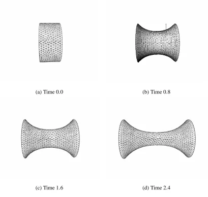
4.1 Liquid Bridge

The liquid-bridge problems considered here comprise an initially cylindrical fluid domain

pinned at static circular contact lines to two parallel vertical walls. The walls move with

an equal and opposite velocity, stretching the free surface, which must adjust such that the

fluid volume is conserved. The initial domain, a fluid cylinder of radius 1 and length 1,

is discretised with 3406 nodes and 2054 isoparametric quadratic tetrahedral elements. The

initial mesh is generated with a target uniform edge length of 01 and a constant time step of

0001 is used. In the absence of gravity (St0) the fluid domain evolves in an axisymmetric

manner. Figure 1 illustrates the free-surface shape at four instants during the simulation.

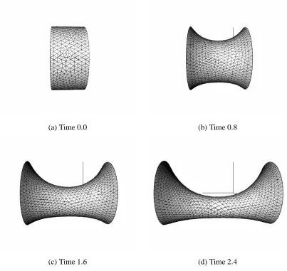
In the second example a gravitational force is introduced (St1) acting perpendicular to

the initial axis of symmetry of the fluid. The capillary number Ca1 in both examples.

Figure 2 illustrates the free-surface shape at the same four instants during this simulation.

Due to the motion of the solid boundaries, the edge length on the free surface neighbouring

the walls is increased relatively quickly, which necessitates regular discrete remeshing of the

domain. This is because the kinematic boundary condition (10) constrains the nodes on the

free surface to move in only the direction normal to it and hence the mesh becomes distorted

near the solid walls, which are moving almost tangentially to the free surface in the early

stages of the simulation. The examples shown have been remeshed twelve times during the

simulation. Since the volume remains theoretically constant during the simulation the number

there is a small volume change, due to both the discrete nature of the computational algorithm

employed and the occasional remeshing of the entire domain. In the two examples considered,

the volume change is approximately 05% of the initial volume over the entire simulation.

However, almost all of the observed error is introduced at the discrete remeshing stages, which

introduces a volume change which is an order of magnitude greater than that due to the explicit

update of the free surface.

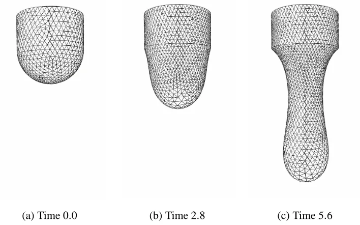
4.2 Droplet Formation

The droplet-formation problem comprises a vertically aligned cylindrical tube of radius 1 with

fluid fed into the top through a uniform parabolic velocity field. At the bottom the initially

hemispherical free surface of the fluid grows to accommodate the increase in fluid volume.

Hence, physically, the problem is a model of a slowly-forming drip on a leaking tap. The

contact line, where the fluid free-surface meets the opening of the tube, is fixed and treated as

static. For this example, the zero-gravity case is not particularly interesting since the droplet

will just develop, under the equilibriating action of surface tension, as an expanding sphere

attached to the cylindrical tube. Hence we only provide results where gravity is present,

act-ing in the axial direction of the tube. The initial mesh is generated with a target uniform edge

length of 01 and a constant time step of 0001 is used. Figure 3 illustrates the free surface

shape at three instants during a simulation in which the Stokes number St2 and Capillary

number Ca1. As the domain expands the mesh movement algorithm redistributes the

inter-nal nodes to allow for the boundary motion. Thus the mesh size necessarily grows, requiring

remeshing of the fluid domain, giving a corresponding increase in the discrete problem size

as time evolves. In the case shown in Figure 3(a) there are initially 2514 nodes and 1430

ele-ments while after six remeshing stages (Figure 3(c)) there are 4938 nodes and 2639 eleele-ments.

This has implications for the cost of the iterative solution at each time step. If an optimal

pre-conditioner were used the number of iterations would remain fixed but the cost per iteration

would grow. However, since our simpler preconditioner is not optimal the number of

itera-tions, as well as the cost per iteration, grows with the problem size. This issue of deteriorating

convergence rate still needs to be addressed in order to simulate the formation of the droplet

5

DISCUSSION AND FURTHER WORK

In this paper we have introduced an adaptive algorithm for the solution of three-dimensional

moving-boundary problems based primarily upon the use of mesh movement but also

exploit-ing discrete remeshexploit-ing when necessary. Previous work in this area has been typically based

upon linear tetrahedral or hexahedral finite element approximations, however here the

gov-erning equations are discretised with an a priori stable tetrahedral Taylor-Hood finite element

method. This method requires no additional artificial stabilisation and includes an

isopara-metric quadratic approximation of the problem geometry allowing a more accurate model of

the evolving free surface and of the surface tension forces acting on it. Application of this

algorithm to two fully three-dimensional problems has been described in order to demonstrate

the significant potential of the approach. At this stage, however, further development is still

required in order to ensure that this potentially powerful approach can be made sufficiently

robust to be applied to the widest possible range of free-surface flow problems.

At present the free surface is updated by allowing normal motion in order to satisfy the

kinematic boundary condition (10). It would be advantageous to allow free-surface nodes

to move in tangential directions as well since this is likely to reduce the frequency of the

discrete remeshing stages that is required. In the early stages of the liquid-bridge problem

considered in Section 4.1, the end planes are moving almost tangentially to the free surface

and so stretching occurs in the elements near to these planes: this could be avoided if suitable

tangential motion of the free-surface nodes was allowed.

Discrete remeshing is vital if long-time simulations of evolving fluid surfaces are to be

achieved. The simple rules described in Section 3.4 for driving the remeshing process can be

enhanced in a number of ways, to include for example other measures of surface mesh quality,

and further investigation is required to produce a precise strategy. In addition to the

computa-tional cost associated with the discrete remeshing stage, our current implementation (based up

on the use of the NETGEN software tool [28]) also causes a small, but not negligible, change

in the volume of the fluid. It is necessary therefore to investigate the most effective way of

eliminating this volume change from the remeshing procedure. Numerous approaches are

possible, however it is important to ensure that local accuracy in the geometry representation

is maintained as well as global volume conservation.

in-creases with the problem size. Optimal preconditioners for Stokes and Navier-Stokes

prob-lems have been presented by [11], which bound the number of iterations required

indepen-dently of the mesh size, based on an optimal inner solve of the discrete Laplace equation

using a multigrid method. For the unstructured tetrahedral grids employed here, this approach

is not directly applicable, since the required hierarchy of grids is not available. However,

re-cent work [22] has suggested the use of algebraic multigrid techniques for this component of

the method.

The examples provided in this paper show the performance of the algorithm on problems

for which the contact line is fixed. In addition to problems of this type, those in which the

contact line moves, containing a so-called dynamic contact line, are of significant practical

interest. Examples include the spreading of a droplet across a surface or the capillary rise of a

fluid in a narrow tube. This is an extension of the work we are currently undertaking, initially

through the approach presented in [1].

Acknowledgements

The authors wish to thank the EPSRC for funding this work through grant GR/R25453/01.

A

THE SURFACE DIVERGENCE THEOREM

In the notation of Subsection 3.1 the surface divergence theorem, [37], states that

Γf

∇sv dΓ

γv m dγ

Γf

2HvndΓ (21)

where H

1

2∇sn is the surface mean curvature. Hence, application of (21) with v

1

Caφieα

(where eα is the unit vector in coordinate directionα) gives:

Γf

∇s

1

Caφieα dΓ γ 1

Caφieα

m dγ

Γf

∇sn

1

Caφieα

n dΓ (22)

Hence Γf φi 1 Ca

∇snneαdΓ

Γf

1

Ca∇s

φieαdΓ

γ

1

Caφim

eαdγ (23)

Γf

1

Ca∇sφieαdΓ

γ

1

Caφimeαdγ (24)

References

[1] Baer, T.A., Cairncross, R.A., Schunk, P.R., Rao, R.R., and Sackinger, P.A. (2000). A

finite element method for free surface flows of incompressible fluids in three dimensions.

Part II. Dynamic wetting lines. Int. J. Num. Meth. Fluids. 33, 405-427.

[2] Bonet, J. and Peraire, J. (1991). An alternating digital tree (ADT) algorithm for 3d

geo-metric searching and intersection problems. Int. J. Num. Meth. Engg. 31, 1-17.

[3] Bunner, B. and Tryggvason, G. (1999). Direct numerical simulation of three-dimensional

bubbly flows. Phys. of Fluids (Letters). 11, 1967-1969.

[4] Cairncross, R.A., Schunk, P.R., Baer, T.A., Rao, R.R., and Sackinger, P.A. (2000). A

finite element method for free surface flows of incompressible fluids in three dimensions.

Part I. Boundary fitted mesh motion. Int. J. Num. Meth. Fluids. 33, 375-403.

[5] Cerne, G., Petelin, S. and Tiselj, I. (2002). Numerical errors of the volume-of-fluid

in-terface tracking algorithm. Int. J. Num. Meth. Fluids. 38, 329-350.

[6] Gaskell, P.H., Jimack, P.K., Sellier M. and Thompson, H.M. (2004). Efficient and

accu-rate time adaptive multigrid simulations of droplet spreading. Int. J. Num. Meth. Fluids.

(To appear).

[7] Gaskell, P.H., Jimack, P.K., Sellier M., Thompson, H.M. and Wilson, M.C.T. (2004).

Gravity-driven flow of continuous thin liquid films on non-porous substrates with

topog-raphy. J. Fluid Mech.. (To appear).

[8] Gaskell, P.H., Savage, M.D., Summers J.L. and Thompson, H.M. (1995). Modelling and

analysis of meniscus roll coating. J. Fluid Mech.. 298, 113-137.

[9] Gresho, P.M., and Sani, R.L. (2000). Incompressible Flow and the Finite Element

Method. Volume 2: Isothermal Laminar Flow. Wiley.

[10] Hirt, C.W. and Nichols, B.D. (1981). Volume of fluids methods for the dynamics of free

boundaries. J. Comput. Phys.. 39, 201-225.

[11] Kay, D., Loghin, D. and Wathen, A.J. (2001). A preconditioner for the steady-state

[12] Kuiken, H.K. (1990). Viscous sintering: the surface-tension-driven flow of a liquid form

under the influence of curvature gradients at its surface. J. Fluid Mech.. 214, 503-515.

[13] Lynch, D.R. and O’Neill, K. (1981). Continuously deforming finite elements for the

so-lution of parabolic problems, with and without phase change. Int. J. Num. Meth. Fluids.

17, 81-96.

[14] Marar, O.K. and Troians, S.M. (1999). The development of transient fingering patterns

during the spreading of surfactant coated films. Phys. of Fluids. 11, 3232-3246.

[15] Mashayek, F. and Ashgriz, N. (1995). A spine-flux method for simulating free surface

flows. J. Comput. Phys.. 122, 367-399.

[16] Miyata, H. (1986). Finite difference simulation of breaking waves. J. Comput. Phys.. 65,

179-214.

[17] Moriarty, J.A., Schwartz, L.W. and Tuck, E.O. (1991). Unsteady spreading of thin liquid

films with small surface tension. Phys. of Fluids. 3, 733-751.

[18] Muttin, F., Coupez, T., Bellet M. and Chenot, J.L. (1993). Lagrangian finite-element

analysis of time-dependent free-surface flow using an automatic remeshing technique –

application to metal casting. Int. J. Num. Meth. Engg. 36, 2001-2015.

[19] Osher, S. and Sethian, J.A. (1988). Fronts propagating with curvature-dependent speed:

algorithms based on Hamilton-Jacobi formulations. J. Comput. Phys.. 79, 1-49.

[20] Peterson, R.C., Jimack, P.K., and Kelmanson, M.A. (1999). The solution of

two-dimensional free-surface problems using automatic mesh generation. Int. J. Num. Meth.

Fluids. 31, 937-960.

[21] Peterson, R.C., Jimack, P.K., and Kelmanson, M.A. (2001). On the stability of viscous,

free-surface flow supported by a rotating cylinder. Proc. Roy. Soc. Lond. A457,

1427-1445.

[22] Powell, C.E. and Silvester, D.J. (2002). Black-box preconditioning for mixed

formula-tion of self-adjoint elliptic PDEs. Numerical Analysis Report No. 415. Dept. of

[23] Pozrikidis, C. and Thoroddsen, S.T. (1991). The deformation of a liquid film flowing

down an inclined plane wall over a small particle arrested on the wall. Phil. Trans. Roy.

Soc. A340, 1-45.

[24] Ramaswamy, B. and Kawahara, M. (1987). Lagrangian finite-element analysis applied

to viscous free-surface fluid flow. Int. J. Num. Meth. Fluids. 7, 953-984.

[25] Saito, H. and Scriven, L.E. (1981). Study of coating flow by the finite element method.

J. Comput. Phys. 42, 53-76.

[26] Scardovelli, R. and Zaleski, S. (1999). Direct numerical simulation of free-surface and

interfacial flow. Annual Rev. Fluid Mech. 31, 567-603.

[27] Schmidt, A. (1996). Computation of three dimensional dendrites with finite elements. J.

Comput. Phys. 125, 293-312.

[28] Sch¨oberl, J. (1997). NETGEN - An advancing front 2D/3D-mesh generator based on

abstract rules. Comput. Visual. Sci. 1, 41-52.

[29] Schwartz, L.W. and Eley, R.R. (1998). Simulation of droplet motion on low-energy and

heterogeneous surfaces. J. Colloid Inter. Sci. 202, 173-188.

[30] Sethian, J.A. (1996). Level Set Methods: Evolving Interfaces in Geometry, Fluid

Me-chanics, Computer Vision and Material Sciences. Cambridge University Press:

Cam-bridge, UK.

[31] Soulaimani, A. and Saad, Y. (1998). An arbitrary Lagrangian-Eulerian finite element

method for solving three-dimensional free surface flows. Comput. Meth. Appl. Mech.

Engrg. 162, 70-106.

[32] Stone, H.A. (1994). Dynamics of drop deformation and breakup in viscous fluids. Annual

Rev. Fluid Mech. 26, 65-102.

[33] Struik, D.J. (1961). Differential Geometry (second edition). Adison-Wesley.

[34] Tom´e, M.F., Filho, A.C., Cuminato, J.A., Mangiavacchi, N. and McKee, S. (2001).

GENSMAC3D: a numerical method for solving unsteady three-dimensional free surface

[35] van der Vorst, G.A.L. and Mattheij, R.M.M. and Kuiken, H.K. (1992). A boundary

ele-ment method for two-dimensional viscous sintering. J. of Comput. Phys.. 100, 50-63.

[36] Walkley, M.A., Gaskell, P.H., Jimack, P.K., Kelmanson, M.A., Summers, J.L., and

Wil-son, M.C.T. (2004). On the calculation of normals in free-surface flow problems. Comm.

Num. Meth. Engrg. (To appear).

[37] Weatherburn, C.E. (1939). Differential Geometry of Three Dimensions. Cambridge

Uni-versity Press.

[38] Zhou, H., and Derby, J.J. (2001). An assessment of a parallel, finite element method

for three-dimensional, moving-boundary flows driven by capillarity for simulation of

(a) Time 00 (b) Time 08

(c) Time 16 (d) Time 24

(a) Time 00 (b) Time 08

(c) Time 16 (d) Time 24

(a) Time 00 (b) Time 28 (c) Time 56