Comparative Analysis of Dynamic Electrochemical Test Methods of Supercapacitors

Int. J. Electrochem. Sci., 9 (2014) 7110 - 7130

International Journal of

ELECTROCHEMICAL

SCIENCE

www.electrochemsci.org

Comparative Analysis of Dynamic Electrochemical Test

Methods of Supercapacitors

Z. Stevic1,*, M. Rajcic-Vujasinovic1 and I. Radovanovic2

1

University of Belgrade, Technical faculty, Bor, Serbia

2

Innovation center of School of Electrical Engineering, University of Belgrade, Belgrade, Serbia

*

E-mail:[email protected] ; [email protected]

Received: 9 September 2013 / Accepted: 26 June 2014 / Published: 29 September 2014

Supercapacitor investigation due to the high capacitance, therefore long time constants, requires considerable modification and adaptation of classical electrochemical methods and instrumental techniques. This paper presents a mathematical analysis, which defines the parameters of the experimental methods, modified standard methods (galvanostatic, potentiostatic, ALSV), as well as new one - tilting current excitation. Firstly, the methods are tested on a specially constructed physical model - the electrical circuit with commercial super capacitor of 1.6 F, as well as the computer simulation. The measurements were performed on a specially developed measuring system based on PC and LabVIEW package. All the methods are applied in the development of a new type of supercapacitor based on natural copper minerals - chalcocite (Cu2S). Comparative methods analysis in

terms of efficiency and accuracy is given in the paper.

Keywords: Supercapacitors, Electrochemical methods, Mathematical Model, LabVIEW, Equivalent electrical circuit

1. INTRODUCTION

There are a number of standard methods for the examination of electrochemical systems that are used for supercapacitor testing [1-8]. In this paper, most important standard methods are presented along with their modification proposals, and also some more suitable methods for testing various supercapacitor parameters are presented.

and counter electrode is made of platinum or other conductive material which is insoluble in that particular electrolyte.

Depending on the wanted accuracy, possible duration of the test or equipment availability, different electrochemical system testing methods are applied. Comparative analysis of the most suitable dynamic methods for supercapacitor testing is presented in this paper.

2. PROCESS MODELING DUE TO DIFFERENT EXCITATIONS

Different signal excitations are defining particular testing methods for electrochemical systems. For this analysis, the following methods have been chosen: galvanostatic, potentiostatic, swiping voltage and current and cyclic voltammetry. For every particular method, mathematical model is derived and system response is defined for given excitation. Also, the algorithms for system parameters extraction are given, based on experimentally obtained response diagrams.

2.1. Galvanostatic Method

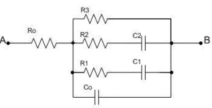
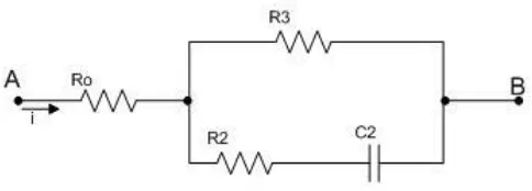
In galvanostatic electrochemical method, excitation of a system is pulse current of constant intensity (I) and the settable duration [1,10-12].

Response, the voltage between the working electrode (WE) and the reference electrode (RE) is being monitored on an electronic milivoltmer and plotter (EMVP) or, more recently through AD converters on the computer [13]. It is important that the input resistance EMVP has to be very high (order of 1012 Ω or more) because of the reference electrode tremendous internal resistance. In electrochemistry this specified voltage is often called overvoltage [1] (referring to the additional voltage between WE and RE given in regard to the voltage between these electrodes when there is no excitation current).

Figure 1. Equivalent circuit for the observed class of electrochemical systems

which response to the galvanostatic pulse is practically the same as for the observed electrochemical system (Fig. 1.) [10, 11, 14-24].

Resistance Ro physically corresponds to the resistance of the electrolyte and the electrode material together, and its value is in the order of ohms. Capacitance Co (order of magnitude μF) corresponds to the dual layer that is formed on the side of the electrolyte. Resistance R1 and R2 (the

order of magnitude of tens of ohms) are related to the slow processes of adsorption and diffusion, as well as the capacitor C1 (mF) and C2 (F). R3 is the resistance of self-discharge, so it is reciprocally

connected with electricity leakage. Its value is in the order of hundreds of ohms to several kilohms. Taking into account the magnitudes of capacitance C0, C1 and C2, the secondary region of

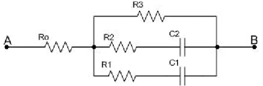
galvanostatic pulses, it is possible to simplified the equivalent circuit by omitting the capacitor C0,

which is not an essential when it comes to supercapacitors (Fig. 2.).

Figure 2. Simplified equivalent circuit

Complex images of overvoltage η, ie voltage UAB is:

) ( ) ( ) ( ) ( )

( Z S

S I S Z S I S U

S  _AB   _AB  _AB



























/ ) ( 2 2 1 1 3 2 1 2 1 2 1 3 2 1 2 1 2 3 2 3 2 1 3 1 2 1 3 2 1 2             C R C R R C C S C C R R R C C R R S S R C R R C R R S C C R R R S I S I R S O 

The resulting expression is quite complex, but it can be significantly simplified assuming that C2>>C1, which is physically realistic. By applying the Heaviside expansion formula overvoltage is

obtained in the time domain:





 ₁ 1 ₁  2

) ( 3 2 2 3 23    t t

O I e

R R R e I R R t

or in a slightly different form:









 ₁ 1 ₁  2

)

( ₂₃  _{3 23} 



t t

O R I e R R I e

R t whereby: 3 2 3 2 23 R R R R R 





 (time constant of the first phase)





 (time constant of the second phase)

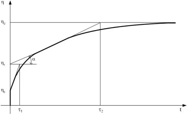
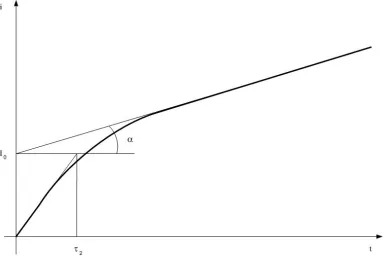
Typical appearance of galvanostatic curve with characteristic data from which it is possible to calculate all parameters of equivalent circuit is shown in Fig 3.

Figure 3. Typical galvanostatic curve of observed electrochemical systems

If a complete galvanostatic curve is recorded (during the pulse duration greater than 4 τ2 to

achieve a stationary level η2, which is quite a long time - the order of thousands of seconds), the

procedure for obtaining the parameters of the circuit would be as the following:

1. Evaluation of the value of Ro compared to the other resistance. If Ro cannot be ignored it is

necessary to make additional galvanostatic experiment with the same intensity of current, but with the time duration in order of μs. Then the intercept η on the axis is:

η00 = R0I (Co is short-circuit in such a short time)

which implies: I

R 00

0 



2. From the diagram (Fig 3.) it is obvious that: η2 =(R0 + R3) I

therefore: 2 ₀

3 R

I R  

therefore:









2 



 

 

I R R

I R R

R

4. From the diagram (Fig 3.):

η0 =(R0 + R123) I (R123 parallel connection R1 , R2 , R3)

therefore:









1 



 

 

I R R

R I R R

5. From the diagram (Fig 3.) time constant τ1 is:

τ1 = (R1 + R23) C1

therefore, the capacitance can be calculated:

23 1

1 1

R R C

  

6. From the diagram (Fig 3.) time constant  2 is:

 2 = (R2 + R3) C2

therefore, C2 can be calculated:

3 2

2 2

R R C

  

It should be noted that the C2, as the most important parameter of the circuit when it comes to

supercapacitors, can be determined from a short pulse of galvanostatic, from the slope of the linear part of the galvanostatic curve. The only problem is that firstly it is necessary to determine the resistance R3

(potentiostatic method or some other method). For determined R3 and calculated R2 following the

instuctions given in the point 3. of this method, C2 can be determined from:





2 3

C I R R

R tg

 

 





I R

C ₂

3 2

2 3 2

 

Where, tg (Fig 3) is the slope of the linear part of the galvanostatic curve, ie. the numerical value of derivative

dt d

in that area, expressed in V / s.

2.2. Potentiostatic Method

In this method, the excitation is a constant impulse overvoltage E, and the response is monitored as current change in time, therefore, this method is often referred to as chronoamperometry [1].

Voltage and its complex image is:

) ( )

(t Eh t

 ,

S E S) (

 ,





















1 ) ( 1 ) ( ) ( 2 2 1 1 3 2 1 2 1 2 1 3 2 1 2 1 2 3 2 3 2 1 3 1 2 1 3 2 1 2 0               C R C R R C C S C C R R R C C R R S R C R R C R R S C C R R R S R S E S Z S S i 

Taking into account the actual fact that C2>>C1, by applying the Heaviside expansion formula,

the current in the time domain is:









)

(t I I e I I e I

i t t        where: 123 0 0 R R E I 

 - initial charging current

23 0 1 R R E I 

 - final first-phase charging current

3 0 2 R R E I 

 - final charging current

1 1 0

1 (R R )C

 - time constant of the first phase

2 2 0

2 (R R )C

 - time constant of the second phase

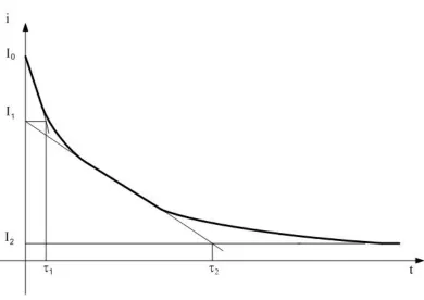
In Figure 4 shows the current diagram according to the given expression.

Figure 4. Potentiostatic excitation, current diagram

0 2

3 R

I E

R  

0 1

23 R

I E

R  

23 3

3 23 2

R R

R R R





0 0

123 R

I E

R  

123 23

23 123 1

R R

R R R

 

1 0

1 1

R R C

  

2 0

2 2

R R C

  

This method has two major advantages over the other ones. Resistance R3 can be the most

reliably determined from the clearly discernible horizontal part of the curve, and also the time of the experiment is the shortest (lowest time constant of the second phase of charging).

2.3. Linear Sweep Voltage Excitation

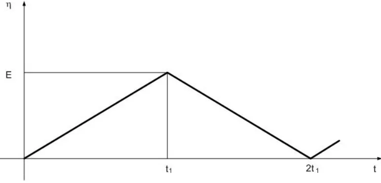
System excitation is linear sweep voltage function as shown in Fig 5. The current in time as a response is monitored.

Figure 5. Linear sweep voltage function

Figure 6. Equivalent circuit for second charging phase

The equation for the overvoltage in the time and frequency domain is:

T S E S t h t T E t 2 ) ( ) ( ) (      

Impedance of the circuits is:









Complex image of current is:

) ( ) ( ) (( ( 1 ) ( ) ( ) ( 3 2 0 3 2 2 2 3 2 2 S Q S P T E R R R R R SC S R R SC T E Z S S I       

Back in the time domain was carried out by the following procedure: Q = 0  S1 = 0; S2 = 0;

) )

(( 2 3 0 2 3)

2 3 0 3 R R R R R C R R S     

Usually R0 << R2 << R3, therefore:

2 2 0 3 ) ( 1 C R R Q    3 2 0 3 2 2 2 3 0 0 3 2 3 2

2(( ) ) (( )

(

2S SC R R R R R R R S C R R R R R

Q       

2 3 3) ( R R S

P 

3 0 1 1 R R k   3 3 2 2 2 3 0 3 3 2 2 ) ( ) ( R R R C R R R R R

k  

           _               

 1 2 3  2

3 3 2 2 3 3 2 2 3 0 3 3 2 1 1 ) ( ) ( ) (  t t S t S t S e R R R C R R R C t R R T E e S Q S P e k e t k T E t i 2 2 0

2 (R R )C 

Figure 7. Current response diagram

Reading the values from the diagram, tgα, I0 and τ2 (with the previously determined or estimated parameter R0), parameter R3 can be calculated:

0

3 R

tg T

E

R 

 

 ; t

I tg

  

 (linear part of the curve) From the system of equations:

2 3

3 2 0

) (

C R

R R

I  

2 2 0

2 (R R )C 

R2 and C2 can be calculated.

In this way, the most important parameters of a supercapacitor have been determined, while at the same experiment is short term, and the destruction of the electrode is low.

2.4. Cyclic Voltammetry

Figure 8. Excitation signal for cyclic voltammetry

As the response, input current in the time domain is monitored. Common name in electrochemistry is cyclic voltammetry, although the current is being measured, because the voltage at which current peak occurs is essential. In the case of supercapacitor, peaks are not expressed, because of the slow changes.

Excitation voltage can be expressed analytically as: 

) (t

 t

t E_m

1

for the arising area (charging phase) 

) (t

 t

t E

E_m m

1

2  for the falling area (discharge phase)

With the realistic assumption that R0 << R3 and adding the condition t1 > 4R2C2 - time constant, by using the procedure similar to the linear sweep voltage function it leads to a simplified expressions for the current in the time domain in the quasi-stationary mode:

3 2

1 2

2 1 )

( 2

R E e

C t E t

i m

t m

     

  



 

charge phase

3 2

1 2

1 2

)

( 2

R E e

C t E t

i m

t m

     

  



 

discharge phase

The time is measured from the beginning of each stage. Obviously this is a complex form of current in time with exponential change of the AC component, and the DC component whose level is

3

2R E

I m

DC  , therefore:

2 1 3 max

2 t C

E R E

I  m  m ; ₂

1 3 min

2 t C

E R E

2 1 min max

2 t C

E I

I _m

 

Time diagram of the current is presented in the Fig. 9.

Figure 9. Responsive system current

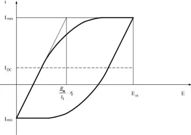
Usually with this method, current is shown as the function of the excitation voltage, so the graph is obtained as shown in Fig 10.

Area of the shown loop (the electric power) is:





  

  

  

 1  2

0 1

2 1 0

2 1 2

2

t

m t m

Em

p dt

t E e C

t E id

S  

) 2 (

2 _{2 1 2}

2 1

2





 C t

t E

S m

p

Based on these expressions, the procedure for the determination of the two most important supercapacitor parameters is:

1. From the recorded diagram as shown in Fig. 9, getting the values Imax and Imin so that the capacitance C2:

1 min max 2

2E t

I I C

m

 

2. From the same diagram, getting the time constant τ2, therefore the resistance R2 can be calculated:

2 2 2

C R  

It should be noted that C2 can be determined from the expression for the loop surface that is

more complex, but approximately applicable even if the experiment is not lead to the attainment of Imax, therefore it has shorter duration.

2.5. Linear Sweep Current Excitation

Figure 11. Diagram of linearly sweep current excitation

In this case, as the excitation it is applied linear current change over time (Fig 11.), and overvoltage η in charge was observed as a response. Depth analysis showed that this method clearly separates the first from the second charging phase (ie C1 and C2), so it is more suitable for reliable

determination of the most important supercapacitor parameters, primarily C2. Therefore, in this section

Therefore, the analysis of the second charging phase, more precisely the segment from which the important supercapacitor parameters can be determined, is presented in this paper.

For the observed charging phase, system equivalent circuit is reduced to the one presented in Fig 11.

The expression for the current in the time and frequency domain is:

) (t h t T I

i 

T S

I S I( ) ₂

Circuit impedance is the same as in linear sweep voltage excitation, so the complex image of overvoltage:













S _AB 

          

Since the polynomial Q (S) has a double root, the inverse Laplace transformation procedure is as follows.

; 0 0 ₁

 S

Q S₂ 0;





2 3 1 R R C S   













2 3

2

2 1

2S SC R R S C R R

Q    

3 2 2 3 3) ( R R R S P  





2 3 1 ) ( R R C S Q    3 0 1 1 2 1 ) ( ) ( R R S Q S P S

K   

2 2 3 2 2 2 2 ) ( ) ( C R S Q S P s ds d

K _

              

 St St St

e S Q S P e k te k T I

t 1 2 3

) ( ) ( ) ( 3 3 2 1 





  2

2 2 3 2 2 3 3 0 ) (   t e C R C R t R R T I t

where τ2 = (R2 + R3)C2 – time constant of the second phase of charging.

The expression for the overvoltage in the time domain is shown graphically in Fig 12. The equation of the asymptote for the presented graph is obtained from:









2 3 3 0 )

( R R t R C

T I

t t   



Therefore, the intercept on the ordinate and the slope of the line are:

2 2 3

0 R C

T I   





T I

Figure 12. Diagram of the overvoltage

By getting η0 and k from the diagram and including the values in the last two equations, the R3

and C2 can be determined, assuming that R0 is determined by another method, or that it is negligible

compared to R3.

3. RESULTS AND DISCUSSION

Electrochemical experiments have been performed in a standard three-electrode cell with saturated calomel reference electrode. Platinum electrode was used as a counter electrode [1,27-31]. Several working electrodes of different materials have been examined. This paper presents the results of the electrodes of chalcocite (Cu2S, natural copper mineral).

Aqueous solutions of sulfuric acid, copper sulfate, sodium carbonate and sodium chloride p.a. purity have been used as electrolyte.

For each series of experiments, the working electrodes were honed, polished, washed and dried and then immersed in an electrolyte that was also fresh for the new series. Between the two experiments of the same series, polishing with rinse was performed. Grinding has been done with the finest sandpaper, polishing with alumina and rinsing with distilled water and alcohol.

All of the experiments were conducted at room temperature.

Physical model have been made according to the scheme in Figure 1, and it have been used for additional verification of the method. The values of the parameters: R0 = 3 Ω; R1 = 39 Ω; R2 = 90 Ω;

3.1. Modified Galvanostatic Method

Galvanostatic experiments were performed according to previously described modified method for all of the working electrodes in various electrolytes. Starting from the adopted model, the parameters of equivalent electrical circuit for each system were determined and based on that further experiments were performed.

Figure 13. Physical model response on the galvanostatic excitation

Figure 14. Galvanostatic curve for calcocite in a solution 1M H2SO4+0,1M CuSO4 at excitation of

Firstly, method and instrumental technique in the previously described physical model were checked once again. The intensity of the current pulse was 3 mA, and duration 40 s. The response of the circuit is shown in Fig. 13.

By getting characteristic values from the diagram and inserting those values into mathematical model, described previously in the analytical section, it is possible to define the parameters of the circuit:

R1 = 38,6 Ω; R2 = 91,5 Ω; C1 = 29,2 mF; C2 = 1,56 F

which is in full compliance with the actual values. To determine the required R3, much longer

experiment is needed, therefore this parameter is omitted.

Galvanostatic curve for chalcocite electrode (which was considered the most appropriate for) in a solution of sulfuric acid with the addition of copper sulfate at 0.1 mA excitation for a period of 20000 s is shown in Fig. 14. According to the diagram equivalent circuit parameters were calculated:

R1 = 17,3 Ω; R2 = 31,2 Ω; R3 = 210 Ω; C1 = 0,23 F; C2 = 33,1 F

The obtained values will be compared later with results obtained by other methods.

3.2. Potentiostatic Method

Figure 15. Potentiostatic curve for physical model at excitation of η = 100 mV

The method was firstly tested on a physical model with parameters: R0 = 3 Ω; R1 = 39 Ω; R2 =

90 Ω; R3 = 150 Ω; C0 = 0,12 μF; C1 = 30 mF; C2 = 1,6 F. Excitation of η = 100 mV with duration of

900s. Potentiostatic curve is presented in Fig.15.

By getting the characteristic parameters of the diagram (as described in the analytical section), the most important parameters of the circuit were defined:

R2 = 91,1 Ω; R3 = 148,8 Ω; C2 = 1,63 F ,

which is in a full compliance with the actual parameters.

order to select the optimal electrolyte in terms of obtaining the highest capacitance with minimal current leakage, therefore, the maximum value of R3.

Figure 16 shows potentiostatic curve (excitation at η = 20 mV) for chalcocite electrode in 1 M sulfuric acid together with 0.1 M copper sulfate.

Figure 16. Potentiostatic curve for chalcocite electrode in solution of 1M H2SO4+0,1M CuSO4 at

excitation of 20 mV

For such a optimized system, circuit parameters were obtained: R1 = 17,1 Ω; R2 = 30,8 Ω; R3 =

206 Ω; C1 = 0,22 F; C2 = 31,8 F.

3.3. Cyclic Voltammetry

The classical method has been used with a very low speed voltage rise due to the high time constants of the investigated electrochemical systems.

The first measurements were conducted on a physical model with R0=3 Ω; R1=39 Ω; R2=90 Ω;

R3=1 kΩ; C0=0,12 μF; C1=30 mF; C2=1,6 F at a voltage increase speed of dE/dt = 1 mV/s. Fig. 17

shows diagrams for dE/dt = 1 mV/s. For the diagram obtained main parameters (R2 = 92 Ω , C2 = 1,63

F) are in full compliance with actual data. Results show that it should apply as slow change of voltage as possible in order to obtain a wider loop, therefore, to reduce measurement errors.

Series of experiments with a variety of electrochemical systems and different voltage increase speeds were conducted in order to find optimal working conditions.

Figure 18. Voltammogram for H2 in a solution of 1M H2SO4+0,1M CuSO4 at dE/dt = 10 μV/s

Fig. 18 shows the voltammogram for the selected electrode (chalcocite) and the chosen electrolyte (1M H2SO4+0,1M CuSO4) at voltage increase speed of 10 μV/s.

Surface of the loop was measured and from it the capacitance C2 was determined: C2 = 32,2 F.

Pulling the tangent to the initial part of the curve, time constant τ2 = 1034 s was determined, therefore

R2 =

2 2

C 

= 32,1 Ω.

3.4. Linear Sweep Current Excitation

Due to the longer duration of the experiment, few typical systems were tested by this method. Fig. 19 shows response of an adopted electrochemical system (chalcocite in 1M H2SO4 + 0,1M CuSO4)

at excitation di/dt = 1,5 nA/s.

Based on the experimental curve, the parameters of the circuit have been calculated: R2 = 30,9 Ω; R3 = 201 Ω; C2 = 33,4 F

Figure 19. Response of the adopted system at tilting current excitation

3.5 Comparative Methods Review

In this section, a short review of the advantages and disadvantages of the methods will be presented, as well as tabular overview of the results.

In the case that the expensive equipment is not available or it is necessary to quickly determine the certain individual parameters, it is possible to use one of the fastest methods. The experiments show that the potentiostatic method provides satisfactory results with a shorter duration of the experiment, and even quicker, although rougher parameter determination, galvanostatic method can be applied. For a reliable determination of the capacitance C2, cyclic voltammetry can be applied, but

with a long time experiment.

Table 1. below, shows the overview of the equivalent circuit parameters obtained by various methods for adopted electrochemical system.

Table 1. Overview of the measured parameters of the adopted electrochemical system

Method R1 [Ω] R2 [Ω] R3 [Ω] C1 [F] C2 [F]

Galvanostatic method

17,3 31,2 210 0,23 33,1

Potentiostatic method

17,1 30,8 206 0,22 31,8

Cyclic

Voltametry - 32,1 - - 32,2

Linear sweep current excitation

Since these are non-linear elements, and the methods are graphical, it can be concluded that the matching between the results is satisfactory. In addition to results matching of the methods described herein, well results matching has been found with the results obtained by other methods [32-34]. More accessible equipment has been used in here and developed mathematical models make it easier to conduct experiments.

4. CONCLUSION

Sulphide materials are poorly investigated from the standpoint of the electrode material for supercapacitors, therefore the presented researches are new to the area. The behavior of natural copper sulphide minerals, especially chalcocite (Cu2S) in a solution of sulfuric acid with and without addition

of CuSO4 has been examined. Especially well behavior chalcocite has shown in solution 1M H2SO4 +

0,1M CuSO4. The results suggest the possible application of the shown system (memory and other

electronic circuits with low power consumption), and also pave the directions of the further research in order to get even better parameters.

In order to do better investigation of the observed systems, the mathematical model is set, equivalent circuit was accepted and the comparative analysis was done for the standard electrochemical test methods (cyclic voltammetry and potentiostatic method), galvanostatic method is modified and new method is defined for this class of problems (linear sweep current excitation). Based on mathematical analysis all the parameters for experimental research are determined.

Series of the experiments has been conducted, both in the physical model and the real electrochemical systems. Based on obtained results, the model and test methods are verified, and also the electrochemical system is optimized. Also, the methods are compared in terms of efficiency and accuracy.

ACKNOWLEDGMENTS

The authors gratefully acknowledge financial support from the Ministry of Education and Science, Government of the Republic of Serbia through the Projects No. 172 060: “New approach to designing materials for energy conversion and storage” and Project No. 32043: “Development and modeling of energy efficient, adaptive, multi-processor and multi sensor low power electronic systems“.

References

1. B.E.Conway, Electrochemical supercapacitors, Kluwer Academic/Plenum Publishers, New York, (1999).

2. I.L. Skryabin, G. Evans, D. Frost, G. Vogelman and J.M. Bell, Electrochimica Acta, 44 (1999) 3203-3209.

3. P.C.Butler, J.F. Cole, P.A. Taylor, Journal of Power Sources, 78 1-2 (1999) 176-181.

4. A.D. Pasquier, I. Plitz, J. Gural, S.Menocal and G. Amatucci, Journal of Power Sources, 113 1 (2003) 62-71.

5. Конденсаторы. Методы измерения электрических параметров. Общие положения. ГОСТ 21315.0-75, Издательство стандартов, 1976.

7. Y. Guo, J. Qi, Y. Jiang, S. Yang, Z. Wang and H. Xu, Materials Chemistry and Physics, 80, 3 (2003) 704-709.

8. G. P. Dai, M. Liu, D.M. Chen, P. X. Hou, Y. Tong and H. M. Cheng, Electrochemical and Solid-State Letters, 5, 4 (2002) E13-E15.

9. Z. Stevic, Ph.D thesis, ETF Belgrade, 2004.

10.C. Arbizzani, M. Mastragostino and L. Meneghello, Electrochimica Acta, 41, 1 (1996) 21-26. 11.M. Rajčić-Vujasinović, Z. Stanković and Z. Stević, Elektrokhimiya, 35, 3 (1999) 347- 354. 12.C. Arbizzani, M. Mastragostino and F. Soavi, Journal of Power Sources, 100 (2001) 164-170. 13.Z. Stević, Z. Andjelković and D. Antić, Sensors 8, (2008) 1819-1831.

14.J.P. Zheng, J. Huang and T.R. Jow, Journal of the Electrochemical Society, 144, 6 (1997) 2026-2031.

15.J. Jamnik, J. Maier and S. Pejovnik, Electrochimica Acta, 44 (1999) 4139-4145.

16.W.C. West, K. Sieradzki, B. Kardynal and M.N. Kozicki, Journal of the Electrochemical Society, 145, 9 (1998) 2971-2974.

17.E. Barsoukov, J. H. Kim, K.S. Hwang, D. H. Kim, C.O. Yoon and H.Lee, Synthetic metals, 117, 1-3 (2001) 53-59.

18.P.J. Mahon, G. L. Paul, S. M. Keshishian and A. M. Vassallo, Journal of Power Sources, 91, (2000) 68-76.

19.Q. Yin, G.H. Kelsall, D.J. Vaughan and N.P. Brandon, Journal of the Electrochemical Society, 148, 3 (2001) A200-A208.

20.B. Pettinger and K. Doblhofer, Can. J. Chem. 75, 11 (1997) 1710-1720.

21.Ch. Lin, B. N. Popov and H.J. Ploehn, Journal of the Electrochemical Society, 149, 2 (2002) A167-A175.

22.H. Kim and B.N. Popov, Journal of the electrochemical society, 150, 9 (2003) A1153-A1160. 23.Hongqing Cao and Jingxian Yu, Evolutionary Computation, CEC '03. The 2003 Congress on,

(2003).

24.R. Martin, J. J. Quintana, A. Ramos and I. de la Nuez, Electrotechnical Conference, MELECON 2008, The 14th IEEE Mediterranean, (2008).

25.W.G. Pell and B.E. Conway, Journal of Electroanalytical Chemistry 500, 1-2 (2001) 121-133.

26.M. Rajčić-Vujasinović, V. Trujić, Z. Stević and S. Đorđević, 3rd International Conference of the Chemical Societies of the South-Eastern European Countries on Chemistry in the New Millennium – an Endless Frontier, Book of Abstarcts, Volume I (2002) 337.

27.M. Antonijevic and S. M. Milic, Materials chemistry and physics, vol. 118 No. 2-3 (2009) 385-391.

28.R. Markovic, J. Stevanovic, Lj. Avramovic, D. Nedeljkovic,B. Jugovic, Z. Branimir, J. Stajic-Trosic and M. Gvozdenovic, Metallurgical and materials transactions b-process metallurgy and materials processing science, vol. 43 No. 6 (2012) 1388-1392.

29.V.V. Panić, R.M. Stevanović, V.M. Jovanović and A.B. Dekanski, Journal of Power Sources, 195(13) (2010) 3969-3976.

30.V. Grekulovic, M. Rajcic-Vujasinovic, B. Pesic and Z. Stevic, International journal of electrochemical science, vol. 7 No. 6 (2012) 5231-5245.

31.H. Karami and A. Kaboli, International Journal of Electrochemical Science, 5(5) (2010) 706-719. 32.L. Borcea, Electrical impedance tomography, Inverse Problems, 18 (2002) R99-R136.

33.L. Kavan, P. Rapta and L. Dunsch, Chemical Physics Letters, 328 4-6 (2000) 363-368. 34.M. Itagaki, T. Ono and K. Watanabe, Electrochimica Acta, 44 (1999) 4365-4371.