R E S E A R C H
Open Access
Sparse reconstruction for direction-of-arrival
estimation using multi-frequency co-prime arrays
Elie BouDaher, Fauzia Ahmad
*and Moeness G Amin
Abstract
In this paper, multi-frequency co-prime arrays are employed to perform direction-of-arrival (DOA) estimation with enhanced degrees of freedom (DOFs). Operation at multiple frequencies creates additional virtual elements in the difference co-array of the co-prime array corresponding to the reference frequency. Sparse reconstruction is then used to fully exploit the enhanced DOFs offered by the multi-frequency co-array, thereby increasing the number of resolvable sources. For the case where the sources have proportional spectra, the received signal vectors at the different frequencies are combined to form an equivalent single measurement vector model corresponding to the multi-frequency co-array. When the sources have nonproportional spectra, a group sparsity-based reconstruction approach is used to determine the direction of signal arrivals. Performance evaluation of the proposed multi-frequency approach is performed using numerical simulations for both cases of proportional and nonproportional source spectra.
Keywords:Sparse reconstruction; Co-prime arrays; DOA estimation; Group sparsity
1 Introduction
Direction-of-arrival (DOA) estimation has been an area of continued research interest due to its wide range of applications in radar, sonar, and wireless communica-tions [1-3]. A main parameter in DOA estimation is the maximum number of sources that can be resolved. Traditional high-resolution DOA techniques, such as MUSIC [4] and ESPRIT [5], can only estimate up to (N−1) sources when applied to an Nelement uniform linear array (ULA). Numerous nonuniform array geom-etries and signal processing techniques have been intro-duced to increase the number of resolvable sources beyond that offered by a ULA for a given number of physical sensors [6-13].
Minimum redundancy arrays (MRAs) and minimum hole arrays (MHAs) are two common classes of nonuni-form linear arrays [6-9]. Both MRAs and MHAs provide the ability to resolve more sources than the number of physical sensors by reducing the number of redundant virtual elements in the difference co-array. The ence co-array is defined as the set of all pairwise differ-ences of array element locations, and thus, it specifies the set of ‘lags’at which the spatial correlation function
may be estimated [10,11]. For a given number of physical sensors, MRAs are arrays with the lowest possible redun-dancy and without any missing lags or‘holes’in the cor-responding co-array, whereas MHAs (also known as Golomb arrays) have a minimum number of holes and zero redundancy. More recently, nested co-prime array configurations have been proposed [12,13]. Nested struc-ture is obtained by systematically nesting two uniform linear subarrays, with one subarray assuming a unit inter-element spacing, and can provide O(N2) degrees of freedom (DOFs)_ using only N physical sensors. A nested array generates a co-array with no holes. The co-prime array consists of two uniform linear subarrays having M and N sensors with specific inter-element spacings, where M and N are co-prime, and offers O
(MN) degrees of freedom. The co-prime array produces a co-array that has both redundancy and holes.
High-resolution DOA estimation with nonuniform arrays can be accomplished based on two main approaches, namely, covariance matrix augmentation [14] and spatial smoothing method for covariance matrix construction [12,13,15]. In the former approach, the constructed aug-mented covariance matrix is not guaranteed to be posi-tive semi-definite and requires posiposi-tive definite Toeplitz completion [16,17]. The latter approach vectorizes the covariance matrix of the nonuniform array to emulate
* Correspondence:[email protected]
Center for Advanced Communications, Villanova University, Villanova, PA 19085, USA
observations at a virtual array whose sensor positions are given by the difference co-array. Since the source signals are replaced by their powers in this case, render-ing the source environment coherent, spatial smoothrender-ing is utilized to decorrelate the sources and to restore the rank of the corresponding covariance matrix. However, the spatial smoothing-based method can only be applied to that part of the difference co-array that has a contigu-ous number of elements without any holes, implying that this technique cannot fully utilize the DOFs offered by co-prime arrays.
In [18], multiple frequencies were employed to exploit all of the DOFs of co-prime arrays, thus, increasing the number of resolvable sources. Measurements made at carefully chosen additional frequencies were used to fill in the missing elements in the difference co-array [19]. In doing so, the filled part of the difference co-array is extended, which, in turn, increases the maximum number of sources resolved by high-resolution DOA estimation techniques. However, the increase in DOFs comes with a restriction on the sources’spectra. More specifically, the sources are required to have proportional spectra at the considered frequencies [18,20]. Although this method pro-vides the ability to utilize all of the DOFs of the co-prime array, only a small portion of the additional measurements at frequencies other than the reference frequency are used; the rest are discarded.
In this paper, sparse reconstruction is considered to make use of the full measurement set corresponding to the multi-frequency operation for DOA estimation with co-prime arrays. This enhances the DOFs beyond those offered by a single-frequency operation due to the add-itional virtual elements generated in the co-array under multi-frequency operation. For sources with proportional spectra, the observations at the different frequencies are cast as a single measurement vector model, which corre-sponds to a virtual array whose element positions are given by the union set of the difference co-arrays corre-sponding to the multiple operational frequencies. Sparse reconstruction can then be applied for estimating the directions of signal arrivals. For the case where the sources have nonproportional spectra, the source signal vectors corresponding to the different frequencies have a common support, as the sources maintain their DOA even if their power varies with frequency. The common structure property of the sparse source vectors suggests the applica-tion of a group sparse reconstrucapplica-tion. It is noted that sparse recovery was previously applied for DOA estima-tion with co-prime arrays in [21,22]; however, it was lim-ited to a single-frequency operation and did not consider enhancement of the DOFs of co-prime arrays through multi-frequency operation.
Performance evaluation of the proposed sparsity-based methods is conducted using numerical simulations. We
consider three different cases for DOA estimation using sparse reconstruction at multiple frequencies. In the first case, all sources are assumed to have the same bandwidth and all sensors operate at the same multiple frequencies. The second and third cases violate the above assumption with a subset of sensors only operat-ing at multiple frequencies and the sources havoperat-ing non-identical bandwidth but overlapping spectra.
The remainder of the paper is organized as follows. In Section 2, the multi-frequency signal model for co-prime arrays is presented. In Section 3, the sparse reconstruction-based DOA estimation for multi-frequency co-prime arrays under proportional spectra is discussed. The case of sources with nonproportional spectra is consid-ered in Section 4, and the group sparsity-based reconstruc-tion is presented. The performance of the proposed methods is evaluated in Section 5 through numerical simu-lations, and Section 6 concludes the paper.
Notation
Vectors and matrices are denoted by lowercase and uppercase bold characters, respectively. Superscript (.)T denotes the transpose of a matrix or a vector, whereas their conjugate transpose is denoted by superscript (.)H. The Kronecker product and the Khatri-Rao product [1] are denoted by the symbols⊗and ⊙, respectively. E{.} denotes the statistical expectation operator, vec(.) de-notes the vectorized form of a matrix which is obtained by stacking the columns of the matrix to form a long vector, and bdiag{∙} denotes block diagonal matrix.
2 Multi-frequency signal model
In its basic configuration, a co-prime array consists of two uniformly spaced linear subarrays. The first subarray has
Melements withNd0inter-element spacing, and the
sec-ond one hasNelements withMd0spacing, whereM and
Nare co-prime numbers, andd0=λ0/2 is the unit spacing
withλ0being the wavelength at a reference frequencyω0
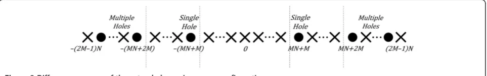
[13]. In this work, we deal with an extended co-prime array configuration, proposed in [15], which has twice the number of elements in one of the subarrays. More specif-ically, we assumeMto be less thanNwith the first subar-ray having 2M elements, as shown in Figure 1. The elements of the two subarrays are arranged along a single line with the zeroth elements coinciding, resulting in a co-prime array with a total of (2M+N−1) nonuniformly spaced physical elements. The difference co-array of the extended co-prime array can be expressed as:
S0¼ f ðMnd0−Nmd0Þg; ð1Þ
where 0≤n≤N −1, and 0≤m ≤2M −1. The co-array
elements between−(MN+M−1)d0and (MN+M−1)d0,
as depicted in Figure2.
Assume that Dsources are impinging on the (2M+
N−1)−element co-prime array from directions [θ1,θ2,
…,θD], whereθ is the angle relative to broadside. The
(2M+N−1) × 1 received data vector is expressed as:
xð Þ ¼ω0 Að Þω0 sð Þ þω0 nð Þω0 ; ð2Þ
wheres(ω0) = [s1(ω0)s2(ω0)…sD(ω0)]Tis the source
sig-nal vector at ω0, andn(ω0) is the (2M+N−1) × 1 noise
vector at ω0. The (2M+N −1) ×D matrix A(ω0) is the
array manifold at ω0, whose columns are the steering
vectors corresponding to the sources directions. That is,
A= [a(θ1) a(θ2)… a(θD)] with the steering vector a(θd)
corresponding to the directionθdgiven by:
að Þ ¼θd ejk0x1sinð Þθd ;…; ejk0x2MþN−1sinð Þθd
h iT
: ð3Þ
Here,k0= 2π/λ0is the wavenumber at the reference
fre-quencyω0, andxi,i=0, 1,…, 2M+N−1, is the location of
the ith array element. Assuming that the sources are uncorrelated and the noise is spatially and temporally white with varianceσ2
nand uncorrelated from the sources,
the autocorrelation matrix of the received data is given by:
Rxxð Þ ¼ω0 E xð Þω0 xð Þω0 H
n o
¼Að Þω0 Rssð Þω0 AHð Þ þω0 σ2nI; ð4Þ
whereRss(ω0) is the source correlation matrix which is
di-agonal with the source powers atω0, σ21ð Þω0 ;σ22ð Þω0 ;…;
σ2
Dð Þω0 ;populating its main diagonal, andIis a (2M+
N −1) × (2M+N −1) identity matrix. In practice, the
autocorrelation matrix is estimated as a sample average of the received signal snapshots.
Following the formulation in [13], the autocorrelation matrix is vectorized as:
zð Þ ¼ω0 vecðRxxð Þω0 Þ ¼A~ð Þω0 pð Þ þω0 σ2nð Þω0 ~i; ð5Þ
where Ã(ω0) =A*(ω0)⊙A(ω0) = [a*(θ1)⊗a(θ1) … a*
(θD)⊗a(θD)], p(ω0) is the sources powers vector at
ω0, pð Þ ¼ω0 σ21ð Þσω0 22ð Þ…ω0 σ2Dð Þω0
T
, and ĩ is the
vectorized form ofI. The vectorz(ω0) behaves as the
re-ceived signal vector at a longer virtual array with sensor
positions given by the difference co-array at ω0 of the
physical array. In this model, the sources are replaced by their respective powers and, as such, act as mutually co-herent sources, and the noise is deterministic. Traditional subspace-based high-resolution methods, such as MUSIC, can no longer be applied directly to perform DOA estima-tion. Spatial smoothing can be used to restore the rank of
the correlation matrix of z(ω0) [23]. However, it can only
be applied to the filled part of the difference co-array and the usable DOFs are reduced to approximately one-half of the total number of contiguous co-array elements. Sparsity-based DOA estimation can help extend the usable DOFs to
the number of positive lags in the co-array [24].
Consider operating the physical co-prime array at Q
different frequencies with the qth frequency given by
ωq=αqω0, where αq is a constant. Note that it is not
required for the reference frequencyω0to be one of the
Qoperational frequencies. If it is included in the oper-ational frequency set, the corresponding αq assumes a
unit value. The received signal at each considered fre-quency can be extracted by decomposing the array out-put vector into multiple nonoverlapping narrowband components by using the discrete Fourier transform (DFT) [25,26]. The observation time is assumed to be sufficiently long to resolve the different frequencies.
Figure 1Extended co-prime array configuration.
The received signal vector corresponding to the qth operational frequency can be expressed as:
x ωq ¼A ωq s ωq þn ωq : ð6Þ
array manifold of a scaled version of the physical
co-prime array, with the position of theith sensor in this
scaled array given by αqxi. This, in turn, results in the
difference co-array atωq to be a scaled version of the
difference co-array of Figure 2 (at the reference
fre-quencyω0), withαqbeing the scaling factor [19]. If ωq
is higher than the reference frequency,ω0, the co-array
atωqis an expanded version of the one at the reference
frequency. On the other hand, for ωq lower than ω0,
the equivalent co-array atωqis a contracted version of
that in Figure2. For illustration, consider an extended
co-prime array with M = 3 and N = 7 and the sensor
positions given by [0d0 3d0 6d0 7d0 9d0 12d0 14d0
15d0 18d0 21d028d0 35d0]. The corresponding
differ-ence co-array at ω0 is shown in Figure 3a. Operating
the array at frequencyω1= 8/7ω0, which is larger than
ω0, results in stretching the difference co-array of
Figure 3a, as shown in Figure 3b. On the other
hand, if the array is operated at a smaller frequency,
say ω1= 6/7ω0, the difference co-array undergoes
con-traction as depicted in Figure3(c).
For multi-frequency DOA estimation, we employ the normalized autocorrelation matrices at each of the Q
operational frequencies [20]. The (i,j)th element of
the normalized autocorrelation matrix Rxx ωq is
defined as:
vector at frequency ωq. It can be readily shown that in
the normalized autocorrelation matrix Rxx ωq , the
source and noise powers are replaced by their normal-ized values, which can be expressed as:
urement vector z ωq emulates observations at the
dif-ference co-array corresponding toωq.
The measurement vectors z ωq ; q¼1;2;…;Q can
be combined to establish an appropriate multi-frequency linear model that permits DOA estimation within the sparse reconstruction framework. In the sequel, we dis-tinguish two cases of normalized source spectra. In the
-40 -30 -20 -10 0 10 20 30 40
(c) (b) (a)
Coarray element location (×λ0/2)
Difference coarray at ωωωω0
Difference coarray at 8/7ωωωω0
Difference coarray at 6/7ωωωω0
first case, we assume the normalized power of each source to be independent of frequency,
σ2
k ωq ¼σ2k;f or all k;q; ð12Þ
whereas the normalized source powers are allowed to vary with frequency in the second case.
3 Sparsity-based DOA estimation under proportional spectra
We discretize the angular region of interest into a finite set ofK≫Dgrid points, θg1;θg2;…;θgK
;withθg1and
θgK being the limits of the search space. The sources are assumed to be located on the grid. Several methods can be used to modify the model in order to deal with off-grid targets [27,28]. Then, (11) can be rewritten as:
z ωq ¼A~g ωq x ωq þσ2n ωq ~i; ð13Þ
where the columns of the (2M+N−1)2×KmatrixÃg(ωq)
are the steering vectors at ωqcorresponding to the
de-fined angles in the grid. The vector x ωq is aD-sparse
vector whose support corresponds to the source direc-tions with the nonzero values equal to the normalized source powers.
For a high signal-to-noise ratio (SNR), a sufficient condi-tion for (12) to hold is that the sources must have propor-tional spectra at the employed frequencies [20]. That is:
σ2
This case is applicable, e.g., when the D sources are BPSK or chirp-like signals. Under proportional source spectra, the source vectorp ωq is no longer a function
of ωq, i.e., p ωq ¼p¼ σ21σ22…σ2D
T
for all q, which implies that vector x ωq ¼x for all q: As such, the
measurement vectorsz ωq at theQoperating
frequen-cies can be stacked to form a singleQ(2M+N−1)2× 1
equivalent to that of a virtual array, whose element posi-tions are given by the combined difference co-arrays at
theQfrequencies, i.e.,
Sg ¼ α1S0;α2S0;…;αQS0
; ð16Þ
whereS0is defined in (1). It is noted that in the case of
overlapping points in theQco-arrays, an averaged value
of the multiple measurements that correspond to the same co-array location can be used. This results in a
re-duction in the dimensionality of zg. More specifically,
the length of zg becomes equal to the total number of
unique lags in the combined difference co-array, which is given by:
Sg ¼ ∪Q
q¼1αqS0: ð17Þ
The dictionary matrix and the noise vector would be changed accordingly.
It should be noted that not all the physical sensors must operate at all Q frequencies. Situations may arise due to cost and hardware restrictions that only a few sensors can accommodate a diverse set of frequencies. The overall difference array is still the union of co-arrays at the individual frequencies. However, the differ-ence co-array at each frequency may no longer be a scaled version of the difference co-array at the reference frequency.
Given the model in (15), DOA estimation proceeds in terms of sparse signal reconstruction by solving the fol-lowing constrained minimization problem:
^
x¼ arg min
x k kx 1subject tozg−B~gxk2< andx≥0;
ð18Þ
where ϵis a user-specified bound which depends on the
noise variance. The constraintx≥0 forces the search space
to be limited to nonnegative values [22]. This is due to the
fact that the nonzero elements ofxcorrespond to the
nor-malized source powers, which are always positive. This constraint accelerates the convergence of the solution by reducing the search space. Various techniques can be used
to solve the constrained minimization problem in (18),
examples being lasso, OMP, and CoSaMP [29-31]. In this
paper, we use lasso which solves an equivalent problem to (18):
where thel2-norm is the least squares cost function and the
l1-norm encourages a sparse solution. The regularization
parameter λtis used to control the weight of the sparsity
constraint in the overall cost function. Increasingλtresults
estimate the regularization parameter, such as the
discrep-ancy principle [28,32] and cross validation [29].
The maximum number of resolvable sources using the proposed method depends on the number of unique lags in the combined difference co-array. Ac-cording to [33], the sparsity-based minimization prob-lem in (19) is guaranteed to have a unique solution under the condition m ≥2D, where m is equal to the number of independent observations or the number of unique lags in the combined difference co-array. As a re-sult, the maximum number of resolvable sources is equal to the number of unique positive lags in the combined co-array. At the reference frequency, the difference co-array extends from−(2M −1) Nd0to (2M−1)Nd0, and it has
a total of (M −1) (N −1) holes, which means that the number of unique lags at each frequency is equal to (3MN+M−N), and the highest number of possible unique positive lags is (3MN+M−N−1)/2. Therefore, the maximum number of resolvable sources at each fre-quency is (3MN+M−N−1)/2. Taking into account the overlap between the lags at the different employed fre-quencies, the maximum number of resolvable sources with the multi-frequency technique is bounded as follows:
The term (Q−1) is subtracted from the upper bound due to the unavoidable overlap between theQdifference co-arrays for the zero lag.
4 Sparsity-based DOA estimation under nonproportional spectra
When the source powers vary with frequency, the single measurement vector model of (15) is no longer applicable. However, theDsources have the same directions [θ1,θ2,…,
θD] regardless of their power distribution with frequency.
As such, the vectorsx ωq ;q¼1;2;…;Q; in (13) have a
common support. That is, if a certain element in, e.g., x
ω1
ð Þhas a nonzero value, the corresponding elements inx
ωq ; q¼2;…Q;should be also nonzero. The common
structure property suggests the application of a group sparse reconstruction. We, therefore, propose a DOA estimation approach based on group sparsity for the nonproportional spectra case.
The received signal vectors z ωq in (13)
correspond-ing to the Q frequencies are stacked to form a long vector:
group sparse vector where each group consists of the source powers corresponding to a specific direction at all operating frequencies. The group sparse solution is
obtained by minimizing the following mixedl1−l2norm
cost function:
This means that the variables belonging to the same group are combined using thel2norm, and thel1norm
is then used across the groups to enforce group sparsity. Different algorithms can be utilized to perform sparse reconstruction with grouped variables. These algorithms include group lasso and block orthogonal matching pur-suit (BOMP) [34,35], among many others. In this paper, group lasso is considered to perform DOA estimation in the case of sources with nonproportional spectra. Fur-ther, similar to the method discussed in Section 3, a
-10 -8 -6 -4 -2 0 2 4 6 8 10
Coarray element location (×λ0/2)
Figure 4Difference co-array.M= 2,N= 3.
constraint can be added to force the elements of the so-lution vector⌣xto be nonnegative.
It is noted that this formulation results in a smaller num-ber of achievable DOFs compared to the case where the sources have proportional spectra. The maximum number of resolvable sources is now limited by the number of obser-vations or unique lags at each frequency [28]. This means that up to (3MN+M−N−1) sources can be resolved.
5 Numerical results
In this section, we present the DOA estimation results for the proposed sparse reconstruction techniques using multi-frequency co-prime arrays and provide perform-ance comparison with the sparsity-based approach for single-frequency co-prime array. We consider both cases of proportional and nonproportional source spectra. For all of the examples in this section, an extended co-prime array configuration with six physical elements is considered withM andNchosen to be 2 and 3, respectively. The six sensor positions are given by [0, 2d0, 3d0, 4d0, 6d0, 9d0].
The corresponding difference co-array, shown in Figure 4, consists of 17 virtual elements. The co-array aperture ex-tends from−9d0to 9d0with two holes at ± 8d0. Further,
in all the examples, the choice of the simulation
parameters, such as the SNR and the number of snap-shots, is typical of radio frequency (RF) applications.
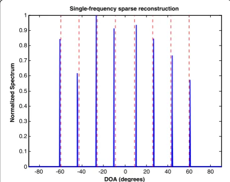
In the first example, sparse signal reconstruction is ap-plied under single frequency operation to perform DOA estimation. Since the difference co-array has eight posi-tive lags, sparse reconstruction can be applied to resolve up to eight sources. A total of eight BPSK sources, uni-formly spaced between −60° and 60°, are considered. The number of snapshots used is 1,000. Spatially and temporally white Gaussian noise is added to the observa-tions, and the SNR is set to 10 dB for all sources. The search space is discretized uniformly between −90° and 90° with a 0.2° step size, and the regularization param-eter λt, is empirically chosen as 0.7 in this example. The
normalized spectrum obtained using sparse signal recov-ery is shown in Figure 5. The dashed vertical lines in the figure indicate the true source directions. A small bias can be noticed in the estimates, and the root mean squared error (RMSE), computed across the angles of arrival, is found to be 1.05°in this case.
In the second example, sparse reconstruction is ap-plied under dual-frequency operation. The physical co-prime array is now operated at both frequencies ω0
-20 -15 -10 -5 0 5 10 15 20 Coarray element location (×λ0/2)
Difference coarray at ω0
Difference coarray at ω1
Figure 8Dual frequency combined difference co-array.ω1= 2ω0.
-80 -60 -40 -20 0 20 40 60 80
0 0.1 0.2 0.3 0.4 0.5 0.6 0.7 0.8 0.9 1
Dual-frequency sparse reconstruction
DOA (degrees)
Normalized Spectrum
Figure 9Dual-frequency sparse reconstruction.D= 13 sources.
-80 -60 -40 -20 0 20 40 60 80
0 0.1 0.2 0.3 0.4 0.5 0.6 0.7 0.8 0.9 1
Dual-frequency sparse reconstruction
DOA (degrees)
Normalized Spectrum
Figure 7Dual-frequency sparse reconstruction.D= 11 sources. -10 -8 -6 -4 -2 0 2 4 6 8 10
Coarray element location (×λ0/2)
Difference coarray at ω0
Difference coarray at ω1
and ω1= 8/9ω0. Sources with proportional spectra are
assumed, and thus, the single measurement vector for-mulation of Section 3 can be used. The combined dif-ference co-array is shown in Figure 6. It has a total of 33 unique lags, which makes it capable of resolving up to 16 sources, theoretically. However, this number is not achievable because of the high mutual coherence of the dictionary. Since some of the virtual sensors in the combined co-array are closely separated, leading to highly correlated observations, deterioration in per-formance is observed if the number of sources is in-creased beyond 11. We consider 11 BPSK sources with proportional spectra, which are uniformly spaced be-tween −75° and 75°. The SNR is set to 10 dB for the sources at the two frequencies, and the total number of snapshots is equal to 2,000. The regularization param-eter λt is set to 0.25, and the search space is divided
into 181 bins of size 1°. Figure 7 shows the normalized spectrum obtained using this method. It is evident that all the sources are correctly resolved. The RMSE in this example is equal to 0.84°. A different choice of the two operational frequencies may reduce the mutual coherence, thereby permitting a larger number of sources to be esti-mated. For illustration, the second frequency is now set to
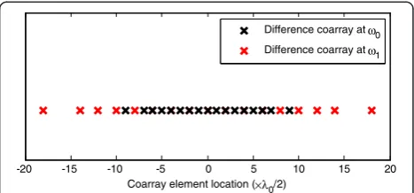
ω1= 2ω0. By choosing a frequency which is an integer
multiple ofω0, the combined co-array positions are
guar-anteed to be integer multiples ofd0. As a result, the
mini-mum separation between two consecutive co-array elements is equal tod0. The combined difference co-array
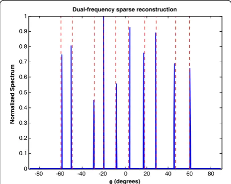
is shown in Figure 8. The co-array has 13 unique positive lags, which means that the maximum number of resolv-able sources is equal to 13. This is tested by considering 13 uniformly spaced sources between −75° to 75°. The SNR is again set to 10 dB, and the number of snap-shots is set to 2,000. The regularization parameter is again set to 0.25, and the search space is divided into 181 angle bins. Figure 9 shows the normalized spectrum using the dual-frequency sparse reconstruction method. It is
evident that all the sources are correctly estimated. The RMSE is found to be 0.26°in this case.
In the following example, the entire array is operated atω0, but only the elements at [2d04d09d0] also operate
at the second frequency ω1= 2ω0. The combined
ence co-array is shown in Figure 10, where the differ-ence co-array atω0is shown in black; and the additional
lags, obtained by operating the subarray atω1, are shown
in red. The overall difference co-array has ten positive lags which imply that up to ten sources can be resolved. This is tested by considering ten sources with respective DOAs [−60°, −49°, −29°, −20°, −9°, 3°, 18°, 29°, 47°, 60°]. The number of snapshots is set to 2,000 at each fre-quency, and the SNR is 10 dB. The regularization par-ameter is set to 0.7 in this example, and the search space is kept the same. Figure 11 shows the normalized spectrum using the dual-frequency sparse reconstruction method. It can be noticed that all the sources are cor-rectly estimated, and the corresponding RMSE is 0.86°.
-15 -10 -5 0 5 10 15
Coarray element location (×λ
0/2)
Difference coarray at ω
0
Difference coarray at ω
1
Figure 10Dual frequency combined difference co-array.ω1= 2ω0.
-80 -60 -40 -20 0 20 40 60 80
0 0.1 0.2 0.3 0.4 0.5 0.6 0.7 0.8 0.9 1
θθθθ (degrees)
Normalized Spectrum
Dual-frequency sparse reconstruction
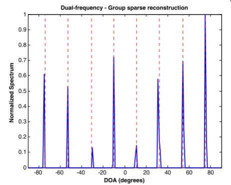
The following example examines the case when sources have nonproportional spectra. In this case, group sparse reconstruction is applied. The two operational frequencies are selected to beω0and 2ω0. Eight sources with
nonpro-portional spectra are considered. The SNR of all the sources at the first frequency is set to 10 dB. At the second frequency, the SNR of each source is a realization of a uni-formly distributed random variable between 5 and 15 dB. This ensures that the sources have nonproportional spec-tra. The noise variance is set to unity at the two frequen-cies, and a total of 2,000 snapshots are used. Figure 12 shows the normalized spectrum obtained using the for-mulation in Section 3 which mistakenly assumes propor-tional source spectra. Consequently, this method is expected to fail as evident in the spectrum of Figure 12. One of the sources is not resolved and several spurious
peaks appear in the spectrum. The DOA estimation is next repeated using group sparse reconstruction which was discussed in Section 4. This method does not require the sources to have proportional spectra. The mean of the recovered spectra at the two employed frequencies is computed and shown in Figure 13. It can be seen that group sparse reconstruction is successful in localizing the DOAs of all the sources. The RMSE is found to be 0.6°in this case.
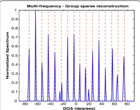
The next example confirms the increase in the number of resolvable sources by using group sparse reconstruction compared to the single-frequency sparse reconstruction. As stated in the first example, the maximum number of re-solvable sources using single-frequency sparse reconstruc-tion is equal to the number of unique positive lags in the difference co-array, which is eight in this case. A total of 16 sources with nonproportional spectra is considered in the
-80 -60 -40 -20 0 20 40 60 80
0 0.1 0.2 0.3 0.4 0.5 0.6 0.7 0.8 0.9 1
Multi-frequency - Group sparse reconstruction
DOA (degrees)
Normalized Spectrum
Figure 14Multi-frequency group sparse reconstruction.D= 16 sources with nonproportional spectra.
-80 -60 -40 -20 0 20 40 60 80
0 0.1 0.2 0.3 0.4 0.5 0.6 0.7 0.8 0.9 1
Single-frequency - Sparse reconstruction
DOA (degrees)
N
o
rm
al
iz
ed
S
p
ect
ru
m
Figure 15Single-frequency sparse reconstruction.D= 16 sources.
-80 -60 -40 -20 0 20 40 60 80
0 0.1 0.2 0.3 0.4 0.5 0.6 0.7 0.8 0.9 1
Dual-frequency - Group sparse reconstruction
DOA (degrees)
Normalized Spectrum
Figure 13Dual-frequency group sparse reconstruction.D= 8 sources with nonproportional spectra.
example. The sources are uniformly spaced between−75°
and 75°. Twenty uniformly spaced frequencies betweenω0
and 2ω0are employed. The SNR of each source at each
frequency is chosen randomly between−5 and 5 dB, and the number of snapshots at each frequency is set to 1,000. Figure 14 shows the normalized mean spectrum obtained using group sparse reconstruction. It can be seen that all the sources are correctly estimated, and the RMSE is equal to 0.35° in this case. Figure 15 shows the normalized spectrum for the single-frequency sparse reconstruction case. This figure confirms that sparse reconstruction using a single frequency completely fails in estimating the sources. This is due to the fact that single-frequency sparse reconstruction can only resolve up to eight sources which is smaller than the total number of sources in this example.
The final example examines the case where the source signals have overlapping spectra but do not share the same bandwidth. Group sparse reconstruction can still be used to perform DOA estimation. Thirty percent of the source powers at the employed frequencies in the pre-vious example are randomly set to zero. The remaining parameters are kept the same. Figure 16 shows the nor-malized spectrum using group sparse reconstruction. It is evident that all sources are correctly estimated. Some spurious peaks are present in the spectrum, and an in-crease in the estimates bias is obtained. The RMSE is found to be 0.61°.
6 Conclusions
A sparse reconstruction method has been proposed for DOA estimation using multi-frequency co-prime arrays. The proposed approach offers an enhancement in the de-grees of freedom over the single-frequency co-prime array. For sources with proportional spectra, all observations at
the employed frequencies are combined to form a received signal vector at a larger virtual array, whose elements are given by the combination of the difference co-arrays at the individual frequencies, thereby increasing the number of resolvable sources. In the case of sources with nonpropor-tional spectra, the common support that is shared by the observations at the employed frequencies is exploited through group sparse reconstruction. Although the offered degrees of freedom are less than those of the multi-frequency approach for proportional spectra, they exceed those offered by single-frequency co-prime array with sparse reconstruction. Numerical examples demonstrated the superior performance of the proposed multi-frequency approach compared to its single-frequency counterpart.
Abbreviations
CoSaMP:Compressive sampling matched pursuit; DFT: Discrete fourier transform; DOA: Direction of arrival; DOF: Degree of freedom; Lasso: Least absolute shrinkage and selection operator; MHA: Minimum hole array; MRA: Minimum redundancy array; OMP: Orthogonal matching pursuit; RMSE: Root mean squared error; SNR: Signal-to-noise ratio; ULA: Uniform linear array.
Competing interests
The authors declare that they have no competing interests.
Acknowledgements
This work was supported by the Office of Naval Research (ONR) under grant N00014-13-1-0061.
Received: 8 July 2014 Accepted: 9 October 2014 Published: 27 November 2014
References
1. HL Van Trees,Optimum Array Processing: Part IV of Detection, Estimation, and Modulation Theory(John Wiley and Sons, New York, 2002)
2. S Chandran,Advances in Direction-of-Arrival Estimation(Artech House, Norwood, MA, 2006)
3. TE Tuncer, B Friedlander,Classical and Modern Direction-of-Arrival Estimation
(Academic Press (Elsevier), Boston, MA, 2009)
4. R Schmidt, Multiple emitter location and signal parameter estimation. IEEE. Trans. Antenn. Propag.34(3), 276–280 (1986)
5. R Roy, T Kailath, ESPRIT-Estimation of signal parameters via rotational invariance techniques. IEEE. Trans. Acoust. Speech. Signal. Process.37(7), 984–995 (1989) 6. A Moffet, Minimum-redundancy linear arrays. IEEE. Trans. Antenn. Propag.
16(2), 172–175 (1968)
7. GS Bloom, SW Golomb, Application of numbered undirected graphs. Proc. IEEE65(4), 562–570 (1977)
8. C Chambers, TC Tozer, KC Sharman, TS Durrani, Temporal and spatial sampling influence on the estimates of superimposed narrowband signals: when less can mean more. IEEE Trans. Signal Process.44(12), 3085–3098 (1996) 9. WK Ma, TH Hsieh, CY Chi, inProceedings of the IEEE International Conference
on Acoustics, Speech and Signal Processing (ICASSP), 2009. DOA estimation of quasi-stationary signals via Khatri-Rao subspace (Taipei, Taiwan, 2009),
pp. 2165–2168
10. DH Johnson, DE Dudgeon,Array Signal Processing: Concepts and Techniques
(Prentice Hall, Englewood, NJ, 1993)
11. RT Hoctor, SA Kassam, The unifying role of the coarray in aperture synthesis for coherent and incoherent imaging. Proc. IEEE78(4), 735–752 (1990) 12. P Pal, PP Vaidyanathan, Nested arrays: a novel approach to array processing with
enhanced degrees of freedom. IEEE Trans. Signal Process.58(8), 4167–4181 (2010) 13. PP Vaidyanathan, P Pal, Sparse sensing with co-prime samplers and arrays.
IEEE Trans. Signal Process.59(2), 573–586 (2011)
14. SU Pillai, Y Bar-Ness, F Haber, A new approach to array geometry for improved spatial spectrum estimation. Proc. IEEE73(10), 1522–1524 (1985)
-80 -60 -40 -20 0 20 40 60 80
Multi-frequency - Group sparse reconstruction
DOA (degrees)
Normalized Spectrum
15. P Pal, PP Vaidyanathan, inProceedings of the Digital Signal Processing Workshop and IEEE Signal Processing Education Workshop (DSP/SPE). Coprime sampling and the MUSIC algorithm (Sedona, AZ, 2011), pp. 289–294 16. YI Abramovich, DA Gray, AY Gorokhov, NK Spencer, Positive-definite Toeplitz
completion in DOA estimation for nonuniform linear antenna arrays. I. Fully augmentable arrays. IEEE Trans. Signal Process.46(9), 2458–2471 (1998) 17. YI Abramovich, NK Spencer, AY Gorokhov, Positive-definite Toeplitz
completion in DOA estimation for nonuniform linear antenna arrays. II. Partially augmentable arrays. IEEE Trans. Signal Process.47(6), 1502–1521 (1999) 18. E BouDaher, Y Jia, F Ahmad, M Amin, inProceedings of the 22nd European
Signal Processing Conference (EUSIPCO), 2014. Direction-of-arrival estimation using multi-frequency co-prime arrays (Lisbon, Portugal, 2014)
19. F Ahmad, SA Kassam, Performance analysis and array design for wide-band beamformers. J. Electron. Imag.7(4), 825–838 (1998)
20. JL Moulton, SA Kassam, inProceedings of the 43rd Annual Conference on Information Sciences and Systems. Resolving more sources with multi-frequency coarrays in high-resolution direction-of-arrival estimation (Baltimore, MD, 2009), pp. 772–777
21. YD Zhang, MG Amin, B Himed, inProceedings of the IEEE International Conference on Acoustics, Speech and Signal Processing (ICASSP), 2013. Sparsity-based DOA estimation using co-prime arrays (Vancouver, Canada, 2013), pp. 3967–3971
22. P Pal, PP Vaidyanathan, inProceedings of the 2012 Conference Record of the Forty Six Asilomar Conference on Signals, Systems and Computers (ASILOMAR). On application of LASSO for sparse support recovery with imperfect correlation awareness ( Pacific Grove, CA, 2012), pp. 958–962 23. TJ Shan, M Wax, T Kailath, On spatial smoothing for direction-of-arrival
estimation of coherent signals. IEEE. Trans. Acous. Speech. Signal. Process. 33(4), 806–811 (1985)
24. N Hu, Z He, X Xu, M Bao, DOA estimation for sparse array via sparse signal reconstruction. IEEE. Trans. Aerospace. Electron. Syst.49(2), 760–773 (2013) 25. H Wang, M Kaveh, Coherent signal-subspace processing for the detection
and estimation of angles of arrival of multiple wide-band sources. IEEE. Trans. Acoust. Speech. Signal. Process.33(4), 823–831 (1985)
26. Y Yoon, LM Kaplan, JH McClellan, TOPS: New DOA estimator for wideband signals. IEEE Trans. Signal Process.54(6), 1977–1989 (2006)
27. Z Tan, A Nehorai, Sparse direction of arrival estimation using co-prime arrays with off-grid targets. IEEE. Signal. Process. Lett.21(1), 26–29 (2014) 28. D Malioutov, M Cetin, A Willsky, Sparse signal reconstruction perspective for
source localization with sensor arrays. IEEE Trans. Signal Process. 53(8), 3010–3022 (2005)
29. R Tibshirani, Regression shrinkage and selection via the Lasso. J. Roy. Stat. Soc Ser. B.58(1), 267–288 (1996)
30. JA Tropp, AC Gilbert, Signal recovery from random measurements via orthogonal matching pursuit. IEEE. Trans. Informat. Theory.53(12), 4655–4666 (2007) 31. D Needella, JA Tropp, CoSaMP: iterative signal recovery from incomplete and
inaccurate samples. Appl. Comput. Harmonic. Analysis.26(3), 301–321 (2009) 32. VA Morozov, On the solution of functional equations by the method of
regularization. Soviet. Math. Doklady.7, 414–417 (1966)
33. M Davenport, M Duarte, Y Eldar, G Kutyniok,Compressed Sensing: Theory and Applications(Cambridge University Press, Cambridge, UK, 2012), p. 1 34. M Yuan, Y Lin, Model selection and estimation in regression with grouped
variables. J. Roy. Stat. Soc. Ser. B.68(1), 49–67 (2007)
35. Y Eldar, P Kuppinger, H Bolcskei, Block-sparsity signals: uncertainty relations and efficient recovery. IEEE Trans. Signal Process.58(6), 3042–3054 (2010)
doi:10.1186/1687-6180-2014-168
Cite this article as:BouDaheret al.:Sparse reconstruction for direction-of-arrival estimation using multi-frequency co-prime arrays.EURASIP Journal on Advances in Signal Processing20142014:168.
Submit your manuscript to a
journal and benefi t from:
7Convenient online submission 7Rigorous peer review
7Immediate publication on acceptance 7Open access: articles freely available online 7High visibility within the fi eld
7Retaining the copyright to your article