Semiparametric quasi-likelihood estimation with missing data

This is a repository copy of Semiparametric quasi-likelihood estimation with missing data

.

White Rose Research Online URL for this paper:

http://eprints.whiterose.ac.uk/100152/

Version: Accepted Version

Article:

Bravo, Francesco orcid.org/0000-0002-8034-334X and Jacho-Chavez, David T. (2016)

Semiparametric quasi-likelihood estimation with missing data. Communications in

Statistics, Theory and Methods. pp. 1345-1369. ISSN 0361-0926

https://doi.org/10.1080/03610926.2013.863928

[email protected] https://eprints.whiterose.ac.uk/

Reuse

Items deposited in White Rose Research Online are protected by copyright, with all rights reserved unless indicated otherwise. They may be downloaded and/or printed for private study, or other acts as permitted by national copyright laws. The publisher or other rights holders may allow further reproduction and re-use of the full text version. This is indicated by the licence information on the White Rose Research Online record for the item.

Takedown

If you consider content in White Rose Research Online to be in breach of UK law, please notify us by

Semiparametric Quasi-likelihood Estimation with Missing Data

Francesco Bravo

University of York

David T. Jacho-Ch´

avez

Emory University

Abstract

This paper develops quasi-likelihood estimation for generalized varying coefficient partially linear models when the response is not always observable. The paper considers two estimation methods and shows that under the assumption of selection on the observables the resulting estimators are asymptotically normal. As an application of these results the paper proposes a new estimator for the average treatment effect parameter. A simulation study illustrates the finite sample properties of the proposed estimators.

Keywords: Backfitting; Double Robustness; Inverse Probability Weighting; Profiling; Unconfoundness.

JEL classification: C13; C14; C21

1

Introduction

Quasi-likelihood estimation is routinely used in econometrics and statistics to estimate known index structure models for binary, counts and fractional responses, see for example McCullagh & Nelder (1989), Gourieroux, Monfort & Trognon (1984) and especially Wooldridge (2010) for a comprehensive review of models and applica-tions). Quasi-likelihood estimation can also be used in the context of semiparametric regression models and in particular for generalized varying coefficients partially linear models. These models are semiparametric exten-sions of the classical generalized linear models and include many important semiparametric regression models such as the kernel generalized linear model of Fan, Heckman & Wand (1995), the generalized partially linear model of Carroll, Fan, Gijbels & Wand (1997), and the varying-coefficient model of Hastie & Tibshirani (1993) and of Cai, Fan & Li (2000). Compared to the popular partially linear model considered by Engle, Granger, Rice & Weiss (1986) and Robinson (1988) generalized varying partially linear models offer additional flexibility and allow interaction effects between covariates and the nonparametric components while avoiding the curse of dimensionality typically associated with partially linear models. Furthermore as with classical (i.e. parametric) generalized linear models using a canonical link function ensures that the final estimates have always the correct range (e.g. Logit link leads to a probability), however as opposed to classical generalized linear models the choice of the link function is less important, making them therefore more robust to potential misspecification of the conditional mean.

In this paper we consider quasi-likelihood estimation for generalized varying coefficients partially linear models when the responses are partially observable. Under the assumption of selection on the observables we propose a new estimator for the unknown parameters based oninverse probability weighting method (Horvitz & Thompson 1952). This method has been used for regression models with missing data, see for example Robins, Rotnitzky &

∗_{Department of Economics, University of York, Heslington, York YO10 5DD, UK. E-mail: [email protected]. Web}

Page: https://sites.google.com/a/york.ac.uk/francescobravo/.

†_{Department of Economics, Emory University, Rich Building 306, 1602 Fishburne Dr., Atlanta, GA 30322-2240, USA. E-mail:}

Zhao (1994) and Robins & Rotnitzky (1995), in the treatment effect literature, see for example Hirano, Imbens & Ridder (2003), in nonclassical measurement error models, see for example Robins, Hsieh & Newey (1995) and Chen, Hong & Tamer (2005), attrition in panel data, see for example Wooldridge (2002), and by Wooldridge (1999) and Wooldridge (2007) forM-estimation with missing data. The probabilities of the weighting method are typically unknown and therefore have to be estimated either with parametric or with nonparametric methods. In this paper we consider the parametric approach because as opposed to the nonparametric one it does not suffer from the curse of dimensionality and it is less negatively affected by a high proportion of missing data in the sample, making it perhaps more useful from an empirical point of view. Furthermore, as noted by Wooldridge (2007), as long as the conditional mean is correctly specified and the assumption of selection on the observables holds misspecification of the parametric estimator for probabilities does not cause inconsistency of the weighted estimator for the parameters of the generalized varying coefficient partially linear estimator.

The results of this paper are rather general and can be seen as a semiparametric extension of some of the results obtained by Wooldridge (2007). The results are based on backfitting and profiling, which are the two main approaches to estimate parameters for general semiparametric models and differ in the way they deal with the infinite dimensional parameter. To be specific, backfitting involves iterating between the estimation of the infinite dimensional parameter and that of the finite dimensional one until convergence, see for example Hastie & Tibshirani (1990), Mammen, Linton & Nielsen (1999) and Opsomer (2000). Profiling involves reparameterizing the infinite dimensional parameter as a certain function of the finite dimensional parameter and then estimate simultaneously the resulting reparameterized infinite dimensional parameter as well as the finite dimensional one, see for example Severini & Staniswalis (1994), Murphy & Van der Vaart (2000) and Lam & Fan (2008). A similar procedure, albeit without reparameterization is considered by Ai & Chen (2003) for semiparametric moment conditions models. Opsomer & Ruppert (1999) and more recently Van Keilegom & Carroll (2007) compare backfitting and profiling and note that in certain situations they result in asymptotically equivalent estimators as long as different level of smoothing is applied.

The new results of the paper are the following: First we show that the proposed estimators defined as the solutions to a set of local quasi-scores are consistent. This result is based on a generalization to infinite dimensional parameters of the same approach used by Foutz (1977), and complements the standard approach based on the global concavity of the quasi-likelihood function. Second, we show that both backfitting and profiling lead to estimators that are asymptotically normal but they are not asymptotically equivalent even if we consider different level of smoothing. Third, as an application of these results we propose a new semiparametric estimator for the average treatment effect parameter. This new estimator is motivated by some recent literature in health economics (see e.g. Basu, Polsky & Manning (2008) and references therein) advocating the use of parametric generalized linear models to capture potential nonlinear effects and interactions between outcomes and covariates as well as specific structures of the outcomes. Our estimator is flexible enough to capture these important features while preserving some of the advantages of using parametric methods. Furthermore for Normal, Bernoulli and Poisson quasi-likelihoods the new estimator enjoys the so-called doubly-robust property as noted by Wooldridge (2007). Finally we use simulations to investigate the finite sample properties of the estimators based on backfitting and profiling and for the new average treatment effect estimator. The latter are compared with those based on commonly used alternatives.

maximum in models with an infinite dimensional parameters.

The rest of the paper is structured as follows: Section2 introduces the basic model and discusses the two general estimation approaches. Section 3 contains the main theoretical results. Section 4 considers average treatment effect estimation and proposes a novel estimator based on the results of the previous sections. Section

5illustrates the results with three examples and related simulations. Finally Section6contains some concluding remarks. An Appendix contains all the proofs.

2

The Model and the Estimators

The model we consider is a generalized varying coefficient partially linear model (GVCPL henceforth)

E(Y|X) =g−1_[X⊤

1 β0+X2⊤α0(X3)], (1)

where g−1_{(·) is the inverse function of the known link function g(·), X}

1 andX2 are respectively a k1 and k2 -dimensional vectors,β0 is a vector of unknown parameters,α(·) is a vector of unknown smooth functions, and

X3 is a scalar covariate. GVCPL includes a number of important semiparametric regression models including the kernel generalized linear model of Fan et al. (1995) (specification (1) withoutX1,X2, andβ), the generalized partially linear model of Carroll et al. (1997) (specification (1) withX2 = 1), the varying-coefficient model of Hastie & Tibshirani (1993) and of Cai et al. (2000) (specification (1) withoutX1 andβ).

Let W⊤

i = Yi, Xi⊤

(i= 1, ..., n) denote an i.i.d. sample from W⊤ _{= Y, X}⊤_{; when the response Y}

i is

always observable the unknown parameters in (1) can be estimated by the same quasi-likelihood approach used by Severini & Staniswalis (1994), Fan et al. (1995), Carroll et al. (1997) and many others. To be specific, let

Q g−1_{(·), Ydenote a quasi-likelihood that is defined by}

∂Q(µ, Y)

∂µ =

Y −µ V(µ),

where the variance function V(·) is known and may depend on an unknown scale parameter σ2 _{(see e.g.} Mc-Cullagh & Nelder (1989) for examples), and let

α0j(v) =aj+bj(v−u) j= 1, ..., k2

forv in a neighbourhood ofuandaj =αj(u),bj =α′j(u) denote a linear1approximation forαj(v). Then for

a fixedx3

Qn(β, α, x3) :=

n

X

i=1

Qg−1 X1⊤iβ+X2⊤i(a+b(X3i−x3)), YiKh1(X3i−x3) , (2)

where defines a local quasi-likelihood function that can be used to estimate α0(·) and β0 using either the backfitting or profiling method. If however, some of the responses are missing and this fact is not taken into account into the estimation process, both approaches might result in inconsistent estimators.

We characterize missing data with a binary indicatorT ={0,1} so that we have an i.i.d. sample W⊤

i , Ti

from W⊤_{, Tand the Y}

i are not observed if Ti is zero. The key of our results is that the covariates are good

predictors of the selection as the following assumption specifies:

S1 The vectorW is always observed when T= 1;

1_{The results of the paper can be easily extended to the case of a polynomial approximation. The only change would be in} LemmaA.1inAppendix Ain which the order of approximation would change toh(p+1)q _{wherepis the degree of the polynomial}

S2 (i)Y ⊥T|X, (ii) 0<Pr (T = 1|X)≤1.

Assumption S2(i) corresponds to the missing at random in the statistical literature, and it is related to the so-called unconfoundness in the programme evaluation literature. A fundamental implication of S2 is that if the selection probabilities π(Xi) were known, then the generalized varying coefficient partially linear model

specification (1) for the missingY’s can be recovered by weighting the selected observations by the inverse of the probability of selection. This suggests the following inverse probability weighting (IPW henceforth) modification of (2)

Qn(β, α,bπ, x3) :=

n

X

i=1

Ti

b

π(Xi)Q

g−1 X1⊤iβ+X2⊤i(a+b(X3i−x3)), YiKh1(X3i−x3) , (3)

whereKh1(·) =K(·/h1),K(·) is a kernel function,h1=:h1(n) is the bandwidth and thebπ(Xi)’s are consistent estimates of the typically unknown selection probabilitiesπ(Xi). Also let

Qn(β, α,πb) := n

X

i=1

Ti

b

π(Xi)

Qg−1 _X⊤

1iβ+X2⊤iα(X3i), Yi (4)

denote the inverse probability weighting quasi-likelihood.

The estimation of the unknownα0(·) andβ0is based on both (3) and (4), and can be carried out using either the backfitting or profiling algorithm. The estimators can be defined either as maximizers of (3) and (4) or as the solutionβband α_bto the quasi-score equations defined by the first order conditions from (3) and (4), that is

∂Qn(β, α,π, xb 3)/∂(β⊤, a⊤, b⊤)⊤ = 0, (5)

∂Qn(β,α,b bπ)/∂β= 0.

The results of the paper are valid for both cases and with simple modifications in the proofs also for estimators

b

β andαb defined as the solution of

n

X

i=1

Ti

b

π(Xi)

ϕ Yi;X1⊤iβ+X2⊤i(a+b(X3i−x3)) hX1⊤i, X2⊤i⊗[1,(X3i−x3)]⊤Kh1(X3i−x3)

i⊤ = 0,

n

X

i=1

Ti

b

π(Xi)ϕ Yi;X

⊤

1iβ+X2⊤iαb

X1i= 0,

where ϕis a known scalar function. In what follows we consider the case of estimators defined as solution to quasi-score equations (5).

2.1

Backfitting Estimation

The idea of backfitting, often called two-step procedure, is to use first use a set of local first order conditions (5) based on (3) to obtain local estimates of all the unknown parameters, and then to use the global set of first order condition (5) based on (4) to improve the estimation of the finite dimensional parameter. To be specific, the procedure consists of the following steps:

B1 Either find βb, ba and bb that solve the (k1+ 2k2)×1 vector of local first-order conditions ∂Qn(β, α,bπ,

x3)/∂(β⊤, a⊤, b⊤)⊤ = 0, or for a fixed β find ba andbb that solve the 2k2×1 vector of local first-order conditions∂Qn(β, α,bπ, x3)/∂(a⊤, b⊤)⊤= 0;

The above two steps can then be iterated until convergence if needed. Note that the final estimate αbobtained at the end ofB2 can be improved by considering a third-step which involves solving thek2×1 vector of local first-order conditions ∂Qn(β, α,b bπ, x3)/∂a= 0. Unless the functions αare of particular interest, this last step may be omitted.

Backfitting deliversn1/2_{-consistent estimators forβ}

0; however, in order to achieve then1/2-rate, they require undersmoothing (see Theorem (3.2) below for details). To avoid undersmoothing, we propose an alternative method that is computationally more involved.

2.2

Profiling Estimation

The method of profiling, or one-step estimation, is based on the notion of least favourable curve that is defined to be the parameterization αβ(·) of α(·) which has the smallest possible (Fisher) information for β and such

that atβ0,αβ0(·) =α(·). As long as this curve can be estimated, it can be used to compute the least favorable quasi-score forβ, which coincides with the efficient one. The procedure consists of the following steps:

P1 For a given β let αbβ := ba that solve the 2k2 × 1 vector of local first-order conditions

∂Qn(β, αβ,π, xb 3)/∂(a⊤, b⊤)⊤= 0;

P2 Findβbthat solves thek1×1 vector of first-order conditions∂Qn(β,αbβ,πb)/∂β= 0.

It is important to note that the IPW profile quasi-score forβ is

∂Qn(β,αbβ,bπ)

∂β =

n

X

i=1

Ti

b

πi(Xi)

q1 g−1 X1⊤iβ+X2⊤iαbβ(X3i), Yi X1i+

∂αbβ(X3i)

∂β⊤

⊤

X2i

!

,

whereq1(x, y) =∂Q

g−1_{(x), y/∂x. This involves the difficult computation of thek}

2×k1matrix∂αbβ(X3i)/∂β⊤

(the so-called least favorable direction) using, for example, numerical derivatives. To overcome this difficulty we can use as in Severini & Staniswalis (1994) and Lam & Fan (2008) a simple estimator that is based on a local version of its explicit expression (given in (A−22) of the Appendix) that is

∂αbβ(x3)/∂∂β⊤= 1

n

n

X

i=1

Ti

b

πi(Xi)

q2 g−1(X1⊤iβ+X2⊤iαbβ(X3i)), Yi

X2iX2⊤iKh(X3i−x3)

!−1

×

1

n

n

X

i=1

Ti

b

πi(Xi)

q2 g−1(X1⊤iβ+X2⊤iαbβ(X3i)), Yi

X2iX1⊤iKh(X3i−x3) ,

whereq2(x, y) =∂2Q

g−1_{(x), y/∂x}2_{; see Section4for further details on the computation of this estimator.}

3

Main Results

We begin this section by introducing some auxiliary notation and the following convention: A quantity with a superscript π indicates that the relevant expectation is weighted by the inverse of the propensity score, so for example ∆ (x) = E[g(x)] and ∆π(x) = E[g(x)/π(x)]. For j = 0,1, . . .let qj(x, y) = ∂jQ

g−1_{(x), y/∂x}j_,

ρj(x) = ∂g−1(x)/∂x j

/var (y|x),κj =R tjK(t)dt, υj =RtjK2(t)dt andη =X1⊤β+X2⊤α(X3). Let B(β0) denote an open neighbourhood ofβ0; and assume that:

A2 The functions α′′

j(·) (j= 1, . . . , k2) are continuous in X3; the functionsV (·) and g(·) are, respectively, twice and three times continuously differentiable inB(β0);

A3 The matricesEq2

1(η, Y)XjXk⊤|X3=x3(j, k= 1,2) are twice continuously differentiable inx3∈ X3; the least favourable curveαβ(·) is three times continuously differentiable inx3∈ X3andB(β0);

A4 The matrices Eρ2(η0)XjXj⊤|X3=x3 (j= 1,2) are nonsingular, E{ρ2(η0)XjXj⊤|X3 =x3} are nega-tive definite for each x3 ∈ X3, E

ρ2(η0)XjXj⊤

are negative definite, and for some γ > 0,

E[kT q1(η0, Y)X1⊤, X2⊤

⊤

/π(X)k2+γ] < ∞ , E[kρ2(η0)XjXj⊤k

2+γ

] < ∞,

E[kρ2(η0)XjXj⊤k

2+γ

|X3 = x3] < ∞, E[supx3∈X3,β∈B(β0)kq3(η)XjX ⊤

j Xjl k] < ∞, (j = 1,2, l =

1, . . . , k=k1+k2);

A5 The kernelK is a bounded symmetric density function with bounded support.

Assumptions A1-A5 are standard moment and smoothness conditions in the literature on nonparamet-ric/semiparametric estimation with quasi-likelihood functions, see e.g. Severini & Staniswalis (1994), Carroll et al. (1997) and Cai et al. (2000). Note that we do not require the quasi-likelihood to be globally concave and thus we allow for possible misspecification of the variance. These conditions ensure the consistency and asymptotic normality of a unique solution to the quasi-score equations (5).

The computation of bπ(Xi) can be done using binary maximum likelihood under the following additional

standard regularity conditions. Let π(X, γ) denote a parametric model for π(X) where γ ∈ Γ ⊂ Rdγ, and assume that

A6 (i)π(X, γ)>0 for allXand allγ∈Γ, (ii)π(X, γ0) =π(X), (iii)bγhas the following stochastic expansion:

n1/2(bγ−γ0) =I−1(γ0) 1

n1/2

n

X

i=1

∂πi(γ0)

∂γ

(Ti−πi(γ0))

πi(γ0) (1−πi(γ0))

+op(1) .

Let

Σ (α, β, x3) =E

ρ2(X1⊤β+X2⊤α(X3))[X1⊤, X2⊤]⊤

X⊤ 1, X2⊤

|X3=x3 , Γ (α, β, x3) =E

ρ2(X1⊤β+X2⊤α(X3))[X1X2⊤, X2X2⊤]⊤α′′(X3)|X3=x3 .

The following theorem establishes the asymptotic distribution of the local estimators used in the backfitting procedure described in stepB1.

Theorem 3.1 _{Under S1,S2andA1-A6. Then}

(nh1)1/2

" b

β−β0

b

α(x3)−α0(x3)

!

−h

2

1b1(α0, β0, x3) 2

#

d

→N

"

0 0

#

,v0A(β0, α0, π, x3) f(x3)

!

,

where

b1(α, β, x3) =κ2Σ (α, β, x3)−1Γ (α, β, x3),

A(β, α, π, x3) = Σ (α, β, x3)−1Σπ(α, β, x3) Σ (α, β, x3)−1.

Forj, k= 1,2 let

Bjk(α, β, x3) =E

ρ2 X1⊤β+X2⊤α(X3)

XjXk⊤|X3=x3

,

Bjk(α, β) =E

ρ2 X1⊤β+X2⊤α(X3)

XjXk⊤

,

D(α, β, x3) =B11π(α, β, x3)B11(α, β, x3)−1B12(α, β, x3) ∆ (α, β, x3)B21(α, β, x3)−

B12(α, β, x3) ∆ (α, β, x3) ,

∆ (α, β, x3) =B22(α, β, x3)−B21(α, β, x3)B11(α, β, x3)−1B12(α, β, x3).

The following theorem establishes then1/2_{-consistency ofβbobtained in stepB2.}

Theorem 3.2 _{Under S1,S2andA1-A6. Ifnh}4_{1→0, then}

n1/2(βb−β0)

d

→N 0, Bb(α0, β0, π),

where

Bb_(α

0, β0, π) =B11(α0, β0)−1Ωb(α0, β0, π)B11(α0, β0)−1,

Ωb(α0, β0, π) =B11π(α0, β0) +E[D(α, β, X3)] +E[D(α, β, X3)]⊤+

EhB12(α0, β0, X3)SαΣκ(α0, β0, X3)−1×

Σπ(α0, β0, X3) Σκ(α0, β0, X3)−1Sα⊤B12(α0, β0, X3)⊤

i

,

whereSα= [0, I,0]andΣκ(α0, β0, x3) =diag[Σ (α, β, x3), κ2B22(α, β, x3)].

Theorem 3.2shows that to achieven1/2_{-consistency using the backfitting method we need to undersmooth.} This is typical for a number of semiparametric models as noted for example by Van Keilegom & Carroll (2007). Note that if one is interested in α0, then because of the undersmoothing it might be desirable to consider a third estimation which uses βb found in step B2, and is defined by the local quasi-score equations

∂Qn(β, α,b bπ, x3))/∂(a⊤, b⊤)⊤= 0. Note also that sinceβbisn1/2-consistent this estimation can be carried out as ifβ was known. This result is summarized in the following theorem. Let

Φ (α, β, x3) =Eρ2(X1⊤β+X2⊤α(X3))[X2X2⊤,0⊤]⊤α′′(X3)|X3=x3, Ψκ(α, β, x3) = diag [B22(α, β, x3), κ2B22(α, β, x3)] ,

Ψυ(α, β, x3) = diag [υ0B22(α, β, x3), υ2B22(α, β, x3)] .

Theorem 3.3 _{Under S1-S2andA1-A6. Then}

(nh2)1/2

" b

α(x3)−α0(x3)

h2(αb′(x3)−α′0(x3))

!

−h

2 2

2 b2(α, β, x3)

#

d

→N

"

0 0

#

,C(α0, β0, x3) f(x3)

!

,

where

b2(α, β, x3) =κ2Ψκ(α, β, x3)−1Φ (α, β, x3),

C(α, β, x3) = Ψκ(α, β, x3)−1Ψπυ(α, β, x3) Ψκ(α, β, x3)−1.

Theorem 3.4 _{Under S1-S2andA1-A6. Then}

n1/2(βb−β0)

d

→N(0, Bp(α0, β0, π))

where

Bp(α0, β0, π) = Ξ (α0, β0)−1Ωp(α0, β0, π) Ξ (α0, β0)−1,

Ξ (α0, β0) =B11(α0, β0)−E

h

B12(α0, β0, X3)B22(α0, β0, X3)−1B12(α0, β0, X3)⊤

i

,

Ωp(α0, β0, π) =B11π(α0, β0)−E

h

B12π(α0, β0, X3)B22(α0, β0, X3)−1B12(α0, β0, X3)⊤

i

−

EhB12(α0, β0, X3)B22(α0, β0, X3)−1B12π(α0, β0, X3)⊤

i

+

EhB12(α0, β0, X3)B22(α0, β0, X3)−1B22π(α0, β0, X3)B22(α0, β0, X3)−1B12(α0, β0, X3)⊤

i

.

4

Average Treatment Effect Estimation

As an application of the results of the previous section we consider the problem of estimating the average treatment effect parameter, see e.g. Imbens (2004) for a recent review. We propose a novel semiparametric estimator that is a middle ground between the parametric specifications recently used in some health economics literature (see e.g. Basu et al. (2008)) and the fully nonparametric approach of Hahn (1998) and Hirano et al. (2003). The estimator combines the regression adjustment approach with the GVCPL specification of the conditional mean, and enjoy a somewhat stronger version of the same double robustness property noted by Wooldridge (2007), because of the semiparametric specification of the conditional mean of the outcomes as opposed to the fully parametric one proposed by Wooldridge (2007).

We follow the standard potential-outcome notation and useY(1) andY(0) to denote the potential outcome for an experimental unit with and without the treatment, which is indicated by the dummy variableT ∈ {0,1}. We are interested in the average treatment effectparameter2

τ0=E[Y (1)−Y (0)] , (6)

As in Section2let{W⊤

i , Ti}ni=1 be an i.i.d. sample and let

Yi=TiYi(1) + (1−Ti)Yi(0) ,

denote the realized outcome. Assume that

S2∗ _{(i)Y (1), Y (0)⊥T|X, (ii) 0<Pr (T= 1|X)<1;}

S3 E[Y(δ)|X] =g−1 _X⊤

1βδ0+X2⊤αδ0(X3)

forδ= 0,1.

AssumptionsS2∗_{(i) and S3imply thatτ}

0 can be estimated by the sample analogue of the mean regressions difference

τ0=Eg−1 X1⊤β01+X2⊤α10(X3)−g−1 X1⊤β00+X2⊤α00(X3), (7) that is

b

τ= 1

n

n

X

i=1

h

g−1X1⊤iβb1+X2⊤iαb1(X3i)

−g−1X1⊤iβb0+X2⊤iαb0(X3i)

i

, (8)

2_{Although similar results can also be obtained for the so-calledaverage treatment effect on the treated parameter}

where βbδ _andαbδ_{(·) are the solutions to (5) with T}

i/bπi and (1−Ti)/(1−bπi) respectively for δ= 1 andδ= 0

computed using both backfitting and profiling methods. LetSα= [0, I,0],πδ =δπ+ (1−δ) (1−π) and

G1(αδ, βδ) =E

"

∂g−1 _X⊤

1βδ+X2⊤α1(X3)

X1

∂(βδ⊤_{, α}δ⊤₎⊤

#

,

G2(αδ, βδ, X3) =E

"

∂g−1 _X⊤

1βδ+X2⊤α1(X3)

X2

∂(βδ⊤_{, α}δ⊤₎⊤ |X3

#

,

F(αδ, βδ, X3) =SαΣ−κ1(αδ, βδ, X3)Σπδ(αδ, βδ, X3)SαΣκ−1(αδ, βδ, X3).

Theorem 4.1 _{(I) UnderS1,S2}∗_{,S3,A1-A6and if nh}4

1→0 then for the backfitting method

n1/2(bτb−τ0)→d N 0, Vb(α0, β0),

where

Vb_(α

0, β0) = var

g−1 _X⊤

1β01+X2⊤α10(X3)

−g−1 _X⊤

1β00+X2⊤α00(X3)

+

X

δ=1,0

Λb1δ(αδ0, βδ0) + Λb2δ(α0δ, β0δ) + Λb3δ(αδ0, βδ0) + Λ3b⊤δ(αδ0, β0δ) + Λb4δ(α0δ, β0δ) + Λb4⊤δ(αδ0, β0δ)

,

and

Λb1δ(αδ0, β0δ) =G⊤1(αδ0, β0δ)Bb(αδ0, βδ0, πδ)G1(αδ0, β0δ), Λb2δ(αδ0, β0δ) =E

G⊤

2(αδ0, β0δ, X3)F(αδ0, β0δ, X3)G2(αδ0, β0δ, X3)

,

Λb3δ(αδ0, β0δ) =G1(αδ0, βδ0)B11−1(α0, β0)E

−B11πδ(α10, β01, X3)B11−1(α10, β01, X3)B12(α10, β10, X3)× ∆(α10, β01, X3)G2(α10, β10, X3) +B12(α01, β01, X3)∆(α10, β01, X3)G2(α10, β01, X3)

Λb4δ(αδ0, β0δ) =−G1(αδ0, β0δ)B−111(α0, β0)E

B12(α0, β0, X3)F(αδ0, β0δ, X3)G2(αδ0, βδ0, X3)

.

(II) Under S1,S2∗_{,S3andA1-A6, then for the profiling method}

n1/2(bτp−τ0)→d N(0, Vp(α0, β0)),

where

Vp_(α

0, β0) = var

g−1 _X⊤

1β01+X2⊤α10(X3)

−g−1 _X⊤

1β00+X2⊤α00(X3)

+

X

δ=1,0

h

Λp_1δ(αδ0, βδ0) + Λ

p

2δ(α δ

0, β0δ) + Λ

p

3δ(α δ

0, βδ0) + Λ

p⊤ 3δ(α

δ

0, β0δ) + Λ

p

4δ(α δ

0, β0δ) + Λ

p⊤ 4δ(α

δ

0, βδ0)

i

,

and

Λp1δ(αδ0, β0δ) =G⊤1(αδ0, β0δ)Bp(αδ0, β0δ, πδ)G1(αδ0, β0δ), Λ

p

2δ(αδ0, β0δ) = Λ2bδ(αδ0, β0δ), Λp_3δ(αδ0, β0δ) =G⊤1(αδ0, β0δ)Ξ−1(αδ0, β0δ)E

B11πδ(αδ0, β0δ, X3)−B12(αδ0, βδ0, X3)B−221(αδ0, βδ0, X3)×

B21πδ(αδ0, β0δ, X3)B11−1(α10, β01, X3)∆(α10, β01, X3), Λp_4δ(αδ0, β0δ) =G⊤1(αδ0, β0δ)Ξ−1(αδ0, β0δ)E

B12π(α10, β01, X3)−B12(α10, β01, X3)B−221(α10, β10, X3)×

B22π(α10, β01, X3)∆(α10, β10, X3).

5

Numerical Experiments

for which the link functions are given, respectively, by

Normal: g(u) =u, Poisson: g(u) = ln(u), Logit: g(u) = ln u

1−u

.

We first consider two separate cases corresponding toδ= 0 and 1, and then use the same two cases to consider average treatment effect estimation.

For the Normal design, we setX2∼U[−2,2],X3∼U[−2,2] andX1= [X11, X12]⊤ withX11∼U[−1,0] and

X12 ∼U[0,1], where we have used the notation V ∼U[a, b] to denote that V follows an uniform distribution between a and b. We set β1

0 = [β101 , β120]⊤ = [1,3]⊤, β00 = [β100 , β200 ]⊤ = [1,1]⊤, α10(u) = 3 cos (2u), and

α0

0(u) = 3 sin (2u). We also setT =I{X⊤θ0−u >0}, whereI{·}is the standard indicator function that equals one if its argument is true and zero otherwise, X = [X⊤

1, X2, X3]⊤, θ0 = [1/4,1/4,1/4,1/4]⊤ and u follows a standard normal distribution. For this specification the proportion of missing responses is 0.50.

In the Poisson and Logit designs, we setβ1

10 = β100 = 0, β201 = β200 =−1, α10(u) = α00(u) = sin(πu). The binary indicator is set as T = I{X⊤_θ

0−u > 0}, where u is a standard normal as in the previous case but withθ0= [0,1/3,1/3,1/3]⊤. For both designs we set X2∼Beta[2,4],X3∼U[−1,1] andX12∼2×Beta[4,2], whereBeta[a, b] denotes a Beta distribution with shape parametersaandb. For this specification the proportion of missing responses is approximately 0.30. Note also that the average treatment effect parameter τ0 is 0 by construction.

In each of 500 replications we generated n pseudo-random numbers from these three designs for n ∈ {100,200,400}. For δ = 1 and δ = 0, we implement the estimators discussed in Section 2.1 and Section

2.2, using a second order Gaussian kernel with bandwidth chosen by Silverman’s rule-of-thumb and a correctly specified Probit model forπi in each replication.

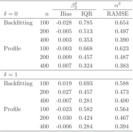
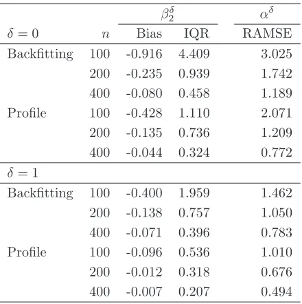
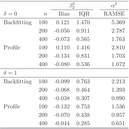
Tables 1, 3 and5 report the median bias (Bias) and the interquartile range (IQR) for the backfitting and profile estimators of βδ

20 - ‘Backfitting’ and ‘Profile’ respectively in the tables. The tables also report the root average mean square error (RAMSE) of the backfitting and profile estimators of the nonparametric component

αδ

0. We first note that all finite sample biases and interquartile range decreases as the sample size increases uniformly across all specifications and designs. More interestingly we observe that the profile estimator of βδ

20 outperforms that based on backfitting across all designs andδs both in terms of absolute median bias and spread in all of the three specifications. The improvement is particularly evident in the case of the Poisson specification, where the finite sample bias of the profile estimator is roughly half that of the backfitting one forδ = 0, and up to 10 times less for δ= 1 and n= 200. The finite sample interquartile range is also considerably smaller especially for n = 100, where it is roughly a quarter for δ = 0 and δ = 1. The profile estimator of αδ

0 also outperforms its backfitting counterpart in terms of RAMSE across all designs and for bothδs.

as in the previous other two cases by the profile estimator in terms of interquartile range. Taken together the results of Tables 1-6 seem to suggest that the proposed estimators perform well in finite samples and can be effectively used in situations where there are missing observations and selection on observables can be assumed.

6

Conclusions

This paper proposes a new estimator for the parameters of generalized varying coefficients partially linear models when the responses are not perfectly observable but selection on the observables can be assumed. The estimator is based on an inverse probability weighting quasi-likelihood method with probability weights calculated using a parametric specification. The resulting estimator enjoys the double robustness property for three important link functions and can be used with many covariates, which makes it very useful from an applied point of view. The paper considers two general estimating techniques, namely backfitting and profiling, which yield estimators that are not asymptotically equivalent. Simulations seems to suggest that the estimators are characterized by good finite sample properties and that the one based on profiling dominates that based on backfitting both in terms of bias and spread.

References

Ai, C. & Chen, X. (2003). Efficient estimation of models with conditional moment restrictions containing unknown functions, Econometrica 71_{: 1795–1843.}

Basu, A., Polsky, D. & Manning, W. (2008). Use of propensity scores in nonlinear response models: The case for health care expenditures. NBER Working paper 14086.

Cai, Z., Fan, J. & Li, R. (2000). Efficient estimation and inference for varying-coefficient models,Journal of the American Statistical Association 95_{: 888–902.}

Carroll, R., Fan, J., Gijbels, I. & Wand, M. (1997). Generalized partially linear single-index models,Journal of the American Statistical Association 92_{: 477–489.}

Chen, J., Fan, J., Li, K. & Zhou, H. (2006). Local quasi-likelihood estimation with data missing at random,

Statistica Sinica16_{: 1071–1100.}

Chen, X., Hong, H. & Tamer, E. (2005). Measurement error models with auxiliary data, Review of Economic Studies72_{: 343–366.}

Engle, R., Granger, C., Rice, J. & Weiss, A. (1986). Nonparametric estimation of the relation between weather and electricity sales, Journal of the American Statistical Association81_{: 310–320.}

Fan, J., Heckman, N. & Wand, M. (1995). Local polynomial kernel regression for generalized linear models and quasilikelihood functions, Journal of the American Statistical Association90_{: 141–150.}

Foutz, R. (1977). On the unique consistent solution to the likelihood equations, Journal of the American Statistical Association72_{: 147–148.}

Gourieroux, C., Monfort, A. & Trognon, A. (1984). Pseudo maximum likelihood methods: Theory,Econometrica

52_{: 681–700.}

Hastie, T. & Tibshirani, R. (1990). Generalized Additive Models, Chapman and Hall.

Hastie, T. & Tibshirani, R. (1993). Varying-coefficient models,Journal of the Royal Statistical Society B55_{: 757–}

796.

Hirano, K., Imbens, G. & Ridder, G. (2003). Efficient estimation of average treatment effects using the estimated propensity score,Econometrica71_{: 1161–1189.}

Horvitz, D. & Thompson, D. (1952). A generalization of sampling without replacement from a finite universe,

Journal of the American Statistical Association 47_{: 663–685.}

Imbens, G. (2004). Nonparametric estimation of average effects under exogeneity: A review,Review of Economics and Statistics 86_{: 4–29.}

Lam, C. & Fan, J. (2008). Profile-kernel inference with diverging number of parameters, Annals of Statistics

36_{: 2232–2260.}

Mammen, E., Linton, O. & Nielsen, J. (1999). The existence and asymptotic properties of a backfitting projection algorithm under weak conditions,Annals of Statistics27_{: 1443–1490.}

Masry, E. (1996). Multivariate local polynomial regression for time series: Uniform strong consistency and rates,

Journal of Time Series Analysis 17_{: 571–599.}

McCullagh, P. & Nelder, J. (1989). Generalized Linear Models, Chapman and Hall, London.

Murphy, S. & Van der Vaart, A. (2000). On profile likelihood,Journal of the American Statistical Association

95_{: 449–485.}

Newey, W. (1994). Kernel estimation of partial means and a general variance estimator, Econometric Theory

10_{: 233–253.}

Opsomer, J. (2000). Asymptotic properties of backfitting estimators,Journal of Multivariate Analysis73_{: 166–}

179.

Opsomer, J. & Ruppert, D. (1999). A root-n consistent backfitting estimator for semiparametric additive mod-eling,Journal of Computational and Graphical Statistics 8_{: 715–732.}

Robins, J., Hsieh, F. & Newey, W. (1995). Semiparametric efficient estimation of a conditional density function with missing or mismeasured covariates,Journal of the Royal Statistical Society B57_{: 409–424.}

Robins, J. & Rotnitzky, A. (1995). Analysis of semiparametric models for repeated outcomes and missing data,

Journal of the American Statistical Association 90_{: 106–121.}

Robins, J., Rotnitzky, A. & Zhao, L. (1994). Estimation of regression coefficients when ssome regressors are not always observed,Journal of the American Statistical Association 89_{: 846–866.}

Robinson, P. (1988). Root-n consistent semiparametric regression,Econometrica 56_{: 931–954.}

Severini, T. & Staniswalis, J. (1994). Quasi-likelihood estimation in semiparametric models, Journal of The American Statistical Association 89_{: 501–511.}

Van Keilegom, I. & Carroll, R. (2007). Backfitting versus profiling in general criterion functions,Statistica Sinica

Wooldridge, J. (1999). Asymptotic properties of weighted M-estimators for variable probability samples, Econo-metrica67_{: 1385–1406.}

Wooldridge, J. (2002). Inverse probability weighted M-estimators for sample selection, attrition and stratification,

Portuguese Economic Journal1_{: 117–139.}

Wooldridge, J. (2007). Inverse probability weighted estimation for general missing data problems, Journal of Econometrics141_{: 1281–1301.}

Wooldridge, J. (2010). Econometric Analysis of Cross Sections and Panel Data, Mit Press.

Appendix A

Let cn = (nh1)−1/2 and “CLT”, “CMT”, ”LLN” stand, respectively, for “central limit theorem”, “continuous mapping theorem” and “law of large numbers”. Let

Xi∗=

X1⊤i, X2⊤i, X2⊤i(X3i−x3)/h1 ⊤

,

ηhi =X1⊤iβ+X2⊤iα(x3) +X2⊤iα′(x3) (X3i−x3)/h1,

and note that the (scaled) local quasi-score∂Qn(β, α,bπ, x3)/∂ β⊤, a⊤, b⊤⊤= 0 as given in (5) is

Sn(α, β,π, xb 3) =

h1

n

1/2_Xn

i=1

Ti

b

πi

q1(ηih, Yi)Xi∗Kh(X3i−x3) ,

where for notational simplicitybπ(Xi) :=πbi; also let∂Sn(β, α,bπ, x3)/∂ β⊤, a⊤, b⊤

⊤

=Hn(α, β, π, x3) and

Hn(α, β, π, , x3) = 1

n

n

X

i=1

Ti

πi

q2(ηhi, Yi)Xi∗Xi∗⊤Kh(X3i−x3) .

A1

Auxiliary lemmas

Lemma A.1 _{LetZi= Yi, X}⊤

i

be i.i.d. RpandRq-valued random vectors such thatEkYks<∞,E(kYks|X)<

∞for somes >2 andE(Y|X =x)is continuously differentiable inCx, a compact set such that f(x)>0. Let

K be a bounded positive function with bounded support satisfying a Lipschitz condition, and letKh(·) =K(·/h),

whereh:=h(n)is the bandwidth.Then for n1−(2/s)_hq_{/log (n)→ ∞and}

sup

x∈Cx

1

n

n

X

i=1

Kh

_X

i−x

h

Yi−E

Kh

_X−x

h

Y

=Op

log (n)

nhq

1/2!

, (A-9)

sup

x∈Cx

1

n

n

X

i=1

Kh

Xi−x

h

Yi−E[Y|X=x]f(x)

=Op h

2q₊

log (n)

nhq

1/2!

. (A-10)

Proof. _{For (A-9) see Lemma B1 of Newey (1994) or Theorem 1 of Masry (1996). (A-10) follows by (A-9), the}

standard bias calculation for kernels and the triangle inequality.

Lemma A.2 _{Let Cx be a compact set,B(θ0, δ) be a closed ball of radius δcentered at θ0, and let θ}b_{(x) denote}

the solution of fn(x,θb(x)) = 0 for each x ∈ Cx. Assume that (i) f(x, θ) and ∂f(x, θ)/∂θ⊤ are continuous

functions inxandθ, (ii)f(x, θ0) = 0 for eachx∈Cx, (iii) ∂f(x, θ0)/∂θ⊤ is negative definite for eachx∈Cx,

(iv) supθ∈B(θ0,δ),x∈Cx

∂fn(x, θ)/∂θ⊤−∂f(x, θ)/∂θ⊤

=op(1). Then there exists a unique θb(x) in B(θ0, δ)

such that

sup

x∈Cx

bθ(x)−θ0(x)

Proof. _{The proof relies on the inverse function theorem as in Foutz (1977). Firstly, let}

λ(x) = 1/ 4∂f(x, θ0(x))/∂θ⊤

and chooseδsmall enough so that

∂f(x, θ(x))/∂θ⊤_{−∂f(x, θ}

0(x))/∂θ⊤

< λ(x)

uniformly in x∈Cx, wheneverθ∈B(θ0, δ). Letλn(x) = 1/ 4

∂fn(x, θ(x))/∂θ⊤

and note that by (iv)

sup

x∈Cx

|λn(x)−λ(x)|=op(1) . (A-11)

Then by triangle inequality

k∂fn(x, θ(x))/∂θ′−∂fn(x, θ0(x))/∂θ′k ≤λ(x)<2λn(x)

uniformly in x ∈Cx with probability tending to 1. By (i) and (iii) the inverse function theorem implies that

fn(x, θ(x)) is a one-to-one function fromB(θ0, δ) tofn(x, B(θ0, δ)) for each x∈Cx with probability tending

to 1 and the image set contains an open ball of radiusλn(x)δaroundfn(x, θ0(x)). By (A-11)fn(x, B(θ0, δ)) also contains a ball of radius λ(x)δ/2 around fn(x, θ0(x)) for each x ∈ Cx with probability tending to 1.

By (ii) 0 ∈fn(x, B(θ0, δ)) with probability tending to 1. Let fn−1 : fn(x, B(θ0, δ))→ B(θ0, δ), which exists with probability tending to 1 for each x ∈ Cx. Since 0 ∈ fn(x, B(θ0, δ)) and Cx is compact it follows that

b

θ(x) = fn(x,0) exists in B(θ0(x), δ) with probability tending to 1 uniformly in x ∈ Cx. Moreover since δ

is arbitrary small the conclusion follows. To show the uniqueness note that by the one-to-one property any other sequence θe(x) of fn(x,θe(x)) necessarily lies outside B(θ0, δ) with probability tending to 1 and by the compactness ofCx this result holds uniformly inCx.

Lemma A.3 _Let

Zn(bπ, x3) =Sn(α0, β0,π, xb 3)−

h2 1 2 Γ (x3),

andΣv,π(α0, β0, x3) =diag[Σπ(α0, β0, x3), v2B22π(α0, β0, x3)]. UnderA1-A6

Zn(π, xb 3)

d

→N(0, f(x3) Σv,π(α0, β0, x3)).

Proof. _{LetSn(α0, β0,π, xb 3) :=Sn(bπ, x3), and note thatSn(bπ, x3) =Sn(π, x3) +S1n(bπ, x3) where}

S1n(bπ, x3) =

h1

n

1/2_Xn

i=1

Ti(bπi−πi)

b

πiπi

q1(ηhi, Yi)Xi∗Kh(X3i−x3) .

Letη0:=X1⊤β0+X2⊤α0(X3); by iterated expectation and Taylor expansion it can be shown that

E[Sn(π, x3)] =

cn

2 h 2

1f(x3)E

n

ρ2(η0)

X1X2⊤, X2X2⊤,0⊤

⊤

α′′_(X

3)|X3=x3

o

+o(cnh) (A-12)

:= cnh 2 1f(x3)

2 Γ (x3) +o(cnh) , and that

var [Sn(π, x3)] =h1E

"

T π

2

q1(η0, Y)2X∗X∗⊤Kh(X3−x3)2

#

+O h41

=

f(x3)E

    E

  

T π

2

q1(η0, Y)2

  

X1X1⊤v0 X1X2⊤v0 0

X2X1⊤v0 X2X2⊤v0 0 0 0 X2X2⊤v2

  |X

 

|X3=x3

    +o(1)

=f(x3)E

    

ρ2(α0, β0)

π

  

X1X1⊤v0 X1X2⊤v0 0

X2X1⊤v0 X2X2⊤v0 0 0 0 X2X2⊤v2

 

|X3=x3

    +o(1)

Furthermore noting thatE[kT q1(η0, Y)X∗Kh(X3−x3)/πk2+γ] =O h−(1+γ)it follows that

Eh d⊤Zi(π, x3) 2

Id⊤Zi(π, x3)

≥εd⊤f(x3) Σv,π(α0, β0, x3)dn1/2

i

≤

d⊤f(x3) Σv,π(α0, β0, x3)dO((nh)−1−γ/2)→0,

for any unit vectord ∈ Rk henceZn(π, x3)→d N(0, f(x3) Σv,π(α0, β0, x3)) by Lindeberg-Feller CLT and the Cram´er-Wold device. By AssumptionA6and Taylor expansion

Ti(bπi−πi)

b

πiπi

= Ti

π2

i

∂πi

∂γ⊤(bγ−γ0) +op(1) , (A-13)

hence by the same argument of (A-12)

kS1n(bπ, x3)k=Op(nh1cnkbγ−γ0k) =op(1) .

Lemma A.4 _{Let Σκ(α, β, x3) =diag[Σ (α, β, x3), κ2B22(α, β, x3)]; under A1-A6}

kHn(π, xb 3)−f(x3) Σκ(α0, β0, x3)k=op(1).

Proof. _{By the same decomposition used in LemmaA.3Hn(bπ, x3) =Hn(π, x3) +H1n(π, xb 3) where}

H1n(π, xb 3) = 1

n

n

X

i=1

Ti(bπi−πi)

b

πiπi

q2(ηi, Yi)Xi∗Xi∗⊤Kh(X3i−x3) .

By iterated expectations and Taylor expansion

E

E

T

πq2(η0, Y)X

∗_X∗⊤_K

h(X3−x3)|X

= (A-14)

−EEρ2 X1⊤β0+X2⊤α(x3)

X∗_X∗⊤_K

h(X3−x3)

|X3 +

O(ka−αk) +O h2 1

+o(1) =

−f(x3)E

    ρ2 X

⊤

1 β0+X2⊤α(x3) +O(h1)

  

X1X1⊤ X1X2⊤ 0

X2X1⊤ X2X2⊤ 0 0 0 X2X2⊤κ2

 

|X3=x3

   

=

f(x3) Σκ(α0, β0, x3) +O(h1) .

Similarly it is possible to show that var[Hn(π, x3)] =O((nh)−1+O(h))→0 hence by LLN

kHn(π, x3)−Σκ(x3)k=op(1). By (A-13) and the same arguments as those used in (A-14) it follows that

kH1n(π, xb 3)k ≤ kbγ−γ0k kΣκ(∂π/∂γj, x3)k+op(1) =op(1) ,

where Σκ(∂π/∂γl, x3) =O(1) (l= 1,2, ...p) arek×kmatrices whose structure is as that of Σκ(α0, β0, x3) with generic (j1, j2) term given byXj1Xj2∂π/∂γl. The conclusion follows by the triangle inequality.

Lemma A.5 _{Letgij(Z, W) :=g1(Zi)g2(Wi)Kh(Zj−Zi)/f(Zi),hi(Z, W) :=h(Zi, Wi)such thatE[hi(Z, W)] =}

0,f(Zi)denote the marginal density ofZ, and let G(Zj) =E[g1(Zj)g2(Wi)|Zj]. Then

1

n3/2

n

X

i6=,j

hj(Z, W)gij(Z, W)−

1

n1/2

n

X

j=1

hj(Z, W)G(Zj)

Proof. _{Without loss of generality we assume the scalar case. Note that}

E[gij(Z, W)|Zj] =E[g1(Zi)g2(Wi)Kh(Zj−Zi)|Zi, Zj] = (A-15)

Z Z

g1(Zj+uh)g2(Wi)K(u)f(Wi|Zj+uh)dwidu=E[g1(Zj)g2(Wi)|Zj] +Op h2

by a standard Taylor expansion. Next lethj(Z, W)gij(Z, W) =hjgij, G(Zj) =Gj and note that by

indepen-dence

E



 1

n3/2

n X i=1 n X j=1

hjgij− 1

n1/2

n

X

j=1

hjGj

  2 = 1 n3 n X i,j,k,l=1

i6=j,k6=l

E[(hjgij−hjGj) (hlglk−hlGl)] .

Clearly when all indices are different all the terms in the summation are 0 because E(hjGj) = 0 by iterated

expectations. It remains to consider the case when at most two indices are equal. In this case there are two types of relevant combinations: (1) i = k and (2) i 6= k. For (1) a standard kernel calculation shows that

E[(hjgij−hjGj) (hlglk−hkGk)|Zj, Zl] = O(h); for (2) by iterated expectations it follows similarly to (A-15)

that each term in the summation is of order O h2_{. Thus in both cases the summation is at most of order}

n2_{(n−1)O(h)/n}3_{hence the result.}

Lemma A.6 _{(A) Letfn(x, θ) :=}Pn

i=1g(Xi, θ)Kh(Xi, x)/nandθ0 is such thatf(x, θ0) = 0for eachx∈Cx.

Correspondingly let θb(x) denote the solution to 0 = fn(x,θb(x)). Assume that (i) Cx and Cθ are a compact

sets, (ii) ∂k_f

n(x, θ)/∂θ⊤∂θj (k= 0,1,2), (j= 1, ..., q) are continuous functions in x and θ, (iii) F(x) :=

∂f(x, θ0)/∂θ⊤is negative definite and invertible for eachx∈Cx, (iv) for somes >2E

∂2g(X, θ0)/∂θ⊤∂θj

s

<

∞,E ∂2_{g(x, θ}

0)/∂θ⊤∂θj

s

X=x<∞(v)supθ∈Cθ0,x∈Cx

∂fn(x, θ)/∂θ⊤∂θj−∂f(x, θ)/∂θ⊤∂θj

=op(1).

Then

sup

x∈Cx

bθ(x)−θ0(x)−F−1(x)fn(x, θ0(x))

=Op h2q+

log (n)

nhq

1/2!

. (A-16)

(B) Consider a curve β →θβ(·) such that at β0 θβ0(·) =θ0(·) and β is finite dimensional. Let fn(x, θβ) :=

Pn

i=1g(Xi, θβ)Kh(Xi, x)/n and assume that (i)-(v) assumptions used in (A) with θ replaced by θβ hold, and

that (v)∂k_θ

β(x)/∂βj1...∂βjk are continuous functions in x.Then

sup

x∈Cx

∂k_θb β(x)

∂βj1...∂βjk

− ∂

k_θ β0(x)

∂βj1...∂βjk

=Op h

2q₊

_{log (n)}

nhq

1/2!

. (A-17)

Proof. _{(A) Assumptions (i), (ii) and (v) imply that}b_{θ(x) satisfies the conditions of LemmaA.2 henceθ}b_{(x) is}

unique and supx∈Cxkθb(x)−θ0(x)k=op(1). Taylor expanding 0 =fn(x,θb(x)) we have

0 =fn(x, θ0(x)) +∂fn(x, θ0)

∂θ⊤

h b

θ(x)−θ0(x)

i

+

q

X

j=1

∂2_f

n(x, θ∗)

∂θ⊤_∂θ

j

h b

θ(x)−θ0(x)

i

× (A-18)

h b

θ(x)_j−θ0(x)_j

i

,

whereθ∗_{is the mean value. Then, by Lemma A.1and LLN we have that}

0 =fn(x, θ0(x)) +

∂fn(x, θ0)

∂θ⊤ −F(x)

h b

θ(x)−θ0(x)

i

+F(x)hθb(x)−θ0(x)

i

+

op(kθb(x)−θ0(x)k),

=fn(x, θ0(x)) +F(x)

h b

θ(x)−θ0(x)

i

1 +Op h2q+

log (n)

nhq

1/2!!

uniformly inCx hence the first conclusion. (B) Fork= 0 the result follows by the arguments used in (A). For

k= 1 by differentiating (A-18) with respect toβl (l= 1, ..., k)

0 = ∂fn(x, θ0)

∂θ⊤ β ∂θβ ∂βl + q X j=1

∂2_f

n(x, θ0)

∂θ⊤

β∂θβj

∂θβj

∂βl

b

θβ(x)j−θ0(x)j

+

∂fn(x, θ0)

∂θ⊤

∂θbβ(x)

∂βl

−∂θβ0(x)

∂βl

!

+op(1) ,

=∂fn(x, θ0)

∂θ⊤

β

∂θβ

∂βl

+op

h2q_{+ (log (n)/nh}q₎1/2 +

F(x) ∂θbβ(x)

∂βl −

∂θβ0(x)

∂βl

!

1 +Op h2q+

log (n)

nhq

1/2!!

+op(1) ,

uniformly inCx hence noting that by LemmaA.1

(∂fn(x, θ0)/∂θβ⊤) (∂θβ/∂βl)

=Op(h2q+ (log(n)/nhq)1/2)

the result follows. Fork≥2 the result follows by repeated differentiation with respect toβ using recursively the

fact that

∂k−1_θb

β(x)

∂βl1....∂βlk−1

− ∂

k−1_θ

β0(x)

∂βl1....∂βlk−1

=Op h

2q₊

log (n)

nhq

1/2! .

A2

Proof of the Main Results

Proof of Theorem 3.1. _{Let θ(x3) =}

h

(β−β0)⊤,(a(x3)−α0(x3))⊤, h(b(x3)−α′0(x3))⊤

i⊤

and ηh

0i =

X⊤

1iβ0+X2⊤i[α0(x3) +α′0(x3) (X3i−x3)/h]; by Assumptions A2 and A3 the solution θb(x3) satisfies Lemma A.2henceθb(x3) =op(1) uniformly inB(β0) andX3. Letθbn(x3) :=θb(x3)cn; by a Taylor expansion of the local

version of (5) about 0 we have

0 = h 1/2 1

n1/2

n X i=1 Ti b πi q1

η0hi+Xi∗⊤θbn(x3), Yi

X∗

1i=Sn(α0, β0,π, xb 3) +Hn(α0, β0,bπ, x3)θb(x3) +

c2 n 2 h1 n

1/2_Xn

i=1

Ti

b

πi

q3 ηh0i+Xi∗⊤θ∗(x3), YiX1∗i

X∗⊤

i θbn(x3)

2

Kh(X3i−x3) ,

whereθ∗_(x

3) is the mean value. By AssumptionsA2,A4and the same arguments as those used in LemmaA.4 the last term in the above expansion isOp(cn)→0, hence by LemmasA.4andA.6we have that

sup

x3∈X3,β∈B(β0)

bθn(x3)−Σκ(α0, β0, x3)−1Sn(π, xb 3)

=Op h2+

log (n)

nh

1/2!

. (A-19)

Thus the result follows by LemmaA.3, CMT and simple algebra.

Proof of Theorem 3.2. _{The consistency of the solution β}b _{on B(β0) follows by Assumption (A3) which}

combined with the uniform consistency ofαb(·) as given in the proof of Theorem3.1implies a global version of LemmaA.2. Letηbi=X1⊤iβ0+X2⊤iαb(X3i),bn=n1/2(β−β0); as in the proof of Theorem3.1a Taylor expansion ofβ−β0 about 0 gives

0 = 1

n1/2

n X i=1 Ti b πi q1 b

ηi+X1⊤ibn/n1/2, Yi

X1i= 1

n1/2

n X i=1 Ti b πi

q1(ηbi, Yi)X1i+

1 n n X i=1 Ti b

πiq2(ηbi, Yi)X1iX

⊤

1ibbn+ 1

2n3/2

n

X

i=1

Ti

b

πiq3(bηi+ξi, Yi)X1i(X

whereξiis the mean value. By the consistency ofβb,αb(·) andπbi, and A3-A4 it follows by dominated convergence

thatkPn_i=1Tiq3(ηbi+ξi, Yi)X1iX1iX1ij/nbπik=Op(1) uniformly inX3andB(β0), hence the last term isop(1).

Similarly 1 n n X i=1 Ti πi

q2(ηbi, Yi)X1iX1⊤i−B11(α0, β0)

=op(1) .

By Taylor expansion and A6

1

n1/2

n X i=1 Ti b πi

q1(bηi, Yi)X1i=

1

n1/2

n

X

i=1

Ti

πi

q1(η0i, Yi)X1i+

1

n1/2

n

X

i=1

Ti

πi

q2(η0i, Yi)X1i(ηbi−η0i) +Op

n1/2kηb−η0k2

+ 1 n n X i=1 Ti π2 i

q1(η0i, Yi)X1i

∂πi

∂γ⊤n 1/2₍

b

γ−γ0) +

1 n n X i=1 Ti π2 i

q2(η0i, Yi)X1i(bηi−η0i) ∂πi

∂γ⊤n 1/2₍

b

γ−γ0) +op(1) =

4

X

j=1

I1jn+op(1) ,

uniformly in X3 and Γ. LemmaA.6and the fact thatkηbi−ηik=O(kXj−Xik) =Op h2imply

I12n =

1

n3/2

n

X

i=1

Ti

πif(X3i)

q2(η0i, Yi)X1iX2⊤i n

X

j=1

Tj

πj

q1(η0j, Yj)SαΣκ−1(α0, β0, x3)Xj∗×

Kh1(X3j−X3i) +Op

n1/2h21

+Op h2+

_{log (n)}

nh

1/2! ,

whereSα= [0, I,0]. Conditional onX3j, the law of iterated expectations and Taylor expansion yields

E

Ti

πif(X3i)

q2(η0i, Yi)X1iX2⊤iKh1(X3j−X3i)|X3j

=

−E

1

f(X3i)

ρ2(η0i)X1iX2⊤iKh1(X3j−X3i)|X3j

=−B12(α0, β0, X3j) ,

hence by LemmaA.5

I12n=−

1

n1/2

n

X

i=1

Ti

πi

B12(α0, β0, X3i)q1(η0i, Yi)SαΣκ(x3)−1

X⊤

1i, X2⊤i,0⊤

⊤ +Op

n1/2h21

.

By iterated expectations ETiq1(η0i, Yi)X1i ∂πi/∂γ⊤/π2i

= 0 hence kI13nk = op(1) by LLN. The same

arguments as those used forI12n can be used to show thatkI14nk=op(1). Thus we have that

0 = 1

n1/2

n

X

i=1

Ti

πi

q1(η0i, Yi)X1i−

1

n1/2

n X i=1 Ti πi n

B12(α0, β0, X3i)q1(η0i, Yi)SαΣκ(α0, β0, x3)−1

X⊤

1i, X2⊤i,0⊤

o⊤

−

B11(α0, β0)bbn+op(1) ,

so that

bbn =B11(α0, β0)−1 1

n1/2

n

X

i=1

Ti

πi

[q1(η0i, Yi)X1i− (A-20)

B12(α0, β0, X3i)q1(η0i, Yi)SαΣκ(α0, β0, x3)−1

X⊤

1i, X2⊤i,0⊤

⊤i

The conclusion follows by CLT noting that by conditional expectations and some algebra

E

T2

i

π2

i

q1(η0, Y)2X1

X⊤

1, X2⊤,0⊤

Σκ(α0, β0, x3)−1Sα⊤B12(α0, β0, X3i)⊤

=

E

E

T2

i

π2

i

q1(η0, Y)2X1iX1⊤i, X2⊤i,0⊤

|X3i

Σκ(α0, β0, x3)−1Sα⊤B12(α0, β0, X3i)⊤

=

E

(

E ρ2(α0, β0)

X1X1⊤, X1X2⊤,0⊤

π |X3

!

×

h

−B11(α0, β0, X3i)−1B12(α0, β0, X3) ∆ (α0, β0, X3)−1,∆ (α0, β0, X3)−1,0

i⊤

×

B12(α0, β0, X3i)⊤

o

,

where

∆ (α0, β0, X3) =B22(α0, β0, X3)−B21(α0, β0, X3)B11(α0, β0, X3)−1B12(α0, β0, X3) .

Proof of Theorem 3.3. _{Let bηi =X1}⊤_iβb_+X2⊤_{i[a(x3) +b(x3) (X3i−x3)], θ2n(x3) =cn}−1_{[(a(x3)−α0(x3))}⊤_,

h2(b(x3)−α′0(x3))⊤]⊤, X2∗i =

X⊤

2i, X2⊤i(X3i−x3)/h2

⊤

and letθb2(x3) denotes the solution to the local first order conditions∂Qn(β, α,b bπ, x3)/∂(β⊤, a⊤, b⊤)⊤ = 0. Consistency ofθb2(x3) follows by the same arguments as those used in the proof of Theorem3.1. Then by Taylor expansion we have

0 =S2n(α0, β0, π, x3) +H2n(α0, β0, π, x3)θ2n(x3) +

Op(nh2cn[kβb−β0k+kγb−γ0k]) +Op(cn) ,

where

S2n(α0, β0, π, x3) =

h2

n

1/2_Xn

i=1

Ti

πiq1(ηi0, Yi)X

∗

2iKh2(X3i−x3)

and

H2n(α0, β0, π, x3) = 1

n

n

X

i=1

Ti

πi

q2(ηi0, Y)X2∗X2∗⊤Kh2(X3−x3) .

The conclusion follows as in the proof of Theorem3.1using LemmasA.3,A.4and some algebra.

Proof of Theorem 3.4. _Letηβ=X⊤

1β+αβ(X3)⊤X2; by definition the least favourable curveαβ(·) satisfies

∂ ∂ζE

Qg−1 X1⊤β+X2⊤ζ

, Y|X3=x3 = 0 (A-21)

Differentiating (A-21) with respect toβ and evaluating atβ0

0 =EY −g−1(ηβ)ρ′1(ηβ)×X1⊤+X2⊤∂αβ(X3)/∂β⊤−

ρ2(ηβ)X2⊤

X1⊤+X2⊤∂αβ(X3)/∂β⊤|X3=x3 |β=β0,

which implies that the so-called least favourable direction is

∂αβ(x3)

∂β⊤ =−

Eρ2(ηβ0)X2X ⊤

2|X3=x3 −1

× (A-22)

Eρ2(ηβ0)X2X ⊤

1 |X3=x3

=−[B22(α0, β0, x3)]−1B21(α0, β0, x3) ,

whereηβ0 =X ⊤

1 β0+α⊤β0X2 and by definitionαβ0(x3) =α0(x3). As in the proof of Theorem 3.2, Assumption

Taylor expansion of 0 =∂Qbn(αβb,β,b πb)/∂β we have

0 =Sn(π, β0, αβ0) +Sn(π, βb 0, αβ0) + (A-23)

h b

Hn(α0, β0, π) +Hbn(α0, β0,bπ)

i

n1/2βb−β0

+

Op

n1/2 _bβ−β0

2 , where

Sn(π, β0, αβ0) = 1

n1/2

n X i=1 Ti πi q1

g−1_(η

iβ0), Yi

"

X1i+

X⊤

2i∂αβ0(X3i)

∂β⊤

⊤# +

1

n1/2

n

X

i=1

Ti

πi

q2g−1(ηiβ0), Yi

"

X1i+

_X⊤

2i∂αβ0(X3i)

∂β⊤

⊤#

X⊤

2i(αbβ0(X3i)−αβ0(X3i)) +

1

n1/2

n

X

i=1

Ti

πiq1

g−1(ηiβ0), Yi

X2⊤i

_∂ b

αβ0(X3i)

∂β⊤ −

∂αβ0(X3i)

∂β⊤ ⊤ := 3 X j=1

I2jn,

Sn(bπ, β0, αβ0) = 3

X

j=1

b

I2jn+op(1) ,

and each of the Ib2jn is as that of I2jn with Ti/πi replaced by (A-13). By (A-22) and CLT we have that

I21n →d N(0,Ωp(α0, β0, π)). By the least favourable property

E

(

q2

g−1_(η

β), Y

"

X1+

X⊤

2∂αβ(X3)

∂β⊤

⊤#

X⊤

2|X3=x3

)

= 0

and hence

kI22nk ≤Op(1)k(αbβ(X3)−α0(X3))k=Op h2+

log (n)

nh

1/2! ,

uniformly inX3by LemmaA.6(B) and similarly forI23n. By the same arguments as those used in Theorem3.2

we have_bI2jn

=op(1) forj= 1 and 3. ForIb22n note that by LemmaA.6

bI22n

≤n1/2kbγ−γ0k

1 n2 n X i=1 n X j=1 Ti π2 i q2

g−1_(η

iβ0), Yi

×

"

X1i+

X⊤

2i∂αβ0(X3i)

∂β⊤

⊤#

X2⊤i

Tj

πjq1(ηj, Yj)SαΣκ(x3)

−1

Xj∗Kh1(X3j−X3i)

+

Op h2+

log (n)

nh

1/2! =

n1/2kbγ−γ0k kI24nk+Op h2+

log (n)

nh

1/2! .

By LemmaA.5it followskI24n−I25nk=op(1) where

I25n=−

1 n n X i=1 Ti π2 i

B3π(α0, β0, X3i)q1(η0i, Yi)SαΣκ(X3i)−1

X⊤

1i, X2⊤i,0⊤

⊤

,

and

B3π(α0, β0, X3) =E

"

1

πρ2(α0, β0)

"

X1+

X⊤

2∂αβ0(X3)

∂β⊤

⊤#

X2⊤|X3

#

Note that kI25nk = op(1) by LLN, hence

bI22n

≤n1/2_kbγ−γ

0k kI14nk =op(1). We now consider the third

term in (A-23). By Taylor expansion, LLN, LemmaA.6and triangle inequality

bHn(α0, β0, π)−Hn(α0, β0, π)

≤ k2 X j=1 n X i=1 1

nq3

g−1_(η

iβ0), Yi

×

"

X1i+

X⊤

2i∂αβ0(X3i)

∂β⊤

⊤# "

X1i+

X⊤

2i∂αβ0(X3i)

∂β⊤

⊤#⊤

X2ij

×

kαbβ(X3i)−α0(X3i)k+ 2

k2 X j=1

Hn(α0, β0, π)X2ij

∂αbβ(X3i)

∂β −

∂αβ0(X3i)

∂β + n X i=1 1

nq1

g−1_(η

iβ0), Yi

X1i

× k1 X j=1

∂2_αb

β(X3i)

∂β∂βj

−∂αβ0(X3i)

∂β∂βj + k1 X j=1 n X i=1 1

nq1

g−1(ηiβ0), Yi

X1i∂αβ 0(X3)

∂β∂βj

kαbβ(X3i)−αβ(X3i)k=

Op(1)Op h2+

log (n)

nh

1/2!

=op(1)

uniformly inX3. Since

Hn(α0, β0, π) = 1

n

XTi

πi

q2

g−1_(η

iβ0), Yi

"

X1i+

X⊤

2i∂αβ0(X3i)

∂β⊤

⊤#

×

"

X1i+

X⊤

2i∂αβ0(X3i)

∂β⊤

⊤#⊤

+op(1) ,

it follows by LLN that

kHn(α0, β0, π)−Ξ (α0, β0)k=op(1) . (A-24)

Next by (A-13) and (A-24) it follows that

kHn(α0, β0,bπ)k ≤ kγb−γkOp(1) =op(1)

hence the result follows by CMT.

by Taylor expansion

n1/2(τbm−τ) = 1

n1/2

n

X

i=1

h

g−1(X1⊤iβb1+X2⊤iba1(X3i))−g−1(X1⊤iβb0+X1⊤iba0(X3i))−τ

i

=

1

n1/2

n

X

i=1

g−1 X1⊤iβ1+X2⊤iα1(X3i)−g−1 X1⊤iβ0+X2⊤iα0(X3i)−τ+

1

n1/2

n

X

i=1

∂g−1 _X⊤

1iβ1+X2⊤iα1(X3i)

∂(β1⊤_{, α}1⊤₎⊤

h

X⊤

1i(βb1−β01), X2⊤i(αb1(X3i)−α1(X3i))

i

−

1

n1/2

n

X

i=1

∂g−1 _X⊤

1iβ0+X2⊤iα0(X3i)

∂(β0⊤_{, α}0⊤₎⊤

h

X⊤

1i(βb1−β01), X2⊤i(αb1(X3i)−α1(X3i))

i

+op(1)

:= 3

X

j=1

I3mj1.

For the backfitting estimator_bτb _{using (A-20), (A-19), LemmaA.5and LLN we have}

Ib

32n =G1 α10, β01

⊤

B11(α0, β0)−1 1

n1/2

n

X

i=1

Ti

πi

q1(η0i, Yi) [X1i−B12(α0, β0, X3i)×

SαΣκ(α0, β0, X3)−1X1⊤i, X2⊤i,0⊤

⊤i +

1

n1/2

n

X

i=1

Ti

πi

G2 α10, β01, X3i

⊤

q1(η0i, Yi)SαΣκ(α0, β0, X3)−1×

X⊤

1i, X2⊤i,0⊤

⊤

+op(1) ,

and likewise forI33b n withα10,β01 andπreplaced byα00,β00 and 1−π. Note that

var I31b n

= varg−1 _X⊤

1iβ01+X2⊤iα10(X3i)−g−1 X1⊤iβ00+X1⊤iα00(X3i),

var I32b n

=G⊤1 α10, β01

Bb(α0, β0, π)G1 α10, β01

+EG⊤2 α10, β10, X3

SαΣ−κ1 α10, β01, X3

×

Σπ α10, β01, X3Σ−κ1 α10, β10, X3SαG2 α10, β01, X3+ 2G⊤ α10, β01

B11−1(α0, β0)×

E−B11π α10, β01, X3

B11−1 α10, β01, X3

B12 α10, β10, X3

∆ α10, β01, X3

G2 α10, β01, X3

+

B12 α10, β10, X3∆ α10, β01, X3G⊤2 α10, β10, X3−2G1 α10, β01

B11(α0, β0)−1×

EhB12 α10, β01, X3SαΣ−κ1 α10, β10, x3Σπ α01, β01, X3Σ−κ1 α10, β01, X3SαG2 α10, β10, X3 ⊤i

,

var Ib

33n

is as var Ib

32n

withα1

0,β10andπreplaced byα00,β00and 1−πand cov(I3bjn, I3bkn) = 0 forj6=k= 1,2,3

and the conclusion follows by CLT and CMT. Similarly for the profile estimatorτbp _{using (A-20), (A-19), Lemma}

A.5and LLN we have

I32pn=G1 α10, β10

⊤

Ξ (α0, β0)−1 1

n1/2

n

X

i=1

Ti

πiq1

g−1 X1⊤iβ0+X2⊤iαβ0(X3i)

, Yi×

"

X1i+

X⊤

2i∂αβ0(X3i)

∂β⊤

⊤# + 1

n1/2

n

X

i=1

Ti

πi

G2 α10, β01, X3i

⊤

q1 X1⊤iβ0+X2⊤iαβ0(X3i), Yi

×

S−1

α Σκ(α0, β0, X3)−1

X⊤

1i, X2⊤i,0⊤

⊤