a Novel Algorithm for the General Unified
Threshold Model of Survival (GUTS)
Carlo Albert1, Sören Vogel1*, Roman Ashauer2
1Eawag: Swiss Federal Institute of Aquatic Science and Technology, Dübendorf, Switzerland,
2Environment Department, University of York, Heslington, York, United Kingdom
Abstract
The General Unified Threshold model of Survival (GUTS) provides a consistent mathemati-cal framework for survival analysis. However, the mathemati-calibration of GUTS models is computa-tionally challenging. We present a novel algorithm and its fast implementation in our R package, GUTS, that help to overcome these challenges. We show a step-by-step applica-tion example consisting of model calibraapplica-tion and uncertainty estimaapplica-tion as well as making probabilistic predictions and validating the model with new data. Using self-defined wrapper functions, we show how to produce informative text printouts and plots without effort, for the inexperienced as well as the advanced user. The complete ready-to-run script is available as supplemental material. We expect that our software facilitates novel re-analysis of exist-ing survival data as well as askexist-ing new research questions in a wide range of sciences. In particular the ability to quickly quantify stressor thresholds in conjunction with dynamic com-pensating processes, and their uncertainty, is an improvement that complements current survival analysis methods.
This is aPLOS Computational BiologySoftware paper.
Introduction
Survival analysis is an important tool in a wide range of scientific fields, including toxicology [1–4], epidemiology [5,6], pharmacology [7], medical research [6,8–10], and biology [11–13]. In the engineering world survival analysis is known as reliability theory [14,15] whereas in the social sciences it is termed event history analysis [16,17].
Common to these applications is the interest in the survival of individuals in response to a stressor. The assumptions underlying survival models have been reviewed recently and the General Unified Threshold model of Survival (GUTS) has been proposed as a consistent math-ematical framework [4]. The GUTS framework has been developed primarily with environ-mental toxicology questions in mind and consequently it allows to model different dose metrics [18] and is a dynamic framework where toxicokinetic processes modify the dose metric
a11111
OPEN ACCESS
Citation:Albert C, Vogel S, Ashauer R (2016) Computationally Efficient Implementation of a Novel Algorithm for the General Unified Threshold Model of Survival (GUTS). PLoS Comput Biol 12(6): e1004978. doi:10.1371/journal.pcbi.1004978
Editor:Timothée Poisot, Universite de Montreal, CANADA
Received:November 24, 2015
Accepted:May 12, 2016
Published:June 24, 2016
Copyright:© 2016 Albert et al. This is an open access article distributed under the terms of the
Creative Commons Attribution License, which permits unrestricted use, distribution, and reproduction in any medium, provided the original author and source are credited.
Data Availability Statement:All relevant data are within the paper, its Supporting Information files, and the software R package.
Funding:The authors received no specific funding for this work.
and toxicodynamic processes result in the organisms’response [4,19,20]. Typically, GUTS is used to model survival under chemical stress, for example under time-varying exposure [21] or to compare different organisms [22] and life-stages [23], however, stressors other than chemi-cals (e. g. starvation [24,25]) can also be modelled. Often the parameters of GUTS are inter-preted as reflecting the mechanisms affecting survival [4,26].
One important consideration when modelling survival is the nature of death. Death can be viewed as deterministic on the level of the individual but stochastic on the level of the popula-tion: an individual dies immediately when its stressor tolerance threshold is exceeded, but all individuals of the population have different thresholds. This special case of GUTS is termed individual tolerance (GUTS-IT). In the other extreme case, death is stochastic on the level of the individual only: all individuals are supposed to have the same stressor tolerance threshold, and once the stressor exceeds this threshold all individuals respond with the same increased proba-bility to die (GUTS-SD) [4]. The GUTS proper model provides a unification of both assump-tions, however, it requires the calibration of four toxicodynamic parameters: the dominant (recovery) rate constant, the killing rate and two parameters describing the threshold distribu-tion. As it can be difficult to estimate the four toxicodynamic parameters from biological data [22,27], GUTS proper is often simplified to its two special cases, GUTS-IT and GUTS-SD [18, 21]. The special case models require the estimation of fewer toxicodynamic parameters and are therefore easier to apply, although the necessity to always use two models is rather unwieldy.
Furthermore, the evaluation of the likelihood function, for GUTS proper, requires two nested numerical integrations. As Bayesian inference requires many thousand likelihood evalu-ations, we have designed a very efficient algorithm for this evaluation.
Thus to enable the wider application of GUTS we present the first software package that allows this computationally non-trivial uncertainty quantification to be completed within a matter of minutes. The software is computationally efficient because we developed a novel algorithm, for the likelihood evaluation, and coded the underlying engine in C++. Further, our R package can be used for all three flavours of GUTS: GUTS proper, GUTS-SD and GUTS-IT.
Design and Implementation
The Algorithm
Before we present the algorithm, we give a brief review of the GUTS model (see [4], for more explanation). The time-dependent stressor,C(t), is assumed to cause a time-dependent dam-age,D(t), which is described by the linear differential equation
_
DðtÞ ¼keðCðtÞ DðtÞÞ: ð1Þ
Parameterkequantifies the slowest process that leads to the recovery of the organism, and we
will henceforth refer to it as thedominant rate constant. The damageD(t) is the same, for all individuals. However, the individuals are assumed to have different thresholds, beyond which the damage increases their probability to die. Thus, the model combines two sources of sto-chasticity, at the individual and at the population level. At the individual level, death is consid-ered a stochastic event, whose probability increases linearly with the damage, once it exceeds a certain threshold. At the population level, this threshold is assumed to vary stochastically over the whole population.
Thehazard rate,hz(t), of an individual with thresholdzis determined by the formula
hzðtÞ ¼kkmaxðDðtÞ z;0Þ þhb; ð2Þ wherekkis calledkilling rateandhbis thebackground mortality rate. Thehazard rate, in turn,
equation
_
SzðtÞ ¼ hzðtÞSzðtÞ: ð3Þ
Finally, each individual is assumed to draw itszfrom a distribution,fθ(z), on the positive real
axis. Hence, the parameter vector of the model reads asθ= (hb,ke,kk,. . .), where the additional
arguments are supposed to determine the distributionfθ(z).
Typically,fθ(z) is a member of a two-parameter family of distributions, such as the
lognor-mal family. In these cases, GUTS has four toxicodynamic parameters,ke,kk, as well as the
mean and the standard deviation determining the lognormal distribution. These are GUTS proper models. GUTS-SD and GUTS-IT are limiting cases of GUTS proper. In the first case, the standard deviation is zero, which means that all individuals have the same threshold given by the mean of the distribution. In the latter case,kkis infinite, which means that individuals
die immediately once their individual threshold is exceeded. Note thateq (2)may be viewed as a special case of Aalens additive model [28].
Combining eqs(2)and(3), we find that the probability, for an arbitrarily chosen member of the population, to survive until timetis given by the formula
SθðtÞ ¼ Z
exp kk Z t
0
maxðDðtÞ z;0Þdthbt
fθðzÞdz: ð4Þ
Lety= (y0,y1,. . .,yn) denote a time series of survivors, counted at times (t0= 0,t1,. . .,tn),
and setyn+1= 0. Then, the logarithm of the likelihood,f(y |θ), of the model outputygiven the
parametersθis, up toθ-independent terms, given by the formula
lnfðyjθÞ ¼X nþ1
i¼1
ðyi1yiÞlnðSθ;i1Sθ;iÞ; ð5Þ
where we have setSθ,i=Sθ(ti) andSθ,n+1= 0. The indexn+1 refers to the time-point at infinity,
where the survival probability is zero.
The calculation of the log-likelihood requires two nested numerical integrations (seeeq (4)), and, therefore, requires introducing two large numbers,NandM. The former counts the num-ber of sample or discretisation points on the threshold axis and the latter counts the numnum-ber of discretisation points on the time axis. Our algorithm is of the orderOðNÞ þOðMÞ. It is based on the approximation
Si ¼ Z
exp kk Z ti
0
maxð0;DðtÞ zÞdthbti
fθðzÞdz
1 N
XN
j¼1
exp kkDt X
Dl>zj
ðDlzjÞ hbti 2 4 3 5 ¼1 Ne
hbti
ð
ekkDtðeNzNfNÞþekkDtðeNþeN1zN1ðfNþfN1ÞÞþ. . .þeklDtðeNþ...þe1z1ðfNþ...þf1ÞÞ
Þ
;ð6Þ
for an ordered samplez1<. . .<zNfromfθ(z), and withDl=D(τl) on a gridτ0<. . .<τM−1.
The inner sum in the second line is restricted to allDl, for whichτl<ti, and we have set Δτ=tn/M. Furthermore,
ej¼ X
zj<Dl<zjþ1
and
fj¼]fDljzj<Dl <zjþ1g; ð8Þ
where]indicates counting the number of elements in the set, for 1jN(setzN+1=1).
The algorithm for the calculation ofeq (5)reads as follows:
Step 1:DrawNthresholds fromfθ(z) and order themz1< <zN.
Step 2:Refine the gridt0<. . .<tnto a fine gridτ0< <τM−1.
Step 3:Seti= 0.
Step 4:Solveeq (1), fortiτlti+1, using equation
Dl¼DðtlÞ ¼DðskÞe keðtlskÞ
þCkð1ekeðtlskÞÞ þCkþ1Ck
skþ1sk
ðtlskk 1 e þk
1 e e
keðtlskÞÞ;
ð9Þ
forskτlsk+1. Here, we apply a linear interpolation, forC(t), between concentrationsCk,
measured at time pointssk.
Step 5:Update eqs(7)and(8), for 1jN. (This can be done in timeOð1Þ, for eachDl).
Step 6:CalculateSiusing the recursion:
Fj ¼ Fjþ1þfj; ð10Þ
Ej ¼Ejþ1þej; ð11Þ
Si;j ¼ Si;jþ1þekkDtðEjFjzjÞ; ð12Þ
forj=N−1,. . ., 1 and withSi,N=e−kkΔτ(EN−FNzN)andFN=fN,EN=eN. Then,
Si¼
1
Ne
hbtiS
i;1: ð13Þ
Step 7:Incrementiand go to step4.
Step 8:Calculate the log-likelihood function according toeq (5).
Depending on the threshold distribution, the above algorithm can be made more efficient through importance sampling. That is, instead of sampling fromfθ(z) we sample from
distribu-tiongθ(z) and correct with weights:
Si ¼ Z
exp kk Z ti
0
maxð0;DðtÞ zÞdthbti
fθðzÞdz
¼Z exp kk Z ti
0
maxð0;DðtÞ zÞdthbtiþlnðfθðzÞ=gθðzÞÞ
gθðzÞdz:
ð14Þ
The associated algorithm is then the same as above, except that we generate an ordered sample fromgθ(z) and replace expression
by
ekkDtðEjFjzjÞþlnðfθðzjÞ=gθðzjÞÞ:
Furthermore, the vector of survival probabilities,Si, has to be normalised through
element-wise division by thefirst unnormalised element of the vector.
Iffθ(z) is the lognormal distribution, we recommend using a log-uniform distribution
cover-ing the highest probability region offθ(z), and replacing the sample by a grid. More precisely,
we setzj¼e
xj, where {x
j} describes an equidistant grid on the interval [μ−4σ,μ+4σ], where
m¼lnðmÞ 1
2s2; s2 ¼ln 1þ
s2 m2
; ð15Þ
withmands2, respectively, the mean and variance of the lognormal distribution. The weights become, up to an irrelevantθ-independent term,
lnðfθðzjÞ=gθðzjÞÞ ¼
1 2
ðmlnðzjÞÞ 2
s2 : ð16Þ
Implementation in the R Package GUTS
The GUTS algorithm is implemented in the R package GUTS [29,30], current version 1.0.0). R [31] is an open source software environment for statistical computing that provides a wide range of procedures for data manipulation, data analysis, simulation, modelling and producing graphics. R packages are extensions contributed by members of the R community to add func-tionality to the R environment.
The R package GUTS is such an extension, and it contains a setup function and functions to calculate the survival probabilities and the associated logarithm of the likelihood, respectively. In order to achieve high speed, the actual engine for the calculation of the survival probabilities and the associated logarithm of the likelihood is written in C++ and exposed to R through the deployment of Rcpp [32,33]. The engine cannot be called directly but through the use of two wrapper functions. The function for the calculation of the log-likelihood is typically used in a parameter estimation routine, while the function for the survival probabilities can be used to make predictions. Both functions update the GUTS object directly, but also return the loga-rithm of the likelihood or the vector of survival probabilities, respectively. The help file of the package contains a detailed description of the package functions, their arguments and use (R commandhelp(“GUTS”)).
The R package GUTS allows for the realisation of two models, the full model (GUTS Proper) and the individual tolerance model (GUTS-IT). In addition, the stochastic death model (GUTS-SD) can be achieved through the use of the delta distribution with model GUTS Proper. If the thresholds are sampled from the lognormal distribution (the default) and the full model (GUTS Proper, also default) is applied, 5 parameters are required:
• hb: background mortality rate
• ke: dominant rate constant
• kk: killing rate
• mn: mean of the threshold distribution
For the delta distribution, no standard deviation must be provided, and for the model GUTS-IT, the killing rate must be omitted. The number of parameters is checked according to the distribution and model. A wrong number of parameters invokes an error. However, improper parameter values (e.g., negative values) invoke a warning resulting in the vector of parameters and the vector of survival probabilities being set to NA, and the logarithm of the likelihood being set to -Inf.
For testing and demonstration purposes, the package also provides a data set,“diazinon”. Pulsed toxicity tests with the freshwater crustaceanGammarus pulexand diazinon, an organo-phosphate insecticide, were carried out to measure survival through time under repeated pulsed exposure with variable recovery phases between pulses. Exposure concentrations were measured frequently and survival was observed daily. The dataset contains the results from three different experiments (exposure scenarios), where each experiment started off with 70 alive individuals. For more details see [34].
The R package GUTS is (like R) licensed under GPL-2 and freely available from CRAN (http://CRAN.R-project.org, users should employ the package installation routines available in R). The package also includes a manual page with detailed information about the functions and their arguments.
Practical Application Example
A typical application scenario of the R package GUTS comprises creating proper GUTS objects from data, performing the parameter estimation, computing the parameter uncertainty, and making probabilistic predictions as well as validations with new data. We present such a sce-nario using example data to model GUTS Proper with thresholds from the lognormal distribu-tion. During our presentation we make use of self-defined wrapper functions, which serve to keep the actual workflow clear and simple. A complete ready-to-run script containing a detailed explanation of the code and functions can be found in the supplementary information.
Read Data and Create GUTS Objects
After installing and loading all required packages, we read in data from experiments. For con-venience, it is best to prepare a well-formatted text file and then use our wrapper function ga_read_list(). If, for instance, the data from [34] should be read in, the file must be for-matted as follows:
# Gammarus pulex exposed to diazinon
C1:102.65,97.59,0,0,103.88,98.19,0,0,0,0 C2:100.78,106.32,0,0,103.56,95.82,0,0,0 C3:100.6,94.61,0,0,100.58,96.51,0,9.85
Ct1:0,1.02,1.03,2.99,3.01,4.01,4.02,11.01,18.01,22.01 Ct2:0,1.02,1.03,8,8.01,9,9.01,15,22.01
Ct3:0,1.02,1.03,16,16.01,17,17.01,22.01
y1:70,66,61,55,31,31,29,26,24,22,21,19,17,14,14,13,11,11,10, 9,8,8,8
y2:70,65,59,56,54,50,47,46,46,40,23,22,22,21,18,17,17,13,13, 13,11,11,11
The first line shows a comment, which is ignored when reading in. Each data line starts with a variable name (e.g.,C1for the first concentration vector) followed by a colon, the actual data separated by commas, and each data vector terminated by a newline. TheCandyvectors denote, respectively, exposure concentrations [nmol/l] and survival counts. TheCtandyt vectors denote the time points at which these vectors are measured [day]. As our algorithm assumes a linear interpolation between concentrations, the values have been chosen such that pulses of approximately rectangular shape are achieved.
Having such a plain text file created in the working directory under the file name, say, Data_Gp_Diazinon.txt, it can then be read in:
However, for testing and demonstration purposes, the diazinon data is included in the R package GUTS. We can load this data directly and create a list of 3 GUTS objects:
Note, that all other arguments of the setup function (guts_setup()) already default to modelling GUTS-Proper (i.e.,dist =“lognormal”,model =“Proper”,N = 1000, M = 10000) and are therefore omitted. However, for modelling GUTS-SD, setdist =“delta” andmodel =“Proper”, and for modelling GUTS-IT, setdist =“lognormal”and model =“IT”. In order to inspect the content of the first GUTS object in the list, use the print command,print(guts_objects[[1]]).
Bayesian Parameter Estimation
The parameter estimation is achieved through the use of an optimisation routine to find good starting parameters, and the use of a MCMC routine, for sampling the parameter posterior yt1:0,1,2,3,4,5,6,7,8,9,10,11,12,13,14,15,16,17,18,19,20,21,22 yt2:0,1,2,3,4,5,6,7,8,9,10,11,12,13,14,15,16,17,18,19,20,21,22 yt3:0,1,2,3,4,5,6,7,8,9,10,11,12,13,14,15,16,17,18,19,20,21,22
diazinon <- ga_read_list(“Data_Gp_Diazinon.txt”)
data(diazinon)
guts_objects <- list(
guts_setup(C = diazinon[[“C1”]], Ct = diazinon[[“Ct1”]], y = diazinon[[“y1”]], yt = diazinon[[“yt1”]]),
guts_setup(C = diazinon[[“C2”]], Ct = diazinon[[“Ct2”]], y = diazinon[[“y2”]], yt = diazinon[[“yt2”]]),
guts_setup(C = diazinon[[“C3”]], Ct = diazinon[[“Ct3”]], y = diazinon[[“y3”]], yt = diazinon[[“yt3”]])
distribution. We define the evaluation functionlogposterior(), which is the sum of the log-likelihood and the log-prior:
We have chosen uniform priors, for all parameters, with lower bounds equal to zero. The upper bounds are assumed sufficiently large so that they do not affect the posterior signifi-cantly. As the posteriors of all parameters exceptkkdecay sufficiently fast, no upper bounds
need to be specified, for those parameters. The posterior of parameterkk, however, seems to
exhibit a fat tail, which occasionally leads to divergent Markov chains. For this parameter, we specify a prior upper boundkk<30l/(day nmol) that is large enough to be practically
indistin-guishable from the IT regimekk=1.
The functionlogposterior()takes a vector of parameters as its only argument. If the parameter vector lies outside the prior range,logposterior()returns-Inf; otherwise it applies a vector-wise calculation of the logarithm of the likelihood to the GUTS objects ( sap-ply()) and returns the sum.
To find good starting parameters, we use an R implementation of the“Hooke-Jeeves deriva-tive-free minimisation algorithm”. The optimiserhjkb()is included in the package dfoptim [35]. We then define a start vector as well as its lower and upper bounds needed during the optimisation.
Warnings invoked by the GUTS package functions can be inspected using the command warnings()(for their meaning, see the help file and section Implementation in the R Pack-age GUTS). However, these warnings do not affect the optimisation and can, therefore, be safely ignored.
The result of the optimisation routine is inspected using the print function (for an in-depth description of the output consult the manual page ofhjkb()):
logposterior <- function(pars) {
if (any(is.na(pars), is.infinite(pars), (pars<0), (pars[“kk”]>30))) {
return(-Inf) }
ret <- sum(sapply(guts_objects,
function(obj) guts_calc_loglikelihood(obj, pars))) return(ret)
}
library(“dfoptim”)
pars_start <- c(0.05, 0.1, 3, 20, 10)
names(pars_start) <- c(‘hb’,‘ke’,‘kk’,‘mn’,‘sd’)
Note that choosing reasonable parameter bounds can hardly be automatised and thus relies on the expert knowledge about common parameters, for the respective types of data and exper-iment. If expert knowledge suggest different parameters and bounds, the vectors above need to be adjusted [26].
The posterior parameter distribution is sampled using the robust adaptive Metropolis sam-pler implemented in the R package adaptMCMC [36] with the parameters from the optimisa-tion serving as starting values. The funcoptimisa-tionMCMC()automatically adapts the covariance of the jump distribution to achieve a user-defined acceptance rate (here: 0.4). As a starting value, for the covariance of the jump distribution, we simply use a diagonal one with 10% of the initial parameter values as standard deviations. In order to prevent degeneracy of the matrix (in case the optimiser returns zero, for certain parameters), the matrix is altered by adding a small posi-tive number to the diagonal. Note that, although the R package GUTS is very fast, the MCMC may take some minutes depending on the number of iterations chosen (argumentnof the functionMCMC()) and the hardware used (on our testing MacBook Pro with a 4 core Intel i7 processor 50,000 iterations took about 3 minutes). Like in the optimisation routine, warnings can occur and can be ignored (see above).
Visualisation of the Posterior Distribution
After the MCMC has finished without errors, it is necessary to inspect the chains and check whether they have converged. Automatised checks are available (e.g., through using CODA
print(optim_result)
$par
hb ke kk mn sd
0.05473022 0.09215698 1.80652237 15.63446045 6.01160431
$value
[1] -570.6315
$convergence [1] 0
$feval [1] 14479
$niter [1] 19
library(“adaptMCMC”)
mcmc_pars <- optim_result$par
mcmc_sigma <- diag((mcmc_pars/10)^2 + .Machine$double.eps) mcmc_result <- MCMC(p = logposterior, init = mcmc_pars,
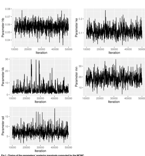
[37]), however, here we create a plot from the chains of the parameters’posterior marginals and check the chains visually (seeFig 1).
[image:10.612.77.574.176.710.2]plot_chains <- ga_plot_chains(data = mcmc_result$samples, from = 10000, steps = 50)
After cutting off the first 10,000 sample points, the chains show a reasonable mixing and no signs of burn-in or the adaptation phase of the algorithm. We have chosen the functionMCMC() from package adaptMCMC because it is largely self-tuning and therefore easy to use. An adapta-tion phase of 20,000 sample points seems to be sufficient in most cases. Nevertheless, it is impor-tant to keep in mind thatMCMC()calls a stochastic algorithm, which may fail to adapt, even for the data set we are using. If that happens, running the algorithm a second time usually suffices. If not, the adaptation phase might have to be enlarged and the chain might have to be run for a lon-ger time.
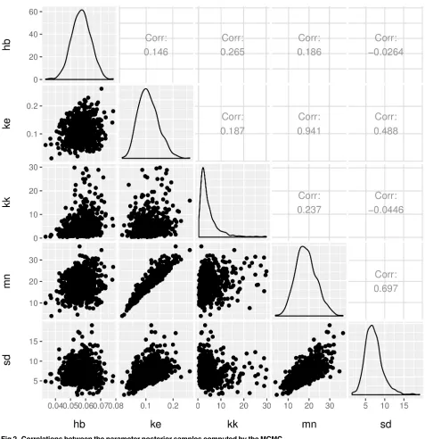
Next, we create a correlation plot, for the posterior parameter sample, computed by the MCMC. The parameters for our example co-vary as shown inFig 2.
The strongest correlation is observed between the threshold mean (mn) and the dominant rate constant (ke), which can be understood from eqs(1)and(2). Strong parameter correlations
could be viewed as indicators of over-parametrised models, however the equations of GUTS represent our understanding of the processes determining survival under stress. As such the model parameters have a mechanistic interpretation, which would be partially lost if reducing the model. Furthermore, reducing GUTS to fewer parameters would introduce additional strong assumptions and so GUTS would loose its generality. For example, disposing of the threshold parameter would imply the assumption that any infinitely small dose of the stressor will result in an increased hazard rate (see also [4]). An important insight fromFig 2is that sur-vival predictions must account for the correlation between parameters to properly account for parametric uncertainty.
Quantification of Parameter Uncertainty
To compute the uncertainty of each of the parameters, we calculate adequate quantiles from the posterior samples. Together with the maximum of the posterior distribution, these quan-tiles are then tabulated.
plot_corrs <- ga_plot_correlations(data = mcmc_result$samples, from = 10000, steps = 50)
tab_quant <- ga_tab_quantiles(data = mcmc_result$samples, log.p = mcmc_result$log.p, from = 10001)
print(tab_quant)
maxpost q0.025 q0.5 q0.975
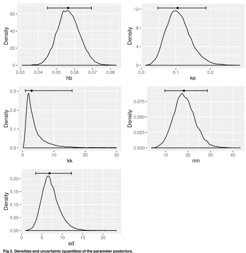
To inspect the distribution and the uncertainty visually, we plot the densities of each of the parameters.Fig 3shows the densities, and each plot contains a horizontal line indicating the uncertainty quantiles (the median is always added).
Fig 2. Correlations between the parameter posterior samples computed by the MCMC.
doi:10.1371/journal.pcbi.1004978.g002
Probabilistic Prediction and Validating the Model With New Data
[image:13.612.76.577.72.586.2]After calibrating our model with real data, we use it for probabilistic predictions. We demon-strate how to make probabilistic predictions (without survival data) and how to validate these predictions against measured survival data. In both cases we use fictional (“fake”) data, for demonstration purposes.
Fig 3. Densities and uncertainty (quantiles) of the parameter posteriors.
The data must contain concentrations and concentration time points, but also the time points at which we want to make predictions. Furthermore, we need to specify the initial num-ber of individuals (100, in our example). This numnum-ber is set in the first element of the vector of survivor counts (y). Unless we have validation data, the remaining values are not needed and set to an arbitrary value (0, in our example).
We tabulate the predictions and save the result in the R list objecttab_pred. We use the commandhead()to print the first 6 lines of the first table, however, all tables can be printed usingprint(tab_pred).
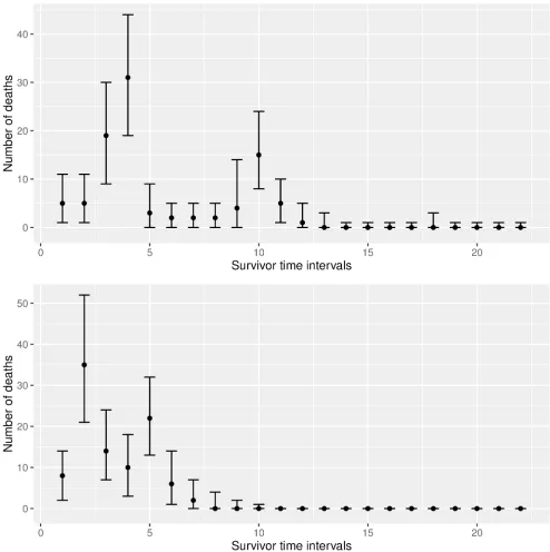
Finally, we create a prediction plot (seeFig 4). The plot shows the medians as well as the quantiles of the predicted survivor counts.
g_obj_new <- list(
guts_setup(C = c(99.97824, 0, 103.88, 0, 0, 103.56, 0, 0, 100.58, 96.51, 0, 2.35724),
Ct = c(0, 1.03, 3.01, 4.02, 8, 8.01, 15, 16, 16.01, 17, 18.01, 22.01),
y = c(100, rep(0, 22)), yt = 0:22),
guts_setup(C = c(101.343, 99.5066, 0, 98.19, 95.82, 0, 0, 0, 3.283),
Ct = c(0, 1.02, 2.99, 4.01, 9, 9.01, 11.01, 17.01, 22.01),
y = c(100, rep(0, 22)), yt = 0:22)
)
tab_pred <- ga_tab_predictions(gobjs = g_obj_new, data = mcmc_result$samples)
head(tab_pred[[1]])
ytd q0.025 q0.5 q0.975
1 1 2 5 11
2 2 2 5 10
3 3 9 19 30
4 4 19 31 44
5 5 0 3 8
6 6 0 2 5
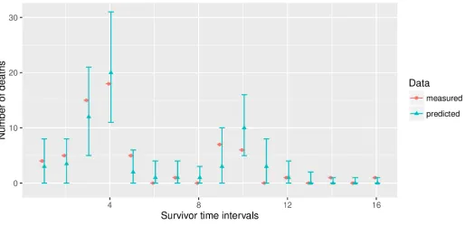
The prediction plots show the 95% probability bands and the medians, for the number of deaths that are predicted to occur in each observation window. If measured survivor data is present, it is also possible to add this information to the tables and plots, for validation. We modify our first fictional data set from above and add some (also fictional) survivor data. The tabulation now contains an additional column (“measured”), and the measured data (fictional data, in our example) is added to the plot as well (seeFig 5). Note that each single table can also be saved to text files using the commandwrite.csv().
Fig 4. Predictions for 2 fictional (“fake”) experimental setups.
Example Code and Further Development
The complete code used throughout the presentation here is available with the paper (seeS1 ScriptandS1 Data). We believe that the conciseness of our code and the application of our self-created wrapper functions make the procedures very easy to understand and to reproduce. However, with more expertise in R, users can easily alter our code and produce their own out-put. For instance, the plotting routines provided by the R package ggplot2 [38] are very power-ful and allow for rich-featured ready-to-publish graphics. We also encourage users to try out different optimisation and inference routines.
Future development will focus on the implementation of more distributions as well as fur-ther performance improvements. Users of our R package GUTS are encouraged to provide ideas, feedback or feature requests to the authors and the R GUTS user community, or to con-tribute actively to further development as a co-developer. The best way to communicate is via the mailing list of the package ([email protected]). The development home page of our R package GUTS can be found on R-Forge (https://r-forge.r-project.org/ projects/guts/).
g_obj_val <- guts_setup(C = c(99.97824, 0, 103.88, 0, 0, 103.56, 0, 0, 100.58, 96.51, 0, 2.35724),
Ct = c(0, 1.03, 3.01, 4.02, 8, 8.01, 15, 16, 16.01, 17, 18.01, 22.01),
y = c(66, 62, 57, 42, 24, 19, 19, 18, 18, 11, 5, 5, 4, 4, 3, 3, 2), yt = 0:16)
tab_val <- ga_tab_predictions(gobjs = list(g_obj_val), data = mcmc_result$samples, measured = TRUE)
print(tab_val[[1]])
ytd measured q0.025 q0.5 q0.975
1 1 4 1.000 4 8
2 2 5 0.975 3 8
3 3 15 5.000 12 21
4 4 18 12.000 20 30
5 5 5 0.000 2 6
6 6 0 0.000 1 4
7 7 1 0.000 1 4
8 8 0 0.000 1 4
9 9 7 0.000 3 10
10 10 6 4.000 10 17
11 11 0 0.000 3 8
12 12 1 0.000 1 4
13 13 0 0.000 0 2
14 14 1 0.000 0 1
15 15 0 0.000 0 1
16 16 1 0.000 0 1
Discussion and Future Directions
We discuss the modelling of survival under chemical stress using GUTS [4]. GUTS places the assumptions underlying survival modelling in a consistent mathematical framework, but the calibration has been a challenge. In particular the calibration of toxicodynamic parameters, and the estimation of parametric and predictive uncertainty was still a problem as it required much computational power and time.
GUTS is a survival analysis tool specifically designed to account for time-varying stressors. It is also possible to integrate multiple, independently acting stressors by adding hazard rates [25,26]. However, most intriguing are the possibilities to better understand underlying mecha-nisms my meaningful interpretation of the GUTS parameters. We expect that our software facilitates re-analyses of existing survival data as well as asking new research questions in a wide range of sciences. In particular the ability to quickly quantify stressor thresholds in con-junction with dynamic compensating processes, and their uncertainty, is an improvement that complements current survival analysis methods.
Supporting Information
S1 Script. GUTS example R script.Auxiliary R Script for the Paper“Computationally Effi-cient Implementation of a Novel Algorithm for the General Unified Threshold Model of Sur-vival (GUTS)”.
(R)
[image:17.612.64.578.76.326.2]S1 Data. GUTS example data.Example data for the Paper“Computationally Efficient Imple-mentation of a Novel Algorithm for the General Unified Threshold Model of Survival (GUTS)”. (TXT)
Fig 5. Comparison of a model forecast with fictional (“fake”) data.
Author Contributions
Conceived and designed the experiments: CA SV RA. Performed the experiments: CA SV RA. Analyzed the data: CA SV RA. Contributed reagents/materials/analysis tools: CA SV RA. Wrote the paper: CA SV RA. Developed the R package GUTS: CA SV.
References
1. Bliss C I. The method of probits. Science. 1934; 79(2037):38–39. doi:10.1126/science.79.2037.38
PMID:17813446
2. Newman M C, Unger M A. Fundamentals of Ecotoxicology. 2nd ed. Boca Raton: Lewis Publishers; 2003. isbn: 9781566705981
3. Chew R D, Hamilton M A. Toxicity curve estimation—fitting a compartment model to median survival times. Transactions of the American Fisheries Society. 1985; 114(3):403–412. doi:10.1577/1548-8659 (1985)114%3C403:TCE%3E2.0.CO;2
4. Jager T, Albert C, Preuss T G, Ashauer R. General Unified Threshold model of Survival—a toxicoki-netic toxicodynamic framework for ecotoxicology. Environmental Science & Technology. 2011; 45 (7):2529–2540. doi:10.1021/es103092a
5. Ceconi C, Ferrari R, Bachetti T, Opasich C, Volterrani M, Colombo B, et al. Chromogranin A in heart fail-ure: a novel neurohumoral factor and a predictor for mortality. European Heart Journal. 2002; 23 (12):967–974. doi:10.1053/euhj.2001.2977PMID:12069452
6. Selvin S. Survival analysis for epidemiologic and medical research: a practical guide. Cambridge: Cambridge University Press; 2008. isbn: 9780521895194
7. Mihaylova B, Emberson J, Blackwell L, Keech A, Simes J, Barnes E H, et al. The effects of lowering LDL cholesterol with statin therapy in people at low risk of vascular disease: Meta-analysis of individual data from 27 randomised trials. The Lancet. 2012; 380(9841):581–590. doi:10.1016/S0140-6736(12) 60367-5
8. Keiding N. Event history analysis and the cross-section. Statistics in Medicine. 2006; 25(14):2343– 2364. doi:10.1002/sim.2579PMID:16708345
9. Andersen P K, Keiding N. Multi-state models for event history analysis. Statistical Methods in Medical Research. 2002; 11(2):91–115. doi:10.1191/0962280202sm275edPMID:12040698
10. Balch C M, Soong S J, Gershenwald J E, Thompson J F, Reintgen D S, Cascinelli N, et al. Prognostic factors analysis of 17,600 melanoma patients: validation of the American Joint Committee on Cancer melanoma staging system. Journal of Clinical Oncology. 2001; 19(16):3622–3634. PMID:11504744 11. Garrett K A, Madden L V, Hughes G, Pfender W F. New applications of statistical tools in plant
pathol-ogy. Phytopatholpathol-ogy. 2004; 94(9):999–1003. doi:10.1094/PHYTO.2004.94.9.999PMID:18943077 12. Carnes B A, Holden L R, Olshansky S J, Witten M T, Siegel J S. Mortality partitions and their relevance
to research on senescence. Biogerontology. 2006; 7(4):183–198. doi:10.1007/s10522-006-9020-3
PMID:16732401
13. Gavrilov L A, Gavrilova N S. The reliability theory of aging and longevity. Journal of Theoretical Biology. 2001; 213(4):527–545. doi:10.1006/jtbi.2001.2430PMID:11742523
14. Lu H, Kolarik W J, Lu S S. Real-time performance reliability prediction. IEEE Transactions on Reliability. 2001; 50(4):353–357. doi:10.1109/24.983393
15. Au S K, Beck J L. Estimation of small failure probabilities in high dimensions by subset simulation. Prob-abilistic Engineering Mechanics. 2001; 16(4):263–277. doi:10.1016/S0266-8920(01)00019-4 16. Box-Steffensmeier J M, Reiter D, Zorn C. Nonproportional hazards and event history analysis in
inter-national relations. Journal of Conflict Resolution. 2003; 47(1):33–53. doi:10.1177/0022002702239510 17. Guo G. Event-history analysis for left-truncated data. Sociological Methodology. 1993; 23:217–243.
doi:10.2307/271011PMID:12318163
18. Nyman A-M, Schirmer K, Ashauer R. Toxicokinetic-toxicodynamic modelling of survival of Gammarus pulex in multiple pulse exposures to propiconazole: model assumptions, calibration data requirements and predictive power. Ecotoxicology. 2012; 21(7):1828–1840. doi:10.1007/s10646-012-0917-0PMID:
22562719
20. Jager T, Heugens E H W, Kooijman S A L M. Making sense of ecotoxicological test results: towards application of process-based models. Ecotoxicology. 2006; 15(3):305–314. doi: 10.1007/s10646-006-0060-xPMID:16739032
21. Ashauer R, Thorbek P, Warinton J S, Wheeler J R, Maund S. A method to predict and understand fish survival under dynamic chemical stress using standard ecotoxicity data. Environmental Toxicology and Chemistry. 2013; 23(4):954–965. doi:10.1002/etc.2144
22. Beaudouin R, Zeman F A, Péry A R R. Individual sensitivity distribution evaluation from survival data using a mechanistic model: implications for ecotoxicological risk assessment. Chemosphere. 2012; 89 (1):83–88. doi:10.1016/j.chemosphere.2012.04.021PMID:22572164
23. Kulkarni D, Daniels B, Preuss T G. Life-stage-dependent sensitivity of the cyclopoid copepod Mesocy-clops leuckarti to triphenyltin. Chemosphere. 2013; 92(9):1145–1153. doi:10.1016/j.chemosphere. 2013.01.076PMID:23466081
24. Gergs A, Jager T. Body size-mediated starvation resistance in an insect predator. Journal of Animal Ecology. 2014; 83(4):758–768. doi:10.1111/1365-2656.12195PMID:24417336
25. Nyman A-M, Hintermeister A, Schirmer K, Ashauer R. The insecticide Imidacloprid causes mortality of the freshwater amphipod Gammarus pulex by interfering with feeding behavior. PLoS ONE. 2013; 8(5): e62472. doi:10.1371/journal.pone.0062472PMID:23690941
26. Ashauer R, O’Connor I, Hintermeister A, Escher B. Death dilemma and organism recovery in ecotoxi-cology. Environmental Science & Technology. 2015; 49(16):10136–10146. doi:10.1021/acs.est. 5b03079
27. Albert C, Ashauer R, Künsch H R, Reichert P. Bayesian experimental design for a toxicokinetic-toxico-dynamic model. Journal of Statistical Planning and Inference. 2012; 142(1):263–275. doi:10.1016/j. jspi.2011.07.014
28. Andersen P K, Borgan O, Gill R D, Keiding N. Statistical Models Based on Counting Processes. New York: Springer; 1993. isbn: 9781461243489
29. Albert C, Vogel S. GUTS: fast calculation of the likelihood of a stochastic survival model. R Package Version 0.1. 2011 Jun 17
30. Albert C, Vogel S. GUTS: fast calculation of the likelihood of a stochastic survival model. R Package Version 1.0. 2015 Jun 26. Available from:http://CRAN.R-project.org/package=GUTS
31. R Core Team. R: a language and environment for statistical computing. Vienna: R Foundation for Sta-tistical Computing; 2015 Mar 9. Available from:http://www.r-project.org
32. Eddelbuettel D, Francois R. Rcpp: seamless R and C++ integration. Journal of Statistical Software. 2011; 40(8):1–18. doi:10.18637/jss.v040.i08
33. Eddelbuettel D. Seamless, R and C++ integration with Rcpp. New York: Springer; 2013. isbn: 978-1-4614-6867-7
34. Ashauer R, Hintermeister A, Caravatti I, Kretschmann A, Escher B I. Toxicokinetic and toxicodynamic modeling explains carry-over toxicity from exposure to diazinon by slow organism recovery. Environ-mental Science & Technology. 2010; 44(10):3963–3971. doi:10.1021/es903478b
35. Varadhan R, Johns Hopkins University, Borchers H W, ABB Corporate Research. dfoptim: derivative-free optimization. R package version 2011.8-1. 2011. Available from:http://CRAN.R-project.org/ package=dfoptim
36. Scheidegger A. adaptMCMC: implementation of a generic adaptive Monte Carlo Markov Chain sam-pler. R package version 1.1. 2012. Available from:http://CRAN.R-project.org/package=adaptMCMC 37. Plummer M, Best N, Cowles K, Vines K. CODA: convergence diagnosis and output analysis for MCMC.
R News. 2006; 6(1):7–11. Available from:http://CRAN.R-project.org/doc/Rnews/Rnews_2006-1.pdf 38. Wickham H. ggplot2: elegant graphics for data analysis. New York: Springer; 2009. isbn: