Comparison of exponential time series alignment and time series alignment using artificial neural networks by example of prediction of future development of stock prices of a specific company

Comparison of exponential time series

alignment and time series alignment using

artificial neural networks by example of

prediction of future development of stock prices

of a specific company

Jakub Horák1,Ύ_{, Tomáš Krulický}1

1_{Institute of Technology and Business in České Budějovice, School of Expertness and Valuation,}

Okružní 517/10, 370 01 České Budějovice, Czech Republic

Abstract. Accurate stock price prediction is very difficult in today's economy. Accurate prediction plays an important role in helping investors improve return on equity. As a result, a number of new approaches and technologies have logically evolved in recent years to predict stock prices. One is also the method of artificial neural networks, which have many advantages over conventional methods. The aim of this paper is to compare a method of exponential time series alignment and time series alignment using artificial neural networks as tools for predicting future stock price developments on the example of the company Unipetrol. Time series alignment is performed using artificial neural networks, exponential alignment of time series, and then a comparison of time series of predictions of future stock price trends predicted using the most successful neural network and price prediction calculated by exponential time series alignment is performed. Predictions for 62 business days were obtained. The realistic picture of further possible development is surprisingly given based on the exponential alignment of time series.

Key words: prediction, stock price, tome series, exponential alignment, artificial neural networks

1 Introduction

Time series are defined as sequences of spatially and de facto comparable observations which are organized based on time [1]. According to De Baets and Harvey [2], time series can be defined as ordered sequences of values of a variable at equidistant time intervals. According to the authors, time series analysis can be applied, for example, in process and quality control, in sales predictions, in census analysis, etc.

Currently, the application of time series is used in many different disciplines. Significant uses of time series include financial time or economic series that are very specific. Economic time series are often volatile, especially because over time, economic operators face different

circumstances that are constantly changing. Time series are routinely monitored at monthly, quarterly or annual intervals. However, the financial time series are monitored in the daily, sometimes hourly, timeframe [3].

One of the most important tasks of time series analysis is prediction. When predicting time series, it is considered a basic step to specify a given prediction problem. With prediction, you need to get the most accurate idea of the predictive variables, all available data and their nature, determine the prediction method, and set the prediction horizon. It is also important to decide whether data will be adjusted for the calculation, and if so, how. Because the prediction is needed for further decision making, it is best to know the system as much as possible [4].

Accurate stock price prediction is very difficult. Unpredictability is particularly noticeable as a result of the global financial crisis [5]. Accurate prediction of stock price movements plays a significant role in helping investors improve the return on their purchased stocks [6]. According to Vochozka [7], traditional stock price prediction methods can´t be analysed and applied well due to problems such as forecast inaccuracies, slow training rates, etc.

According to Ghiassi et al. [8], the analysis of stock price prediction includes many artificial intelligence approaches, especially artificial neural networks. According to Zhang (2004), a wide range of applications and new technologies have been developed over the last few years to predict stock prices such as the ARIMA method, artificial neural networks, etc. Artificial neural networks are currently considered a very effective method for analysing, collecting and predicting different data, so their use is possible in solving complex problems or in various complex situations [10].

It depends very much on the purpose of time series and on the nature of the data. As for the process of time series and neural networks, neural networks capture time series behavior and try to predict individual data points as best as they can. However, in order for neural networks to work best with the time series, it is very important to learn the neural networks correctly [11]. The efficiency of the proposed time series and learning process seems to be a good tool for predicting a very complex non-linear time series [12].

Artificial neural networks have many advantages over conventional methods. They are flexible in their own use, they can quickly and with high precision analyse complex patterns etc. [13]. According to Šuleř [14] their advantage lies in the accuracy of the results, the ability to work with large data, etc. According to Vochozka [15], the disadvantage of neural networks is their demand for large input data. To create such amount of data, many test observations are needed, which is demanding for users.

The ARIMA model is currently a widely used class of time series prediction models [16]. This model allows you to predict the behavior of time series in the future and understand their properties [17]. According to Mélard and Pasteels [18], the ARIMA model is mainly used for a short-term prognosis when data is not available or the model has poor prediction characteristics. We regard the prediction of future stock market values as one of the most needed financial applications. At present, the ARIMA model is often used to predict future stock price developments [19].

circumstances that are constantly changing. Time series are routinely monitored at monthly, quarterly or annual intervals. However, the financial time series are monitored in the daily, sometimes hourly, timeframe [3].

One of the most important tasks of time series analysis is prediction. When predicting time series, it is considered a basic step to specify a given prediction problem. With prediction, you need to get the most accurate idea of the predictive variables, all available data and their nature, determine the prediction method, and set the prediction horizon. It is also important to decide whether data will be adjusted for the calculation, and if so, how. Because the prediction is needed for further decision making, it is best to know the system as much as possible [4].

Accurate stock price prediction is very difficult. Unpredictability is particularly noticeable as a result of the global financial crisis [5]. Accurate prediction of stock price movements plays a significant role in helping investors improve the return on their purchased stocks [6]. According to Vochozka [7], traditional stock price prediction methods can´t be analysed and applied well due to problems such as forecast inaccuracies, slow training rates, etc.

According to Ghiassi et al. [8], the analysis of stock price prediction includes many artificial intelligence approaches, especially artificial neural networks. According to Zhang (2004), a wide range of applications and new technologies have been developed over the last few years to predict stock prices such as the ARIMA method, artificial neural networks, etc. Artificial neural networks are currently considered a very effective method for analysing, collecting and predicting different data, so their use is possible in solving complex problems or in various complex situations [10].

It depends very much on the purpose of time series and on the nature of the data. As for the process of time series and neural networks, neural networks capture time series behavior and try to predict individual data points as best as they can. However, in order for neural networks to work best with the time series, it is very important to learn the neural networks correctly [11]. The efficiency of the proposed time series and learning process seems to be a good tool for predicting a very complex non-linear time series [12].

Artificial neural networks have many advantages over conventional methods. They are flexible in their own use, they can quickly and with high precision analyse complex patterns etc. [13]. According to Šuleř [14] their advantage lies in the accuracy of the results, the ability to work with large data, etc. According to Vochozka [15], the disadvantage of neural networks is their demand for large input data. To create such amount of data, many test observations are needed, which is demanding for users.

The ARIMA model is currently a widely used class of time series prediction models [16]. This model allows you to predict the behavior of time series in the future and understand their properties [17]. According to Mélard and Pasteels [18], the ARIMA model is mainly used for a short-term prognosis when data is not available or the model has poor prediction characteristics. We regard the prediction of future stock market values as one of the most needed financial applications. At present, the ARIMA model is often used to predict future stock price developments [19].

Over the past twenty years, exponential alignment has been successful in many empirical studies, and is currently well established as an accurate prediction method. Exponential alignment is one of the many approaches to time series analysis. It is usually used to model a trendline component of time series (but can also be used for other time series components) that are not time-stable and are rapidly changing. If this is the case, normal decomposition can´t be used and other modelling methods such as ARIMA or other stochastic models [20] are sought. Applying exponential alignment to prognostic time series usually depends on three basic methods: simple exponential alignment, exponential alignment corrected by a trend and its seasonal variations. A common approach to selecting a method appropriate for

a specific time series is based on the validation of prediction on the retained portion of a sample using criteria such as a mean absolute percentage error [21].

The aim of the paper is to compare the method of exponential alignment of time series and time series alignment using artificial neural networks as tools for predicting future price development of the company on the example of Unipetrol.

2 Data and methods

Unipetrol is one of the most prominent business entities in the Czech Republic. Its activity, structure, vision and activity is characterized by the following [22]:

"Unipetrol is the most important refining and petrochemical group in the Czech Republic and one of the main players in Central Europe. In the Czech Republic, it is the largest oil processor, one of the most important plastic producers and the owner of the broadest petrol station network under the Benzina brand. Revenues in the group in 2016 amounted to 87.8 billion CZK. The Unipetrol Group has been part of the largest Central European refining and petrochemical group PKN Orlen, based in Poland, since 2005. The group is divided into two business segments: downstream (combining refinery and petro-chemistry) and retail fuel distribution. Within the downstream segment, the company operates refineries in Litvínov and Kralupy nad Vltavou. The group is number one on the Czech wholesale fuel market. In its Litvínov locality, the group operates an ethylene unit with subsequent polymer production. In 2016, Benzina's petrol station network with 363 petrol stations (as of 31 December 2016) and the estimated market share of 17.6% of the retail fuel sales was the leader in the Czech market (company estimate according to the Czech Statistical Office by October 2016). Within the subsidiaries PETROTRANS, s.r.o. and UNIPETROL DOPRAVA, s.r.o. the group operates a wide range of logistics and transportation services. Unipetrol R & D Center, a.s. in Ústí nad Labem and the Polymer Institute Brno branch are engaged in research and development in the field of petro-chemistry. As of 31 December 2016, the group employed more than 4,500 workers from various professions. The parent company of the group is UNIPETROL, a.s. "

Table 1. Data input statistics for the data file

Statistic Stock price (Output)

Minimum (Training) 105.5

Maximum (Training) 385

Average (Training) 198.86

Standard Deviation (Training) 64.58

Minimum (Testing) 107.5

Maximum (Testing) 380

Average (Testing) 195.96

Standard Deviation (Testing) 62.86

Minimum (Validation) 106

Maximum (Validation) 381

Average (Validation) 199.49

Standard deviation (Validation) 59.57

Minimum (Overall) 105.5

Maximum (Overall) 385

Average (Overall) 198.51

Standard Deviation (Overall) 64.49

Source: Authors.

2.1 Time series alignment using artificial neural networks

For data processing, DELL's Statistica version 12 will be used. The data mining tool of the neural network will be used. In particular, we will use time series (by regression).

We will generate Multilayer Perceptron Networks (MLP) and Neural Networks of Basic Radial Functions (RBF). Time will be the independent variable. We will determine the company's stock price as the dependent variable. We divide the time series into three sets - training, testing, and validation. The first group will be 70% of input data. Based on the training set of data, we generate neural structures. In the remaining two sets of data, we always leave 15% of the input information. Both groups will serve us to verify the reliability of the found neural structure or found model. The delay of the time series will be 1. We will generate 10,000 neural networks. Out of those we will preserve 5 with the best characteristics†_{. In the hidden layer, we will have at least two neurons, at most 20. In the case} of the radial core function, at least 21 neurons, at most 30, will be in the hidden layer. For the multilayer perceptron network, we will consider these activation functions in the hidden layer and in the output layer:

 Linear,  Logistic,  Atanh,  Exponential,  Sinus.

Other settings are left by default (ANS – automated neural network). The results, if the outputs are not adequate, can then be corrected by adjusting the weights of individual neurons in the structure using the VNS tool (own neural networks).

As soon as we generate neural networks, we will evaluate their validity on an expert basis, not just by statistical characteristics. Because of neural network shortcomings (black box,

† _{We will proceed using the smallest square method. We will terminate network generation if there is}

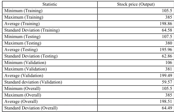
Table 1. Data input statistics for the data file

Statistic Stock price (Output)

Minimum (Training) 105.5

Maximum (Training) 385

Average (Training) 198.86

Standard Deviation (Training) 64.58

Minimum (Testing) 107.5

Maximum (Testing) 380

Average (Testing) 195.96

Standard Deviation (Testing) 62.86

Minimum (Validation) 106

Maximum (Validation) 381

Average (Validation) 199.49

Standard deviation (Validation) 59.57

Minimum (Overall) 105.5

Maximum (Overall) 385

Average (Overall) 198.51

Standard Deviation (Overall) 64.49

Source: Authors.

2.1 Time series alignment using artificial neural networks

For data processing, DELL's Statistica version 12 will be used. The data mining tool of the neural network will be used. In particular, we will use time series (by regression).

We will generate Multilayer Perceptron Networks (MLP) and Neural Networks of Basic Radial Functions (RBF). Time will be the independent variable. We will determine the company's stock price as the dependent variable. We divide the time series into three sets - training, testing, and validation. The first group will be 70% of input data. Based on the training set of data, we generate neural structures. In the remaining two sets of data, we always leave 15% of the input information. Both groups will serve us to verify the reliability of the found neural structure or found model. The delay of the time series will be 1. We will generate 10,000 neural networks. Out of those we will preserve 5 with the best characteristics†_{. In the hidden layer, we will have at least two neurons, at most 20. In the case} of the radial core function, at least 21 neurons, at most 30, will be in the hidden layer. For the multilayer perceptron network, we will consider these activation functions in the hidden layer and in the output layer:

 Linear,  Logistic,  Atanh,  Exponential,  Sinus.

Other settings are left by default (ANS – automated neural network). The results, if the outputs are not adequate, can then be corrected by adjusting the weights of individual neurons in the structure using the VNS tool (own neural networks).

As soon as we generate neural networks, we will evaluate their validity on an expert basis, not just by statistical characteristics. Because of neural network shortcomings (black box,

† _{We will proceed using the smallest square method. We will terminate network generation if there is}

no improvement, ie the reduction of the sum of squares value. Thus, we will preserve those neural structures whose sum of squares of residues to actual gold development will be as low as possible (ideally zero).

neural network overflow, etc.), neural networks may have excellent statistical parameters but won't be usable for realistic predictions. We will confront the predictions of the most successful networks between each other. Price developments will be predicted for the next 62 days on which the stocks will be traded. However, it should be noted that the prediction of the course of the price development is likely to be inaccurate. We will expect greater precision when predicting the price for the next one day after the input data set.

2.2 Exponential alignment of time series

DELL's Statistica software will also be used for processing. Specifically, it will be a module of advanced models. In them, we select time series / prediction. We then choose Exponential alignment and Prediction. The analysis settings will be as follows:-

1. We will use the model with exponential, 2. A seasonal component will not be established, 3. Alpha and Gamma will be both set to 0.1, 4. We will predict for the next 62 business days, 5. Set the maximum number of iterations to 50, 6. The convergence criterium will be 0.0001,

7. The compliance rate indicator will be the mean average square of the error, 8. Keep the other settings as default.

2.3 Comparison of time series

Finally, we compare the time series, i.e. the prediction of future stock price developments predicted by the most successful neural network and the prediction of prices calculated by exponential time series alignment.

3 Results

3.1 Time series alignment using artificial neural networks

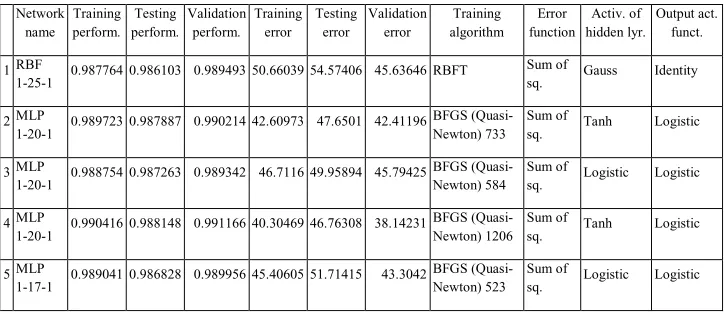
Table 2 provides 5 neural networks with the best characteristics out of 10,000 generated structures.

Table 2. Overview of preserved neural networks

Network name Training perform. Testing perform. Validation perform. Training error Testing error Validation error Training algorithm Error function Activ. of hidden lyr. Output act. funct.

1 RBF

1-25-1 0.987764 0.986103 0.989493 50.66039 54.57406 45.63646 RBFT

Sum of

sq. Gauss Identity

2 MLP

1-20-1 0.989723 0.987887 0.990214 42.60973 47.6501 42.41196 BFGS (Quasi-Newton) 733 Sum of

sq. Tanh Logistic

3 MLP

1-20-1 0.988754 0.987263 0.989342 46.7116 49.95894 45.79425 BFGS (Quasi-Newton) 584 Sum of

sq. Logistic Logistic

4 MLP

1-20-1 0.990416 0.988148 0.991166 40.30469 46.76308 38.14231 BFGS (Quasi-Newton) 1206 Sum of

sq. Tanh Logistic

5 MLP

1-17-1 0.989041 0.986828 0.989956 45.40605 51.71415 43.3042 BFGS (Quasi-Newton) 523 Sum of

sq. Logistic Logistic

The first neural network differs from others. It is a neural network of the basic radial function. The RBFT was used as a training algorithm. As with other preserved neural networks, the error function was determined by the sum of the smallest squares. For the activation of neurons in a hidden layer, Gauss function is used, for the activation of the output layer of neurons, identity is used. Other preserved neural networks are multilayer perceptron neural networks (MLPs). All were created using the Quasi-Newton algorithm (always using a different version). To activate the hidden layer of neurons, they use two functions – namely hyperbolic tangent and logistic functions. To activate neurons the outer layer uses a single function – logistic. The performance of the neural network is described by the value of the correlation coefficient. Correlation coefficients of all preserved networks and all data sets are shown in Table 3.

Table 3. Performance of preserved neural networks

Neural network Training perform. Testing perform. Validation perform. RBF 1-25-1 0.987764 0.986103 0.989493 MLP 1-20-1 0.989723 0.987887 0.990214 MLP 1-20-1 0.988754 0.987263 0.989342 MLP 1-20-1 0.990416 0.988148 0.991166 MLP 1-17-1 0.989041 0.986828 0.989956

Source: Authors.

We are ideally searching for such a neural network, which has a correlation coefficient ideally the closest to 1. The performance of all three sets should be ideally similar. This means that the structure created by the training set of data is valid and validated on the other two data sets. Of course, we must not forget that the neural network should have minimal errors in all three sets of data. The value of the correlation coefficients of all neuronal structures and data sets is always higher than 0.986. Differences between individual neural networks are minimal. This will be important in analysis of prediction statistics (see Table 4 below).

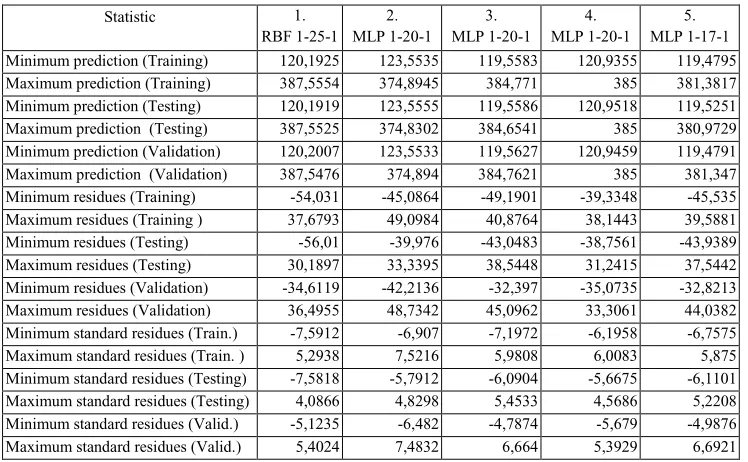
Table 4. Prediction statistics of individual neural structures

Statistic 1. RBF 1-25-1

2. MLP 1-20-1

3. MLP 1-20-1

4. MLP 1-20-1

5. MLP 1-17-1 Minimum prediction (Training) 120,1925 123,5535 119,5583 120,9355 119,4795 Maximum prediction (Training) 387,5554 374,8945 384,771 385 381,3817 Minimum prediction (Testing) 120,1919 123,5555 119,5586 120,9518 119,5251 Maximum prediction (Testing) 387,5525 374,8302 384,6541 385 380,9729 Minimum prediction (Validation) 120,2007 123,5533 119,5627 120,9459 119,4791 Maximum prediction (Validation) 387,5476 374,894 384,7621 385 381,347 Minimum residues (Training) -54,031 -45,0864 -49,1901 -39,3348 -45,535 Maximum residues (Training ) 37,6793 49,0984 40,8764 38,1443 39,5881 Minimum residues (Testing) -56,01 -39,976 -43,0483 -38,7561 -43,9389 Maximum residues (Testing) 30,1897 33,3395 38,5448 31,2415 37,5442 Minimum residues (Validation) -34,6119 -42,2136 -32,397 -35,0735 -32,8213 Maximum residues (Validation) 36,4955 48,7342 45,0962 33,3061 44,0382 Minimum standard residues (Train.) -7,5912 -6,907 -7,1972 -6,1958 -6,7575 Maximum standard residues (Train. ) 5,2938 7,5216 5,9808 6,0083 5,875 Minimum standard residues (Testing) -7,5818 -5,7912 -6,0904 -5,6675 -6,1101 Maximum standard residues (Testing) 4,0866 4,8298 5,4533 4,5686 5,2208 Minimum standard residues (Valid.) -5,1235 -6,482 -4,7874 -5,679 -4,9876 Maximum standard residues (Valid.) 5,4024 7,4832 6,664 5,3929 6,6921

The first neural network differs from others. It is a neural network of the basic radial function. The RBFT was used as a training algorithm. As with other preserved neural networks, the error function was determined by the sum of the smallest squares. For the activation of neurons in a hidden layer, Gauss function is used, for the activation of the output layer of neurons, identity is used. Other preserved neural networks are multilayer perceptron neural networks (MLPs). All were created using the Quasi-Newton algorithm (always using a different version). To activate the hidden layer of neurons, they use two functions – namely hyperbolic tangent and logistic functions. To activate neurons the outer layer uses a single function – logistic. The performance of the neural network is described by the value of the correlation coefficient. Correlation coefficients of all preserved networks and all data sets are shown in Table 3.

Table 3. Performance of preserved neural networks

Neural network Training perform. Testing perform. Validation perform. RBF 1-25-1 0.987764 0.986103 0.989493 MLP 1-20-1 0.989723 0.987887 0.990214 MLP 1-20-1 0.988754 0.987263 0.989342 MLP 1-20-1 0.990416 0.988148 0.991166 MLP 1-17-1 0.989041 0.986828 0.989956

Source: Authors.

We are ideally searching for such a neural network, which has a correlation coefficient ideally the closest to 1. The performance of all three sets should be ideally similar. This means that the structure created by the training set of data is valid and validated on the other two data sets. Of course, we must not forget that the neural network should have minimal errors in all three sets of data. The value of the correlation coefficients of all neuronal structures and data sets is always higher than 0.986. Differences between individual neural networks are minimal. This will be important in analysis of prediction statistics (see Table 4 below).

Table 4. Prediction statistics of individual neural structures

Statistic 1. RBF 1-25-1

2. MLP 1-20-1

3. MLP 1-20-1

4. MLP 1-20-1

5. MLP 1-17-1 Minimum prediction (Training) 120,1925 123,5535 119,5583 120,9355 119,4795 Maximum prediction (Training) 387,5554 374,8945 384,771 385 381,3817 Minimum prediction (Testing) 120,1919 123,5555 119,5586 120,9518 119,5251 Maximum prediction (Testing) 387,5525 374,8302 384,6541 385 380,9729 Minimum prediction (Validation) 120,2007 123,5533 119,5627 120,9459 119,4791 Maximum prediction (Validation) 387,5476 374,894 384,7621 385 381,347 Minimum residues (Training) -54,031 -45,0864 -49,1901 -39,3348 -45,535 Maximum residues (Training ) 37,6793 49,0984 40,8764 38,1443 39,5881 Minimum residues (Testing) -56,01 -39,976 -43,0483 -38,7561 -43,9389 Maximum residues (Testing) 30,1897 33,3395 38,5448 31,2415 37,5442 Minimum residues (Validation) -34,6119 -42,2136 -32,397 -35,0735 -32,8213 Maximum residues (Validation) 36,4955 48,7342 45,0962 33,3061 44,0382 Minimum standard residues (Train.) -7,5912 -6,907 -7,1972 -6,1958 -6,7575 Maximum standard residues (Train. ) 5,2938 7,5216 5,9808 6,0083 5,875 Minimum standard residues (Testing) -7,5818 -5,7912 -6,0904 -5,6675 -6,1101 Maximum standard residues (Testing) 4,0866 4,8298 5,4533 4,5686 5,2208 Minimum standard residues (Valid.) -5,1235 -6,482 -4,7874 -5,679 -4,9876 Maximum standard residues (Valid.) 5,4024 7,4832 6,664 5,3929 6,6921

Source: Authors.

If we monitor the statistics of the predictions of individual neural networks, we necessarily conclude that the differences between the networks are absolutely minimal for all statistics.

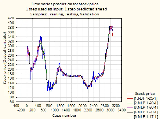
The graphical development of prices and predictions can also tell us the right outcome. Figure 1 provides a graphical comparison of Unipetrol's actual stock prices and predictions calculated using all neural networks.

Source: Authors.

It can be seen from the picture that all networks have more or less accurately copied the real price movements in past data. However, at some moments, for example on the 100th trading day, the stock price fluctuated downwards. These fluctuations, but in both directions, are repeated several times. It is a question of how far they are the result of a turbulent environment that none of the preserved neural networks has been able to reliably describe. However, despite this fact, we can assume that all preserved neural networks are applicable in practice.

Source: Authors.

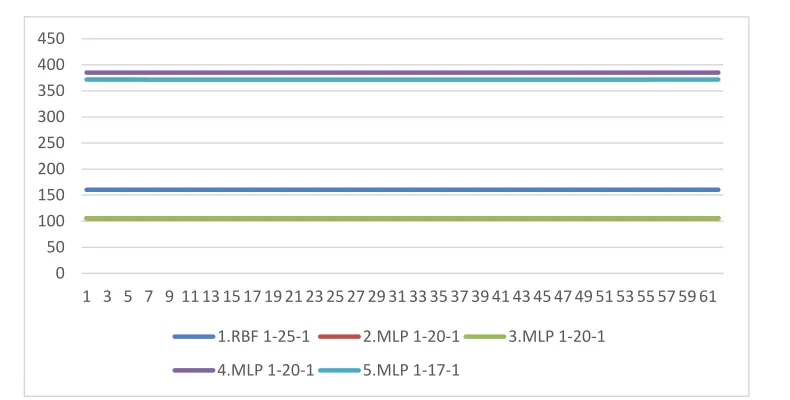
It is clear from the graph that networks are always (or almost always) predicting a constant development of Unipetrol's stock price over the review period. The only network that does not predict the constant development of stock prices over the projection period is Network Number 5, MLP 1-17-1. However, the price differences between days vary at the level of one thousand CZK. There is a significant difference between the predictions of individual networks. At first glance, and in view of price trends so far, the constant price seems unlikely to be in the observed period of 62 days.

Table 5 provides a detailed view of selected prediction cases. Specifically, this is about every tenth case of prediction.

Table 5. Values of selected predictions by individual neural networks

Case 1.RBF 1-25-1

2.MLP 1-20-1

3.MLP 1-20-1

4.MLP 1-20-1

5.MLP

1-17-1 Maximum Minimum Difference max – min

% of max. price 10 160.364 105.5 105.5 385 371.766 385 105.5 279.5 72.60 % 20 160.364 105.5 105.5 385 371.7664 385 105.5 279.5 72.60 % 30 160.364 105.5 105.5 385 371.7667 385 105.5 279.5 72.60 % 40 160.364 105.5 105.5 385 371.767 385 105.5 279.5 72.60 % 50 160.364 105.5 105.5 385 371.7673 385 105.5 279.5 72.60 % 60 160.364 105.5 105.5 385 371.7676 385 105.5 279.5 72.60 %

Source: Authors.

The table shows that the 2nd and 3rd neural networks have exactly the same predictions. This is always the minimum amount of predictions at a given time. Other predictions are higher. The table below also offers a summary of the maximum and minimum predictions of the case. It also calculates the difference between the minimum and maximum predictions. Subsequently, this difference is compared to the maximum predicted and expressed as a percentage of the difference to the maximum prediction. We find that the difference between the minimum and maximum predictions is 72.6%. Therefore, it is clear that the interval between the lowest and the highest predictions is too large for the future estimate. This means that the actual price may move at this interval, but the value of the prediction is zero for the

Ϭ ϱϬ ϭϬϬ ϭϱϬ ϮϬϬ ϮϱϬ ϯϬϬ ϯϱϬ ϰϬϬ ϰϱϬ

ϭ ϯ ϱ ϳ ϵ ϭϭ ϭϯ ϭϱ ϭϳ ϭϵ Ϯϭ Ϯϯ Ϯϱ Ϯϳ Ϯϵ ϯϭ ϯϯ ϯϱ ϯϳ ϯϵ ϰϭ ϰϯ ϰϱ ϰϳ ϰϵ ϱϭ ϱϯ ϱϱ ϱϳ ϱϵ ϲϭ

ϭ͘Z&ϭͲϮϱͲϭ Ϯ͘D>WϭͲϮϬͲϭ ϯ͘D>WϭͲϮϬͲϭ

Source: Authors.

It is clear from the graph that networks are always (or almost always) predicting a constant development of Unipetrol's stock price over the review period. The only network that does not predict the constant development of stock prices over the projection period is Network Number 5, MLP 1-17-1. However, the price differences between days vary at the level of one thousand CZK. There is a significant difference between the predictions of individual networks. At first glance, and in view of price trends so far, the constant price seems unlikely to be in the observed period of 62 days.

Table 5 provides a detailed view of selected prediction cases. Specifically, this is about every tenth case of prediction.

Table 5. Values of selected predictions by individual neural networks

Case 1.RBF 1-25-1

2.MLP 1-20-1

3.MLP 1-20-1

4.MLP 1-20-1

5.MLP

1-17-1 Maximum Minimum Difference max – min

% of max. price 10 160.364 105.5 105.5 385 371.766 385 105.5 279.5 72.60 % 20 160.364 105.5 105.5 385 371.7664 385 105.5 279.5 72.60 % 30 160.364 105.5 105.5 385 371.7667 385 105.5 279.5 72.60 % 40 160.364 105.5 105.5 385 371.767 385 105.5 279.5 72.60 % 50 160.364 105.5 105.5 385 371.7673 385 105.5 279.5 72.60 % 60 160.364 105.5 105.5 385 371.7676 385 105.5 279.5 72.60 %

Source: Authors.

The table shows that the 2nd and 3rd neural networks have exactly the same predictions. This is always the minimum amount of predictions at a given time. Other predictions are higher. The table below also offers a summary of the maximum and minimum predictions of the case. It also calculates the difference between the minimum and maximum predictions. Subsequently, this difference is compared to the maximum predicted and expressed as a percentage of the difference to the maximum prediction. We find that the difference between the minimum and maximum predictions is 72.6%. Therefore, it is clear that the interval between the lowest and the highest predictions is too large for the future estimate. This means that the actual price may move at this interval, but the value of the prediction is zero for the

Ϭ ϱϬ ϭϬϬ ϭϱϬ ϮϬϬ ϮϱϬ ϯϬϬ ϯϱϬ ϰϬϬ ϰϱϬ

ϭ ϯ ϱ ϳ ϵ ϭϭ ϭϯ ϭϱ ϭϳ ϭϵ Ϯϭ Ϯϯ Ϯϱ Ϯϳ Ϯϵ ϯϭ ϯϯ ϯϱ ϯϳ ϯϵ ϰϭ ϰϯ ϰϱ ϰϳ ϰϵ ϱϭ ϱϯ ϱϱ ϱϳ ϱϵ ϲϭ

ϭ͘Z&ϭͲϮϱͲϭ Ϯ͘D>WϭͲϮϬͲϭ ϯ͘D>WϭͲϮϬͲϭ

ϰ͘D>WϭͲϮϬͲϭ ϱ͘D>WϭͲϭϳͲϭ

investor. However, if we expertly assess predictions for the next day, we would choose the network number 5, i.e. MLP 1-17-1 as the most successful. On the imaginary second place, we would put network number 4, MLP 1-20-1.

3.2 Exponential alignment of time series

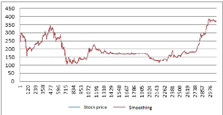
Figure 3 shows a comparison of the actual time series (blue curve) and the aligned time series (orange curve).

Source: Authors.

Source: Authors.

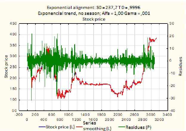
In essence, this is a graph that matches the figure 3. However, this is a box graph that provides the second variable for comparison. In addition, residues of an exponentially aligned time curve are displayed. The colour of the exponentially aligned curve, which is now red, has changed as opposed to the graph in figure 3. We can now follow the curve of residues, which are presented in green colour. The x-axis for the residue graph is on the right side of the image. The residual value ranges from -32 to 22 CZK per stock. In relative terms, we range from approximately - 15% to the average stock price to 10%. Because these are extreme values, we can boldly state that the model appears at first glance as very interesting.

3.3 Comparison of methods

Source: Authors.

In essence, this is a graph that matches the figure 3. However, this is a box graph that provides the second variable for comparison. In addition, residues of an exponentially aligned time curve are displayed. The colour of the exponentially aligned curve, which is now red, has changed as opposed to the graph in figure 3. We can now follow the curve of residues, which are presented in green colour. The x-axis for the residue graph is on the right side of the image. The residual value ranges from -32 to 22 CZK per stock. In relative terms, we range from approximately - 15% to the average stock price to 10%. Because these are extreme values, we can boldly state that the model appears at first glance as very interesting.

3.3 Comparison of methods

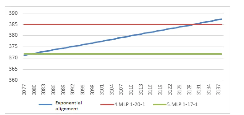
In order to better compare the use of both methods, i.e. artificial neural networks and exponential time series alignment, we will also use the graph (see Figure 5).

Source: Authors.

For comparison, we used the neural network number 4 and 5, in particular MLP 1-20-1 and MLP 1-17-1, in addition to prediction using exponential time series alignment. Both neural networks predict constant or near-price development. However, this may seem unlikely, as we predict the price for 62 business days (i.e. for more than 2 months). Looking at Unipetrol's stock price so far, we find that there is no analogy in the past where the price of stocks remains constant. Logically, the development predicted by the exponential alignment of time series appears more suitable. Over 62 business days, the company's stock price is expected to grow from approximately 371 CZK to 387 CZK. The change in the 16 CZK is realistic (in relative terms it is a change of less than 3.7% of the price).

4 Conclusion

The aim of the paper was to compare the method of exponential alignment of time series and time series alignment using artificial neural networks as tools for predicting future price development of a company, as exemplified on Unipetrol.

First, the data file was analysed. Subsequently, neural networks were generated, of which five with the best characteristics were preserved. Using statistically interpreted results, it has been found that it is possible to use up to two neural networks in practice: 4 (MLP 1-20-1) and 5 (MLP 1-17-1).

Then, the exponential alignment of time series was used. A prediction was obtained for 62 business days, which was then compared to the results of two preserved neural networks. At the time of the calculations it was not possible to determine which prediction is or is not correct. Based on a simple argumentation, we have inclined to the fact that, a realistic picture of further development is given rather by a prediction based on an exponential alignment of time series.

tools such as ARIMA. We will find further developments in the stock prices and verify their interpretation with subsequent real stock price developments.

References

1. M. Sheikhan, N. Mohammadi, Time series prediction using PSO-optimized neural network and hybrid feature selection algorithm for IEEE load data: revue littéraire mensuelle. Neural Computing and Applications, 23(3-4), 1185-1194, (2013)

2. S. De Baets, N. Harvey, Forecasting from time series subject to sporadic perturbations: Effectiveness of different types of forecasting support. International Journal of Forecasting, 34(2), 163-180, (2018)

3. J. Jaramillo, J. D. Velasquez, C. J. Franco, Research in Financial Time Series Forecasting with SVM: Contributions from Literature. IEEE Latin America Transactions, 15(1), 145-153, (2017)

4. P. Rostan, A. Rostan, The versatility of spectrum analysis for forecasting financial time series. Journal of Forecasting, 37(3), 327-339, (2018)

5. S. Hašková, Prediction of Future Development of Share Prices Using Neural Networks Based on Daily and Monthly Share Price Data. Mladá veda, 5(9), 33-48, (2017) 6. Z. Qun, L. Xu, G. Zhang, LSTM Neural Network with Emotional Analysis for

Prediction of Stock Price. Engineering Letters, 25(2), 167-175, (2017)

7. M. Vochozka, Inventory management using artificial neural networks in a concrete case. Proceedings of the 5th _{International Conference Innovation Management,} Entrepreneurship and Sustainability, Prague, Czech Republic, 1084-1094, (2017) 8. M. Ghiassi, H. Saidane, D. K. Zimbra, A dynamic artificial neural network model for

forecasting time series events. International Journal of Forecasting, 21(2), 341-362, (2005)

9. X. Zhang, Evolution of ARMA demand in supply chains. Manufacturing and Service Operations Management, 6(2), 195-198, (2004)

10. J. Vrbka, Z. Rowland, Stock price development forecasting using neural networks. Proceedings of the International conference Innovative Economic Symposium 2017, Strategic Partnerships in International Trade, Web of Conferences, 39, (2017)

11. Y. H. Hu, J. Hwang, Handbook of neural network signal processing. Boca Raton: CRC Press, (2002)

12. Y. Chen, B. Yang, J. Dong, Time-series prediction using a local linear wavelet neural network. Neurocomputing, 69(4-6), 449-465, (2006)

13. D. Santin, On the approximation of production functions: a comparison of artificial neural networks frontiers and efficiency techniques. Applied Economics Letters, 15(8), 597-600, (2008)

14. P. Šuleř, Using Kohonen´s neural networks to identify the bankruptcy of enterprises: Case study based on construction companies in South Bohemian region. Proceedings of the 5th _{International Conference Innovation Management, Entrepreneurship and} Sustainability, Prague, Czech Republic, 985-995, (2017)

15. M. Vochozka, Formation of complex company evaluation method through neural networks based on the example of construction companies collection. AD ALTA: Journal of Interdisciplinary Research, 7(2), 232-239, (2018)

tools such as ARIMA. We will find further developments in the stock prices and verify their interpretation with subsequent real stock price developments.

References

1. M. Sheikhan, N. Mohammadi, Time series prediction using PSO-optimized neural network and hybrid feature selection algorithm for IEEE load data: revue littéraire mensuelle. Neural Computing and Applications, 23(3-4), 1185-1194, (2013)

2. S. De Baets, N. Harvey, Forecasting from time series subject to sporadic perturbations: Effectiveness of different types of forecasting support. International Journal of Forecasting, 34(2), 163-180, (2018)

3. J. Jaramillo, J. D. Velasquez, C. J. Franco, Research in Financial Time Series Forecasting with SVM: Contributions from Literature. IEEE Latin America Transactions, 15(1), 145-153, (2017)

4. P. Rostan, A. Rostan, The versatility of spectrum analysis for forecasting financial time series. Journal of Forecasting, 37(3), 327-339, (2018)

5. S. Hašková, Prediction of Future Development of Share Prices Using Neural Networks Based on Daily and Monthly Share Price Data. Mladá veda, 5(9), 33-48, (2017) 6. Z. Qun, L. Xu, G. Zhang, LSTM Neural Network with Emotional Analysis for

Prediction of Stock Price. Engineering Letters, 25(2), 167-175, (2017)

7. M. Vochozka, Inventory management using artificial neural networks in a concrete case. Proceedings of the 5th _{International Conference Innovation Management,} Entrepreneurship and Sustainability, Prague, Czech Republic, 1084-1094, (2017) 8. M. Ghiassi, H. Saidane, D. K. Zimbra, A dynamic artificial neural network model for

forecasting time series events. International Journal of Forecasting, 21(2), 341-362, (2005)

9. X. Zhang, Evolution of ARMA demand in supply chains. Manufacturing and Service Operations Management, 6(2), 195-198, (2004)

10. J. Vrbka, Z. Rowland, Stock price development forecasting using neural networks. Proceedings of the International conference Innovative Economic Symposium 2017, Strategic Partnerships in International Trade, Web of Conferences, 39, (2017)

11. Y. H. Hu, J. Hwang, Handbook of neural network signal processing. Boca Raton: CRC Press, (2002)

12. Y. Chen, B. Yang, J. Dong, Time-series prediction using a local linear wavelet neural network. Neurocomputing, 69(4-6), 449-465, (2006)

13. D. Santin, On the approximation of production functions: a comparison of artificial neural networks frontiers and efficiency techniques. Applied Economics Letters, 15(8), 597-600, (2008)

14. P. Šuleř, Using Kohonen´s neural networks to identify the bankruptcy of enterprises: Case study based on construction companies in South Bohemian region. Proceedings of the 5th _{International Conference Innovation Management, Entrepreneurship and} Sustainability, Prague, Czech Republic, 985-995, (2017)

15. M. Vochozka, Formation of complex company evaluation method through neural networks based on the example of construction companies collection. AD ALTA: Journal of Interdisciplinary Research, 7(2), 232-239, (2018)

16. P. H. B. F. Franses, The Econometric Modelling of Financial Time Series. International Journal of Forecasting, 16(3), 426-427, (2000)

17. A. B. Sánchez, C. Ordóñez, F. S. Lasheras, F. J. De Cos Juez, J. Roca-Pardiñas, Forecasting SO 2 Pollution Incidents by means of Elman Artificial Neural Networks and ARIMA Models. Abstract and Applied Analysis, 1-6, (2013)

18. G. Mélard, J. M. Pasteels, Automatic ARIMA modeling including interventions, using time series expert software. International Journal of Forecasting, 16(4), 497-508, (2000)

19. M. F. Anaghi, Y. Norouzi, A Model for Stock Price Forecasting Based on ARMA Systems. 2nd _{International Conference on Advances in Computational Tools for} Engineering Applications, Beirut, Lebanon, 265-268, (2012)

20. L. Marek, M. Vrabec, ARIMA models and exponential smoothing. 33rd International Conference on Mathematical Methods in Economics, Czech Republic, 502-507, (2015) 21. B. Billah, M. L. King, R. D. Snyder, A. B. Koehler, Exponential smoothing model

selection for forecasting. International Journal of Forecasting, 22(2), 239-247, (2006) 22. Unipetrol, Unipetrol company in brief [online], Available at: