Parallel & Distributed Simulation Systems/Richard Fujimoto
Surviving the Design of Microprocessor and Multimicroprocessor Systems: Lessons Learned/Veljko Milutinovic
Mobile Processing in Distributed and Open Environments/Peter Sapaty
Introduction to Parallel Algorithms/C. Xavier and S.S. Iyengar
Solutions to Parallel and Distributed Computing Problems: Lessons from Biological Sciences/Albert Y. Zomaya, Fikret Ercal, and Stephan Olariu (Editors)
New Parallel Algorithms for Direct Solution of Linear Equations/
C. Siva Ram Murthy, K.N. Balasubramanya Murthy, and Srinivas Aluru
Practical PRAM Programming/Joerg Keller, Christoph Kessler, and Jesper Larsson Traeff
Computational Collective Intelligence/Tadeusz M. Szuba
Parallel & Distributed Computing: A Survey of Models, Paradigms, and Approaches/Claudia Leopold
Fundamentals of Distributed Object Systems: A CORBA Perspective/Zahir Tari and Omran Bukhres
Pipelined Processor Farms: Structured Design for Embedded Parallel Systems/Martin Fleury and Andrew Downton
Handbook of Wireless Networks and Mobile Computing/Ivan Stojmenoviic (Editor)
Internet-Based Workflow Management: Toward a Semantic Web/
Dan C. Marinescu
Parallel Computing on Heterogeneous Networks/Alexey L. Lastovetsky
Tools and Environments for Parallel and Distributed Computing Tools/
Salim Hariri and Manish Parashar
Distributed Computing: Fundamentals, Simulations and Advanced Topics, Second Edition/Hagit Attiya and Jennifer Welch
Smart Environments: Technology, Protocols and Applications/
Diane J. Cook and Sajal K. Das (Editors)
Fundamentals of Computer Organization and Architecture/Mostafa Abd-El-Barr and Hesham El-Rewini
ADVANCED COMPUTER
ARCHITECTURE AND
PARALLEL PROCESSING
Hesham El-Rewini
Southern Methodist UniversityMostafa Abd-El-Barr
Kuwait UniversityCopyright#2005 by John Wiley & Sons, Inc. All rights reserved.
Published by John Wiley & Sons, Inc., Hoboken, New Jersey. Published simultaneously in Canada.
No part of this publication may be reproduced, stored in a retrieval system, or transmitted in any form or by any means, electronic, mechanical, photocopying, recording, scanning, or otherwise, except as permitted under Section 107 or 108 of the 1976 United States Copyright Act, without either the prior written permission of the Publisher, or authorization through payment of the appropriate per-copy fee to the Copyright Clearance Center, Inc., 222 Rosewood Drive, Danvers, MA 01923,
for permission should be addressed to the Permissions Department, John Wiley & Sons, Inc., 111 River Street, Hoboken, NJ 07030, (201) 748-6011, fax (201) 748-6008.
Limit of Liability/Disclaimer of Warranty: While the publisher and author have used their best efforts in preparing this book, they make no representations or warranties with respect to the accuracy or completeness of the contents of this book and specifically disclaim any implied warranties of merchantability or fitness for a particular purpose. No warranty may be created or extended by sales representatives or written sales materials. The advice and strategies contained herein may not be suitable for your situation. You should consult with a professional where appropriate. Neither the publisher nor author shall be liable for any loss of profit or any other commercial damages, including but not limited to special, incidental, consequential, or other damages.
For general information on our other products and services please contact our Customer Care Department within the U.S. at 877-762-2974, outside the U.S. at 317-572-3993 or fax 317-572-4002.
Wiley also publishes its books in a variety of electronic formats. Some content that appears in print, however, may not be available in electronic format.
Library of Congress Cataloging-in-Publication Data is available
ISBN 0-471-46740-5
Printed in the United States of America
10 9 8 7 6 5 4 3 2 1
the lives of many others was enormous. —Hesham El-Rewini
To my family members (Ebtesam, Muhammad, Abd-El-Rahman, Ibrahim, and Mai) for their support and love
1. Introduction to Advanced Computer Architecture
and Parallel Processing 1
1.1 Four Decades of Computing 2
1.2 Flynn’s Taxonomy of Computer Architecture 4
1.3 SIMD Architecture 5
1.4 MIMD Architecture 6
1.5 Interconnection Networks 11
1.6 Chapter Summary 15
Problems 16
References 17
2. Multiprocessors Interconnection Networks 19
2.1 Interconnection Networks Taxonomy 19
2.2 Bus-Based Dynamic Interconnection Networks 20
2.3 Switch-Based Interconnection Networks 24
2.4 Static Interconnection Networks 33
2.5 Analysis and Performance Metrics 41
2.6 Chapter Summary 45
Problems 46
References 48
3. Performance Analysis of Multiprocessor Architecture 51
3.1 Computational Models 51
3.2 An Argument for Parallel Architectures 55
3.3 Interconnection Networks Performance Issues 58
3.4 Scalability of Parallel Architectures 63
3.5 Benchmark Performance 67
3.6 Chapter Summary 72
Problems 73
References 74
4. Shared Memory Architecture 77
4.1 Classification of Shared Memory Systems 78
4.2 Bus-Based Symmetric Multiprocessors 80
4.3 Basic Cache Coherency Methods 81
4.4 Snooping Protocols 83
4.5 Directory Based Protocols 89
4.6 Shared Memory Programming 96
4.7 Chapter Summary 99
Problems 100
References 101
5. Message Passing Architecture 103
5.1 Introduction to Message Passing 103
5.2 Routing in Message Passing Networks 105
5.3 Switching Mechanisms in Message Passing 109
5.4 Message Passing Programming Models 114
5.5 Processor Support for Message Passing 117
5.6 Example Message Passing Architectures 118
5.7 Message Passing Versus Shared Memory Architectures 122
5.8 Chapter Summary 123
Problems 123
References 124
6. Abstract Models 127
6.1 The PRAM Model and Its Variations 127
6.2 Simulating Multiple Accesses on an EREW PRAM 129
6.3 Analysis of Parallel Algorithms 131
6.4 Computing Sum and All Sums 133
6.5 Matrix Multiplication 136
6.6 Sorting 139
6.7 Message Passing Model 140
6.8 Leader Election Problem 146
6.9 Leader Election in Synchronous Rings 147
6.10 Chapter Summary 154
Problems 154
References 155
7. Network Computing 157
7.1 Computer Networks Basics 158
7.2 Client/Server Systems 161
7.3 Clusters 166
7.5 Cluster Examples 175
7.6 Grid Computing 177
7.7 Chapter Summary 178
Problems 178
References 180
8. Parallel Programming in the Parallel Virtual Machine 181
8.1 PVM Environment and Application Structure 181
8.2 Task Creation 185
8.3 Task Groups 188
8.4 Communication Among Tasks 190
8.5 Task Synchronization 196
8.6 Reduction Operations 198
8.7 Work Assignment 200
8.8 Chapter Summary 201
Problems 202
References 203
9. Message Passing Interface (MPI) 205
9.1 Communicators 205
9.2 Virtual Topologies 209
9.3 Task Communication 213
9.4 Synchronization 217
9.5 Collective Operations 220
9.6 Task Creation 225
9.7 One-Sided Communication 228
9.8 Chapter Summary 231
Problems 231
References 233
10 Scheduling and Task Allocation 235
10.1 The Scheduling Problem 235
10.2 Scheduling DAGs without Considering Communication 238
10.3 Communication Models 242
10.4 Scheduling DAGs with Communication 244
10.5 The NP-Completeness of the Scheduling Problem 248
10.6 Heuristic Algorithms 250
10.7 Task Allocation 256
10.8 Scheduling in Heterogeneous Environments 262
Problems 263
References 264
Single processor supercomputers have achieved great speeds and have been pushing hardware technology to the physical limit of chip manufacturing. But soon this trend will come to an end, because there are physical and architectural bounds, which limit the computational power that can be achieved with a single processor system. In this book, we study advanced computer architectures that utilize parallelism via multiple processing units. While parallel computing, in the form of internally linked processors, was the main form of parallelism, advances in computer networks has created a new type of parallelism in the form of networked autonomous computers. Instead of putting everything in a single box and tightly couple processors to memory, the Internet achieved a kind of parallelism by loosely connecting every-thing outside of the box. To get the most out of a computer system with internal or external parallelism, designers and software developers must understand the interaction between hardware and software parts of the system. This is the reason we wrote this book. We want the reader to understand the power and limitations of multiprocessor systems. Our goal is to apprise the reader of both the beneficial and challenging aspects of advanced architecture and parallelism. The material in this book is organized in 10 chapters, as follows.
Chapter 1 is a survey of the field of computer architecture at an introductory level. We first study the evolution of computing and the changes that have led to obtaining high performance computing via parallelism. The popular Flynn’s taxonomy of computer systems is provided. An introduction to single instruction multiple data (SIMD) and multiple instruction multiple data (MIMD) systems is also given. Both shared-memory and the message passing systems and their interconnection networks are introduced.
Chapter 2 navigates through a number of system configurations for processors. It discusses the different topologies used for interconnecting multi-processors. Taxonomy for interconnection networks based on their topology is introduced. Dynamic and static interconnection schemes are also studied. The bus, crossbar, and multi-stage topology are introduced as dynamic interconnections. In the static interconnection scheme, three main mechanisms are covered. These are the hypercube topology, mesh topology, andk-aryn-cube topology. A number of performance aspects are introduced including cost, latency, diameter, node degree, and symmetry.
Chapter 3 is about performance. How should we characterize the performance of a computer system when, in effect, parallel computing redefines traditional
measures such as million instructions per second (MIPS) and million floating-point operations per second (MFLOPS)? New measures of performance, such as speedup, are discussed. This chapter examines several versions of speedup, as well as other performance measures and benchmarks.
Chapters 4 and 5 cover shared memory and message passing systems, respect-ively. The main challenges of shared memory systems are performance degradation due to contention and the cache coherence problems. Performance of shared memory system becomes an issue when the interconnection network connecting the processors to global memory becomes a bottleneck. Local caches are typically used to alleviate the bottleneck problem. But scalability remains the main drawback of shared memory system. The introduction of caches has created consistency problem among caches and between memory and caches. In Chapter 4, we cover several cache coherence protocols that can be categorized as either snoopy protocols or directory based protocols. Since shared memory systems are difficult to scale up to a large number of processors, message passing systems may be the only way to efficiently achieve scalability. In Chapter 5, we discuss the architecture and the work models of message passing systems. We shed some light on routing and net-work switching techniques. We conclude with a contrast between shared memory and message passing systems.
Chapter 6 covers abstract models, algorithms, and complexity analysis. We discuss a shared-memory abstract model (PRAM), which can be used to study parallel algorithms and evaluate their complexities. We also outline the basic elements of a formal model of message passing systems under the synchronous model. We design and discuss the complexity analysis of algorithms described in terms of both models.
Chapters 7 – 10 discuss a number of issues related to network computing, in which the nodes are stand-alone computers that may be connected via a switch, local area network, or the Internet. Chapter 7 provides the basic concepts of network computing including client/server paradigm, cluster computing, and grid computing. Chapter 8 illustrates the parallel virtual machine (PVM) programming system. It shows how to write programs on a network of heterogeneous machines. Chapter 9 covers the message-passing interface (MPI) standard in which portable distributed parallel programs can be developed. Chapter 10 addresses the problem of allocating tasks to processing units. The scheduling problem in several of its variations is covered. We survey a number of solutions to this important problem. We cover program and system models, optimal algorithms, heuristic algorithms, scheduling versus allocation techniques, and homogeneous versus heterogeneous environments.
different flavors. For example, a one-semester course in Advanced Computer Architecture may cover Chapters 1 – 5, 7, and 8, while another one-semester course on Parallel Processing may cover Chapters 1 – 4, 6, 9, and 10.
This book has been class-tested by both authors. In fact, it evolves out of the class notes for the SMU’s CSE8380 and CSE8383, University of Saskatchewan’s (UofS) CMPT740 and KFUPM’s COE520. These experiences have been incorporated into the present book. Our students corrected errors and improved the organization of the book. We would like to thank the students in these classes. We owe much to many students and colleagues, who have contributed to the production of this book. Chuck Mann, Yehia Amer, Habib Ammari, Abdul Aziz, Clay Breshears, Jahanzeb Faizan, Michael A. Langston, and A. Naseer read drafts of the book and all contributed to the improvement of the original manuscript. Ted Lewis has contributed to earlier versions of some chapters. We are indebted to the anonymous reviewers arranged by John Wiley for their suggestions and corrections. Special thanks to Albert Y. Zomaya, the series editor and to Val Moliere, Kirsten Rohstedt and Christine Punzo of John Wiley for their help in making this book a reality. Of course, respon-sibility for errors and inconsistencies rests with us.
Finally, and most of all, we want to thank our wives and children for tolerating all the long hours we spent on this book. Hesham would also like to thank Ted Lewis and Bruce Shriver for their friendship, mentorship and guidance over the years.
Introduction to Advanced
Computer Architecture and
Parallel Processing
Computer architects have always strived to increase the performance of their computer architectures. High performance may come from fast dense circuitry, packaging technology, and parallelism. Single-processor supercomputers have achieved unheard of speeds and have been pushing hardware technology to the phys-ical limit of chip manufacturing. However, this trend will soon come to an end, because there are physical and architectural bounds that limit the computational power that can be achieved with a single-processor system. In this book we will study advanced computer architectures that utilize parallelism via multiple proces-sing units.
Parallel processors are computer systems consisting of multiple processing units connected via some interconnection network plus the software needed to make the processing units work together. There are two major factors used to categorize such systems: the processing units themselves, and the interconnection network that ties them together. The processing units can communicate and interact with each other using either shared memory or message passing methods. The interconnection net-work for shared memory systems can be classified as bus-based versus switch-based. In message passing systems, the interconnection network is divided into static and dynamic. Static connections have a fixed topology that does not change while programs are running. Dynamic connections create links on the fly as the program executes.
The main argument for using multiprocessors is to create powerful computers by simply connecting multiple processors. A multiprocessor is expected to reach faster speed than the fastest single-processor system. In addition, a multiprocessor consist-ing of a number of sconsist-ingle processors is expected to be more cost-effective than build-ing a high-performance sbuild-ingle processor. Another advantage of a multiprocessor is fault tolerance. If a processor fails, the remaining processors should be able to provide continued service, albeit with degraded performance.
1
1.1 FOUR DECADES OF COMPUTING
Most computer scientists agree that there have been four distinct paradigms or eras of computing. These are: batch, time-sharing, desktop, and network. Table 1.1 is modified from a table proposed by Lawrence Tesler. In this table, major character-istics of the different computing paradigms are associated with each decade of computing, starting from 1960.
1.1.1 Batch Era
By 1965 the IBM System/360 mainframe dominated the corporate computer cen-ters. It was the typical batch processing machine with punched card readers, tapes and disk drives, but no connection beyond the computer room. This single main-frame established large centralized computers as the standard form of computing for decades. The IBM System/360 had an operating system, multiple programming languages, and 10 megabytes of disk storage. The System/360 filled a room with metal boxes and people to run them. Its transistor circuits were reasonably fast. Power users could order magnetic core memories with up to one megabyte of 32-bit words. This machine was large enough to support many programs in memory at the same time, even though the central processing unit had to switch from one program to another.
1.1.2 Time-Sharing Era
The mainframes of the batch era were firmly established by the late 1960s when advances in semiconductor technology made the solid-state memory and integrated circuit feasible. These advances in hardware technology spawned the minicomputer era. They were small, fast, and inexpensive enough to be spread throughout the company at the divisional level. However, they were still too expensive and difficult
TABLE 1.1 Four Decades of Computing
Feature Batch Time-Sharing Desktop Network
Decade 1960s 1970s 1980s 1990s
Location Computer room Terminal room Desktop Mobile
Users Experts Specialists Individuals Groups
Data Alphanumeric Text, numbers Fonts, graphs Multimedia
Objective Calculate Access Present Communicate
Interface Punched card Keyboard and CRT See and point Ask and tell
Operation Process Edit Layout Orchestrate
Connectivity None Peripheral cable LAN Internet
Owners Corporate computer centers
Divisional IS shops Departmental end-users
Everyone
to use to hand over to end-users. Minicomputers made by DEC, Prime, and Data General led the way in defining a new kind of computing: time-sharing. By the 1970s it was clear that there existed two kinds of commercial or business computing: (1) centralized data processing mainframes, and (2) time-sharing minicomputers. In parallel with small-scale machines, supercomputers were coming into play. The first such supercomputer, the CDC 6600, was introduced in 1961 by Control Data Corporation. Cray Research Corporation introduced the best cost/performance supercomputer, the Cray-1, in 1976.
1.1.3 Desktop Era
Personal computers (PCs), which were introduced in 1977 by Altair, Processor Technology, North Star, Tandy, Commodore, Apple, and many others, enhanced the productivity of end-users in numerous departments. Personal computers from Compaq, Apple, IBM, Dell, and many others soon became pervasive, and changed the face of computing.
Local area networks (LAN) of powerful personal computers and workstations began to replace mainframes and minis by 1990. The power of the most capable big machine could be had in a desktop model for one-tenth of the cost. However, these individual desktop computers were soon to be connected into larger complexes of computing by wide area networks (WAN).
1.1.4 Network Era
The fourth era, or network paradigm of computing, is in full swing because of rapid advances in network technology. Network technology outstripped processor tech-nology throughout most of the 1990s. This explains the rise of the network paradigm listed in Table 1.1. The surge of network capacity tipped the balance from a processor-centric view of computing to a network-centric view.
The 1980s and 1990s witnessed the introduction of many commercial parallel computers with multiple processors. They can generally be classified into two main categories: (1) shared memory, and (2) distributed memory systems. The number of processors in a single machine ranged from several in a shared memory computer to hundreds of thousands in a massively parallel system. Examples of parallel computers during this era include Sequent Symmetry, Intel iPSC, nCUBE, Intel Paragon, Thinking Machines (CM-2, CM-5), MsPar (MP), Fujitsu (VPP500), and others.
1.1.5 Current Trends
of computation. They should provide dependable, consistent, pervasive, and inex-pensive access to high-end computational facilities.
1.2 FLYNN’S TAXONOMY OF COMPUTER ARCHITECTURE
The most popular taxonomy of computer architecture was defined by Flynn in 1966. Flynn’s classification scheme is based on the notion of a stream of information. Two types of information flow into a processor: instructions and data. The instruction stream is defined as the sequence of instructions performed by the processing unit. The data stream is defined as the data traffic exchanged between the memory and the processing unit. According to Flynn’s classification, either of the instruction or data streams can be single or multiple. Computer architecture can be classified into the following four distinct categories:
. single-instruction single-data streams (SISD);
. single-instruction multiple-data streams (SIMD);
. multiple-instruction single-data streams (MISD); and
. multiple-instruction multiple-data streams (MIMD).
Conventional single-processor von Neumann computers are classified as SISD systems. Parallel computers are either SIMD or MIMD. When there is only one control unit and all processors execute the same instruction in a synchronized fashion, the parallel machine is classified as SIMD. In a MIMD machine, each processor has its own control unit and can execute different instructions on differ-ent data. In the MISD category, the same stream of data flows through a linear array of processors executing different instruction streams. In practice, there is no viable MISD machine; however, some authors have considered pipe-lined machines (and perhaps systolic-array computers) as examples for MISD. Figures 1.1, 1.2, and 1.3 depict the block diagrams of SISD, SIMD, and MIMD, respectively.
An extension of Flynn’s taxonomy was introduced by D. J. Kuck in 1978. In his classification, Kuck extended the instruction stream further to single (scalar and array) and multiple (scalar and array) streams. The data stream in Kuck’s clas-sification is called the execution stream and is also extended to include single
Control Unit
Instruction Stream
Processor (P)
Memory (M) I/O
Instruction Stream Data Stream
(scalar and array) and multiple (scalar and array) streams. The combination of these streams results in a total of 16 categories of architectures.
1.3 SIMD ARCHITECTURE
The SIMD model of parallel computing consists of two parts: a front-end computer of the usual von Neumann style, and a processor array as shown in Figure 1.4. The processor array is a set of identical synchronized processing elements capable of simultaneously performing the same operation on different data. Each processor in the array has a small amount of local memory where the distributed data resides while it is being processed in parallel. The processor array is connected to the memory bus of the front end so that the front end can randomly access the local
Figure 1.2 SIMD architecture.
P1 Control
Unit-1 M1
Data Stream Instruction Stream
Instruction Stream
Pn Control
Unit-n Mn
Data Stream Instruction Stream
Instruction Stream
processor memories as if it were another memory. Thus, the front end can issue special commands that cause parts of the memory to be operated on simultaneously or cause data to move around in the memory. A program can be developed and executed on the front end using a traditional serial programming language. The application program is executed by the front end in the usual serial way, but issues commands to the processor array to carry out SIMD operations in parallel. The similarity between serial and data parallel programming is one of the strong points of data parallelism. Synchronization is made irrelevant by the lock – step syn-chronization of the processors. Processors either do nothing or exactly the same operations at the same time. In SIMD architecture, parallelism is exploited by apply-ing simultaneous operations across large sets of data. This paradigm is most useful for solving problems that have lots of data that need to be updated on a wholesale basis. It is especially powerful in many regular numerical calculations.
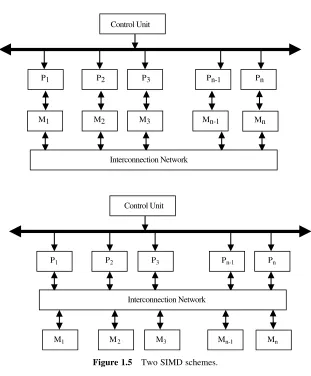
There are two main configurations that have been used in SIMD machines (see Fig. 1.5). In the first scheme, each processor has its own local memory. Processors can communicate with each other through the interconnection network. If the inter-connection network does not provide direct inter-connection between a given pair of processors, then this pair can exchange data via an intermediate processor. The ILLIAC IV used such an interconnection scheme. The interconnection network in the ILLIAC IV allowed each processor to communicate directly with four neighbor-ing processors in an 88 matrix pattern such that theithprocessor can communi-cate directly with the (i21)th, (iþ1)th, (i28)th, and (iþ8)thprocessors. In the second SIMD scheme, processors and memory modules communicate with each other via the interconnection network. Two processors can transfer data between each other via intermediate memory module(s) or possibly via intermediate processor(s). The BSP (Burroughs’ Scientific Processor) used the second SIMD scheme.
1.4 MIMD ARCHITECTURE
Multiple-instruction multiple-data streams (MIMD) parallel architectures are made of multiple processors and multiple memory modules connected together via some
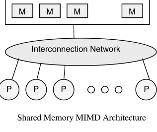
interconnection network. They fall into two broad categories: shared memory or message passing. Figure 1.6 illustrates the general architecture of these two cat-egories. Processors exchange information through their central shared memory in shared memory systems, and exchange information through their interconnection network in message passing systems.
A shared memory system typically accomplishes interprocessor coordination through a global memory shared by all processors. These are typically server sys-tems that communicate through a bus and cache memory controller. The bus/ cache architecture alleviates the need for expensive multiported memories and inter-face circuitry as well as the need to adopt a message-passing paradigm when devel-oping application software. Because access to shared memory is balanced, these systems are also called SMP (symmetric multiprocessor) systems. Each processor has equal opportunity to read/write to memory, including equal access speed.
Control Unit
P1
M1
P2
M2
P3
M3
Pn
Mn
Pn-1
Mn-1
Interconnection Network
Control Unit
P1
M1
P2
M2
P3
M3
Pn
Mn Pn-1
[image:22.441.66.377.54.430.2]Mn-1 Interconnection Network
Commercial examples of SMPs are Sequent Computer’s Balance and Symmetry, Sun Microsystems multiprocessor servers, and Silicon Graphics Inc. multiprocessor servers.
Amessage passing system(also referred to as distributed memory) typically com-bines the local memory and processor at each node of the interconnection network. There is no global memory, so it is necessary to move data from one local memory to another by means of message passing. This is typically done by a Send/Receive pair of commands, which must be written into the application software by a programmer. Thus, programmers must learn the message-passing paradigm, which involves data copying and dealing with consistency issues. Commercial examples of message pas-sing architectures c. 1990 were the nCUBE, iPSC/2, and various Transputer-based systems. These systems eventually gave way to Internet connected systems whereby the processor/memory nodes were either Internet servers or clients on individuals’ desktop.
It was also apparent that distributed memory is the only way efficiently to increase the number of processors managed by a parallel and distributed system. If scalability to larger and larger systems (as measured by the number of processors) was to continue, systems had to use distributed memory techniques. These two forces created a conflict: programming in the shared memory model was easier, and designing systems in the message passing model provided scalability. The
Interconnection Network
P
M
M M M
P P P
Interconnection Network
P P P P
M
M M M
Shared Memory MIMD Architecture
[image:23.441.142.300.71.204.2]Message Passing MIMD Architecture
distributed-shared memory(DSM) architecture began to appear in systems like the SGI Origin2000, and others. In such systems, memory is physically distributed; for example, the hardware architecture follows the message passing school of design, but the programming model follows the shared memory school of thought. In effect, software covers up the hardware. As far as a programmer is concerned, the architecture looks and behaves like a shared memory machine, but a message pas-sing architecture lives underneath the software. Thus, the DSM machine is a hybrid that takes advantage of both design schools.
1.4.1 Shared Memory Organization
A shared memory model is one in which processors communicate by reading and writing locations in a shared memory that is equally accessible by all processors. Each processor may have registers, buffers, caches, and local memory banks as additional memory resources. A number of basic issues in the design of shared memory systems have to be taken into consideration. These include access control, synchronization, protection, and security. Access control determines which process accesses are possible to which resources. Access control models make the required check for every access request issued by the processors to the shared memory, against the contents of the access control table. The latter contains flags that determine the legality of each access attempt. If there are access attempts to resources, then until the desired access is completed, all disallowed access attempts and illegal processes are blocked. Requests from sharing processes may change the contents of the access control table during execution. The flags of the access control with the synchronization rules determine the system’s functionality. Synchroniza-tion constraints limit the time of accesses from sharing processes to shared resources. Appropriate synchronization ensures that the information flows properly and ensures system functionality. Protection is a system feature that prevents pro-cesses from making arbitrary access to resources belonging to other propro-cesses. Shar-ing and protection are incompatible; sharShar-ing allows access, whereas protection restricts it.
The simplest shared memory system consists of one memory module that can be accessed from two processors. Requests arrive at the memory module through its two ports. An arbitration unit within the memory module passes requests through to a memory controller. If the memory module is not busy and a single request arrives, then the arbitration unit passes that request to the memory controller and the request is granted. The module is placed in the busy state while a request is being serviced. If a new request arrives while the memory is busy servicing a previous request, the requesting processor may hold its request on the line until the memory becomes free or it may repeat its request sometime later.
all processors have equal access time to any memory location. The interconnection network used in the UMA can be a single bus, multiple buses, a crossbar, or a multiport memory. In the NUMA system, each processor has part of the shared memory attached. The memory has a single address space. Therefore, any processor could access any memory location directly using its real address. However, the access time to modules depends on the distance to the processor. This results in a nonuniform memory access time. A number of architectures are used to interconnect processors to memory modules in a NUMA. Similar to the NUMA, each processor has part of the shared memory in the COMA. However, in this case the shared memory consists of cache memory. A COMA system requires that data be migrated to the processor requesting it. Shared memory systems will be discussed in more detail in Chapter 4.
1.4.2 Message Passing Organization
Message passing systems are a class of multiprocessors in which each processor has access to its own local memory. Unlike shared memory systems, communications in message passing systems are performed via send and receive operations. Anodein such a system consists of a processor and its local memory. Nodes are typically able to store messages in buffers (temporary memory locations where messages wait until they can be sent or received), and perform send/receive operations at the same time as processing. Simultaneous message processing and problem calculating are handled by the underlying operating system. Processors do not share a global memory and each processor has access to its own address space. The processing units of a message passing system may be connected in a variety of ways ranging from architecture-specific interconnection structures to geographically dispersed networks. The message passing approach is, in principle, scalable to large pro-portions. By scalable, it is meant that the number of processors can be increased without significant decrease in efficiency of operation.
1.5 INTERCONNECTION NETWORKS
Multiprocessors interconnection networks (INs) can be classified based on a number of criteria. These include (1) mode of operation (synchronous versus asynchronous), (2) control strategy (centralized versus decentralized), (3) switching techniques (circuit versus packet), and (4) topology (static versus dynamic).
1.5.1 Mode of Operation
According to the mode of operation, INs are classified assynchronousversus asyn-chronous. In synchronous mode of operation, a single global clock is used by all components in the system such that the whole system is operating in a lock – step manner. Asynchronous mode of operation, on the other hand, does not require a global clock. Handshaking signals are used instead in order to coordinate the operation of asynchronous systems. While synchronous systems tend to be slower compared to asynchronous systems, they are race and hazard-free.
1.5.2 Control Strategy
According to the control strategy, INs can be classified ascentralizedversus decen-tralized.In centralized control systems, a single central control unit is used to over-see and control the operation of the components of the system. In decentralized control, the control function is distributed among different components in the system. The function and reliability of the central control unit can become the bottle-neck in a centralized control system. While the crossbar is a centralized system, the multistage interconnection networks are decentralized.
1.5.3 Switching Techniques
Interconnection networks can be classified according to the switching mechanism as circuit versus packet switching networks. In the circuit switching mechanism, a complete path has to be established prior to the start of communication between a source and a destination. The established path will remain in existence during the whole communication period. In a packet switching mechanism, communication between a source and destination takes place via messages that are divided into smaller entities, called packets. On their way to the destination, packets can be sent from a node to another in a store-and-forward manner until they reach their des-tination. While packet switching tends to use the network resources more efficiently compared to circuit switching, it suffers from variable packet delays.
1.5.4 Topology
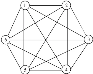
processors and memories. A fully connected topology, for example, is a mapping in which each processor is connected to all other processors in the computer. A ring topology is a mapping that connects processor k to its neighbors, processors (k21) and (kþ1).
In general, interconnection networks can be classified asstaticversusdynamic networks. In static networks, direct fixed links are established among nodes to form a fixed network, while in dynamic networks, connections are established as needed. Switching elements are used to establish connections among inputs and outputs. Depending on the switch settings, different interconnections can be estab-lished. Nearly all multiprocessor systems can be distinguished by their inter-connection network topology. Therefore, we devote Chapter 2 of this book to study a variety of topologies and how they are used in constructing a multiprocessor system. However, in this section, we give a brief introduction to interconnection networks for shared memory and message passing systems.
Shared memory systems can be designed using bus-based or switch-based INs. The simplest IN for shared memory systems is the bus. However, the bus may get saturated if multiple processors are trying to access the shared memory (via the bus) simultaneously. A typical bus-based design uses caches to solve the bus conten-tion problem. Other shared memory designs rely on switches for interconnecconten-tion. For example, a crossbar switch can be used to connect multiple processors to multiple memory modules. A crossbar switch, which will be discussed further in Chapter 2, can be visualized as a mesh of wires with switches at the points of intersection. Figure 1.7 shows (a) bus-based and (b) switch-based shared memory systems. Figure 1.8 shows bus-based systems when a single bus is used versus the case when multiple buses are used.
Message passing INs can be divided into static and dynamic. Static networks form all connections when the system is designed rather than when the connection is needed. In a static network, messages must be routed along established links.
P C
P C
P C
P C
M M M M
Global Memory
P C
P C
P C
(a) (b)
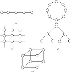
Dynamic INs establish a connection between two or more nodes on the fly as mess-ages are routed along the links. Thenumber of hopsin a path from source to destina-tion node is equal to the number of point-to-point links a message must traverse to reach its destination. In either static or dynamic networks, a single message may have tohopthrough intermediate processors on its way to its destination. Therefore, the ultimate performance of an interconnection network is greatly influenced by the number of hops taken to traverse the network. Figure 1.9 shows a number of popular static topologies: (a) linear array, (b) ring, (c) mesh, (d) tree, (e) hypercube.
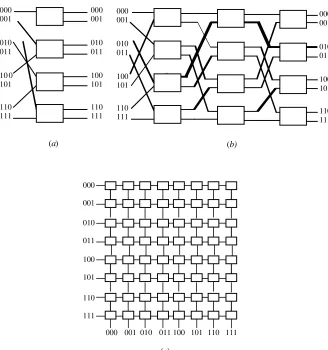
Figure 1.10 shows examples of dynamic networks. The single-stage interconnec-tion network of Figure 1.10ais a simple dynamic network that connects each of the inputs on the left side to some, but not all, outputs on the right side through a single layer of binary switches represented by the rectangles. The binary switches can direct the message on the left-side input to one of two possible outputs on the right side. If we cascade enough single-stage networks together, they form a completely connected multistage interconnection network (MIN), as shown in Figure 1.10b. Theomega MINconnects eight sources to eight destinations. The con-nection from the source 010 to the destination 010 is shown as a bold path in Figure 1.10b. These are dynamic INs because the connection is made on the fly, as needed. In order to connect a source to a destination, we simply use a function of the bits of the source and destination addresses as instructions for dynamically selecting a path through the switches. For example, to connect source 111 to desti-nation 001 in the omega network, the switches in the first and second stage must be set to connect to the upper output port, while the switch at the third stage must be set
P P P
M M M
P P
M M M
P
Figure 1.8 Single bus and multiple bus systems.
Linear Array Ring Mesh Tree Hypercube
to connect to the lower output port (001). Similarly, the crossbar switch of Figure 1.10cprovides a path from any input or source to any other output or destina-tion by simply selecting a direcdestina-tion on the fly. To connect row 111 to column 001 requires only one binary switch at the intersection of the 111 input line and 011 output line to be set.
The crossbar switch clearly uses more binary switching components; for example,N2 components are needed to connectNN source/destination pairs. The omega MIN, on the other hand, connectsNNpairs withN/2 (logN) com-ponents. The major advantage of the crossbar switch is its potential for speed. In one clock, a connection can be made between source and destination. The diameter of the crossbar is one. (Note: Diameter,D, of a network havingNnodes is defined as the maximum shortest paths between any two nodes in the network.) The omega
MIN, on the other hand requires logNclocks to make a connection. The diameter of the omega MIN is therefore logN. Both networks limit the number of alternate paths between any source/destination pair. This leads to limited fault tolerance and net-work traffic congestion. If the single path between pairs becomes faulty, that pair cannot communicate. If two pairs attempt to communicate at the same time along a shared path, one pair must wait for the other. This is calledblocking, and such MINs are calledblocking networks. A network that can handle all possible connec-tions without blocking is called anonblocking network.
Table 1.2 shows a performance comparison among a number of different dynamic INs. In this table,mrepresents the number of multiple buses used, whileNrepresents the number of processors (memory modules) or input/output of the network.
Table 1.3 shows a performance comparison among a number of static INs. In this table, the degree of a network is defined as the maximum number of links (channels) connected to any node in the network. The diameter of a network is defined as the maximum path,p, of the shortest paths between any two nodes. Degree of a node,d, is defined as the number of channels incident on the node. Performance measures will be discussed in more detail in Chapter 3.
1.6 CHAPTER SUMMARY
In this chapter, we have gone over a number of concepts and system configurations related to obtaining high-performance computing via parallelism. In particular, we have provided the general concepts and terminology used in the context of multipro-cessors. The popular Flynn’s taxonomy of computer systems has been provided. An introduction to SIMD and MIMD systems was given. Both shared-memory and the message passing systems and their interconnection networks were introduced. The
TABLE 1.2 Performance Comparison of Some Dynamic INs
Network Delay Cost (Complexity)
Bus O(N) O(1)
Multiple-bus O(mN) O(m)
MINs O(logN) O(NlogN)
TABLE 1.3 Performance Characteristics of Static INs
Network Degree Diameter Cost (#links)
Linear array 2 N21 N21
Binary tree 3 2([log2N]21) N21
n-cube log2N log2N nN/2
rest of the book is organized as follows. In Chapter 2 interconnection networks will be covered in detail. We will study performance metrics in Chapter 3. Shared-memory and message passing architectures are explained in Chapters 4 and 5, respectively. We cover abstract models to study shared memory and message pas-sing systems in Chapter 6. We then study network computing in Chapter 7. Chapters 8 and 9 are dedicated to the parallel virtual machine (PVM) and message passing interface (MPI), respectively. The last chapter gives a comprehensive coverage of the challenging problem of task scheduling and task allocation.
PROBLEMS
1. What has been the trend in computing from the following points of views: (a) cost of hardware;
(b) size of memory; (c) speed of hardware;
(d) number of processing elements; and
(e) geographical locations of system components.
2. Given the trend in computing in the last 20 years, what are your predictions for the future of computing?
3. What is the difference between cluster computing and grid computing? 4. Assume that a switching component such as a transistor can switch in
zero-time. We propose to construct a disk-shaped computer chip with such a com-ponent. The only limitation is the time it takes to send electronic signals from one edge of the chip to the other. Make the simplifying assumption that elec-tronic signals can travel at 300,000 km/s. What is the limitation on the diam-eter of a round chip so that any computation result can by used anywhere on the chip at a clock rate of 1 GHz? What are the diameter restrictions if the whole chip should operate at 1 THz¼1012Hz? Is such a chip feasible? 5. Compare uniprocessor systems with multiprocessor systems for the
follow-ing aspects:
(a) ease of programming; (b) the need for synchronization; (c) performance evaluation; and (d) run time system.
6. Provide a list of the main advantages and disadvantages of SIMD and MIMD machines.
7. Provide a list of the main advantages and disadvantages of shared-memory and message-passing paradigm.
9. Assume that a simple addition of two elements requires a unit time. You are required to compute the execution time needed to perform the addition of a 4040 elements array using each of the following arrangements:
(a) A SIMD system having 64 processing elements connected in nearest-neighbor fashion. Consider that each processor has only its local memory.
(b) A SIMD system having 64 processing elements connected to a shared memory through an interconnection network. Ignore the communication time.
(c) A MIMD computer system having 64 independent elements accessing a shared memory through an interconnection network. Ignore the com-munication time.
(d) Repeat (b) and (c) above if the communication time takes two time units. 10. Conduct a comparative study between the following interconnection
net-works in their cost, performance, and fault tolerance: (a) bus;
(b) hypercube; (c) mesh;
(d) fully connected;
(e) multistage dynamic network; (f) crossbar switch.
REFERENCES
Abraham, S. and Padmanabhan, K. Performance of the direct binary n-cube network for multiprocessors.IEEE Transactions on Computers, 38 (7), 1000 – 1011 (1989).
Agrawal, P., Janakiram, V. and Pathak, G. Evaluating the performance of multicomputer configurations.IEEE Transaction on Computers, 19 (5), 23 – 27 (1986).
Almasi, G. and Gottlieb, A.Highly Parallel Computing, Benjamin Cummings, 1989. Al-Tawil, K., Abd-El-Barr, M. and Ashraf, F. A survey and comparison of wormhole routing
techniques in mesh networks.IEEE Network, March/April 1997, 38 – 45 (1997). Bhuyan, L. N. (ed.) Interconnection networks for parallel and distributed processing.
Computer(Special issue), 20 (6), 9 – 75 (1987).
Bhuyan, L. N., Yang, Q. and Agrawal, D. P. Performance of multiprocessor interconnection networks.Computer, 22 (2), 25 – 37 (1989).
Chen, W.-T. and Sheu, J.-P. Performance analysis of multiple bus interconnection networks with hierarchical requesting model.IEEE Transactions on Computers, 40 (7), 834 – 842 (1991).
Dasgupta, S. Computer Architecture: A Modern Synthesis, vol. 2; Advanced Topics, John Wiley, 1989.
Dongarra, J.Experimental Parallel Computing Architectures, North-Holland, 1987. Duncan, R. A survey of parallel computer architectures.Computer, 23 (2), 5 – 16 (1990). El-Rewini, H. and Lewis, T. G.Distributed and Parallel Computing, Manning & Prentice
Hall, 1998.
Flynn.Computer Architecture: Pipelined and Parallel Processor Design, Jones and Bartlett, 1995.
Goodman, J. R. Using cache memory to reduce processor-memory traffic.Proceedings 10th Annual Symposium on Computer Architecture, June 1983, pp. 124 – 131.
Goyal, A. and Agerwala, T. Performance analysis of future shared storage systems.IBM Journal of Research and Development, 28 (1), 95 – 107 (1984).
Hennessy, J. and Patterson, D.Computer Architecture: A Quantitative Approach, Morgan Kaufmann, 1990.
Hwang, K. and Briggs, F. A.Computer Architecture and Parallel Processing, McGraw-Hill, 1984.
Ibbett, R. N. and Topham, N. P.Architecture of High Performance Computers II, Springer-Verlag, 1989.
Juang, J.-Y. and Wah, B. A contention-based bus-control scheme for multiprocessor systems. IEEE Transactions on Computers, 40 (9), 1046 – 1053 (1991).
Lewis, T. G. and El-Rewini, H.Introduction to Parallel Computing, Prentice-Hall, 1992. Linder, D. and Harden, J. An adaptive and fault tolerant wormhole routing strategy fork-ary
n-cubes.IEEE Transactions on Computers, 40 (1), 2 – 12 (1991).
Moldovan, D. Parallel Processing, from Applications to Systems, Morgan Kaufmann Publishers, 1993.
Ni, L. and McKinely, P. A survey of wormhole routing techniques in direct networks.IEEE Computer, February 1993, 62 – 76 (1993).
Patel, J. Performance of processor – memory interconnections for multiprocessor computer systems.IEEE Transactions, 28 (9), 296 – 304 (1981).
Reed, D. and Fujimoto, R. Multicomputer Networks:Message-Based Parallel Processing, MIT Press, 1987.
Serlin, O.The Serlin Report On Parallel Processing, No. 54, pp. 8 – 13, November 1991. Sima, E., Fountain, T. and Kacsuk, P.Advanced Computer Architectures: A Design Space
Approach, Addison-Wesley, 1996.
Stone, H.High-Performance Computer Architecture, 3rd ed., Addison-Wesley, 1993. The Accelerated Strategic Computing Initiative Report, Lawrence Livermore National
Laboratory, 1996.
Wilkinson, B.Computer Architecture: Design and Performance, 2nd ed., Prentice-Hall, 1996. Yang, Q. and Zaky, S. Communication performance in multiple-bus systems.IEEE
Trans-actions on Computers, 37 (7), 848 – 853 (1988).
Youn, H. and Chen, C. A comprehensive performance evaluation of crossbar networks.IEEE Transactions on Parallel and Distribute Systems, 4 (5), 481 – 489 (1993).
Multiprocessors Interconnection
Networks
As we have seen in Chapter 1, a multiprocessor system consists of multiple processing units connected via some interconnection network plus the software needed to make the processing units work together. There are two major factors used to categorize such systems: the processing units themselves, and the intercon-nection network that ties them together. A number of communication styles exist for multiprocessing networks. These can be broadly classified according to the com-munication model as shared memory (single address space) versus message passing (multiple address spaces). Communication in shared memory systems is performed by writing to and reading from the global memory, while communication in message passing systems is accomplished via send and receive commands. In both cases, the interconnection network plays a major role in determining the communication speed. In this chapter, we introduce the different topologies used for interconnecting multiple processors and memory modules. Two schemes are introduced, namely static and dynamic interconnection networks. Static networks form all connections when the system is designed rather than when the connection is needed. In a static network, messages must be routed along established links. Dynamic interconnection networks establish connections between two or more nodes on the fly as messages are routed along the links. The hypercube, mesh, andk-aryn-cube topologies are introduced as examples for static networks. The bus, crossbar, and multistage inter-connection topologies are introduced as examples for dynamic interinter-connection net-works. Our coverage in this chapter will conclude with a section on performance evaluation and analysis of the different interconnection networks.
2.1 INTERCONNECTION NETWORKS TAXONOMY
In this section, we introduce a topology-based taxonomy for interconnection networks (INs). An interconnection network could be either static or dynamic. Con-nections in a static network are fixed links, while conCon-nections in a dynamic network
19
are established on the fly as needed. Static networks can be further classified accord-ing to their interconnection pattern as one-dimension (1D), two-dimension (2D), or hypercube (HC). Dynamic networks, on the other hand, can be classified based on interconnection scheme as bus-based versus switch-based. Bus-based networks can further be classified as single bus or multiple buses. Switch-based dynamic net-works can be classified according to the structure of the interconnection network as single-stage (SS), multistage (MS), or crossbar networks. Figure 2.1 illustrate this taxonomy. In the following sections, we study the different types of dynamic and static interconnection networks.
2.2 BUS-BASED DYNAMIC INTERCONNECTION NETWORKS
2.2.1 Single Bus Systems
A single bus is considered the simplest way to connect multiprocessor systems. Figure 2.2 shows an illustration of a single bus system. In its general form, such a system consists of N processors, each having its own cache, connected by a
Figure 2.1 A topology-based taxonomy for interconnection networks.
shared bus. The use of local caches reduces the processor – memory traffic. All pro-cessors communicate with a single shared memory. The typical size of such a system varies between 2 and 50 processors. The actual size is determined by the traffic per processor and the bus bandwidth (defined as the maximum rate at which the bus can propagate data once transmission has started). The single bus network complexity, measured in terms of the number of buses used, isO(1), while the time complexity, measured in terms of the amount of input to output delay isO(N).
Although simple and easy to expand, single bus multiprocessors are inherently limited by the bandwidth of the bus and the fact that only one processor can access the bus, and in turn only one memory access can take place at any given time. The characteristics of some commercially available single bus computers are summarized in Table 2.1.
2.2.2 Multiple Bus Systems
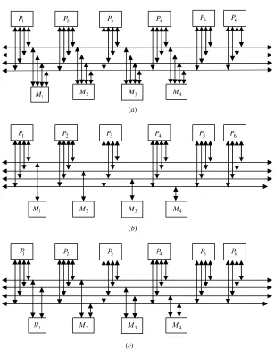
The use of multiple buses to connect multiple processors is a natural extension to the single shared bus system. A multiple bus multiprocessor system uses several parallel buses to interconnect multiple processors and multiple memory modules. A number of connection schemes are possible in this case. Among the possibilities are the multiple bus with full bus – memory connection (MBFBMC), multiple bus with single bus memory connection (MBSBMC), multiple bus with partial bus – memory connection (MBPBMC), and multiple bus with class-based memory connection (MBCBMC). Illustrations of these connection schemes for the case of N¼6 processors, M¼4 memory modules, and B¼4 buses are shown in Figure 2.3. The multiple bus with full bus – memory connection has all memory modules connected to all buses. The multiple bus with single bus – memory connec-tion has each memory module connected to a specific bus. The multiple bus with partial bus – memory connection has each memory module connected to a subset of buses. The multiple bus with class-based memory connection has memory mod-ules grouped into classes whereby each class is connected to a specific subset of buses. A class is just an arbitrary collection of memory modules.
One can characterize those connections using the number of connections required and the load on each bus as shown in Table 2.2. In this table, k represents the number of classes;grepresents the number of buses per group, andMjrepresents the number of memory modules in classj.
TABLE 2.1 Characteristics of Some Commercially Available Single Bus Systems
Machine Name
Maximum No. of
Processors Processor
Clock Rate
Maximum
Memory Bandwidth
HP 9000 K640 4 PA-8000 180 MHz 4,096 MB 960 MB/s
IBM RS/6000 R40 8 PowerPC 604 112 MHz 2,048 MB 1,800 MB/s
In general, multiple bus multiprocessor organization offers a number of desirable features such as high reliability and ease of incremental growth. A single bus failure will leave (B21) distinct fault-free paths between the processors and the memory modules. On the other hand, when the number of buses is less than the number of memory modules (or the number of processors), bus contention is expected to increase.
P P P P P P
M M M M
a
P P P P P P
M M
M M
b
[image:37.441.66.374.164.555.2]c
2.2.3 Bus Synchronization
A bus can be classified as synchronous orasynchronous. The time for any trans-action over a synchronous bus is known in advance. In accepting and/or generating information over the bus, devices take the transaction time into account. Asynchro-nous bus, on the other hand, depends on the availability of data and the readiness of devices to initiate bus transactions.
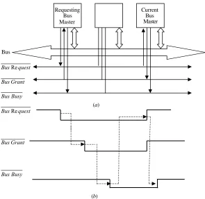
In a single bus multiprocessor system, bus arbitration is required in order to resolve the bus contention that takes place when more than one processor competes to access the bus. In this case, processors that want to use the bus submit their requests to bus arbitration logic. The latter decides, using a certain priority scheme, which processor will be granted access to the bus during a certain time interval (bus master). The process of passing bus mastership from one processor to another is calledhandshaking and requires the use of two control signals:bus requestandbus grant. The first indicates that a given processor is requesting master-ship of the bus, while the second indicates that bus mastermaster-ship is granted. A third signal, calledbus busy, is usually used to indicate whether or not the bus is currently being used. Figure 2.4 illustrates such a system.
In deciding which processor gains control of the bus, the bus arbitration logic uses a predefined priority scheme. Among the priority schemes used are random
d
Figure 2.3 Continued.
TABLE 2.2 Characteristics of Multiple Bus Architectures
Connection Type No. of Connections Load on Busi
MBFBMC B(NþM) NþM
MBSBMC BNþM NþMj
MBPBMC B(NþM/g) NþM/g
MBCBMC BNþPkj¼1Mj(jþBk) Nþ
Pk
priority, simple rotating priority, equal priority, and least recently used (LRU) pri-ority. After each arbitration cycle, in simple rotating priority, all priority levels are reduced one place, with the lowest priority processor taking the highest priority. In equal priority, when two or more requests are made, there is equal chance of any one request being processed. In the LRU algorithm, the highest priority is given to the processor that has not used the bus for the longest time.
2.3 SWITCH-BASED INTERCONNECTION NETWORKS
In this type of network, connections among processors and memory modules are made using simple switches. Three basic interconnection topologies exist:crossbar, single-stage, andmultistage.
2.3.1 Crossbar Networks
Acrossbar networkrepresents the other extreme to the limited single bus network. While the single bus can provide only a single connection, the crossbar can provide
Requesting Current Bus Bus
Master Master
Bus
quest BusRe
Grant Bus
Busy Bus
(a) quest
BusRe
Grant Bus
Busy Bus
[image:39.441.71.366.63.350.2](b)
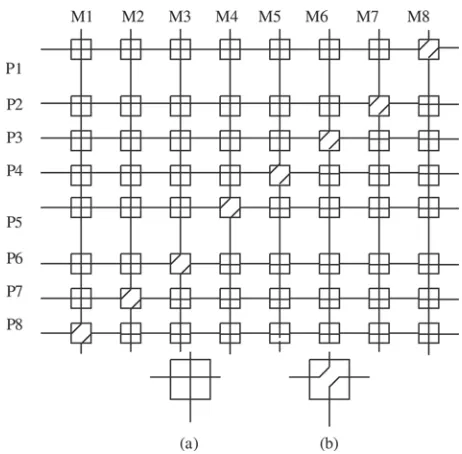
simultaneous connections among all its inputs and all its outputs. The crossbar contains a switching element (SE) at the intersection of any two lines extended horizontally or vertically inside the switch. Consider, for example the 88 crossbar network shown in Figure 2.5. In this case, an SE (also called a cross-point) is pro-vided at each of the 64 intersection points (shown as small squares in Fig. 2.5). The figure illustrates the case of setting the SEs such that simultaneous connections between Pi andM8iþ1 for 1i8 are made. The two possible settings of an SE in the crossbar (straight and diagonal) are also shown in the figure.
As can be seen from the figure, the number of SEs (switching points) required is 64 and the message delay to traverse from the input to the output is constant, regard-less of which input/output are communicating. In general for anNNcrossbar, the network complexity, measured in terms of the number of switching points, isO(N2) while the time complexity, measured in terms of the input to output delay, isO(1). It should be noted that the complexity of the crossbar network pays off in the form of reduction in the time complexity. Notice also that the crossbar is anonblocking net-work that allows a multiple input – output connection pattern (permutation) to be achieved simultaneously. However, for a large multiprocessor system the complex-ity of the crossbar can become a dominant financial factor.
2.3.2 Single-Stage Networks
[image:40.441.105.336.360.587.2]In this case, a single stage of switching elements (SEs) exists between the inputs and the outputs of the network. The simplest switching element that can be used is the
22 switching element (SE). Figure 2.6 illustrates the four possible settings that an SE can assume. These settings are calledstraight,exchange,upper-broadcast, and lower-broadcast. In the straight setting, the upper input is transferred to the upper output and the lower input is transferred to the lower output. In the exchange setting the upper input is transferred to the lower output and the lower input is transferred to the upper output. In the upper-broadcast setting the upper input is broadcast to both the upper and the lower outputs. In the lower-broadcast the lower input is broadcast to both the upper and the lower outputs.
To establish communication between a given input (source) to a given output (destination), data has to be circulated a number of times around the network. A well-known connection pattern for interconnecting the inputs and the outputs of a single-stage network is the Shuffle–Exchange. Two operations are used. These can be defined using an m bit-wise address pattern of the inputs, pm1pm2. . .p1p0, as follows:
S(pm1pm2. . .p1p0)¼pm2pm3. . .p1p0pm1
E(pm1pm2. . .p1p0)¼pm1pm2. . .p1p0
With shuffle (S) and exchange (E) operations, data is circulated from input to output until it reaches its destination. If the number of inputs, for example, pro-cessors, in a single-stageINisNand the number of outputs, for example, memories, isN, the number of SEs in a stage isN/2. The maximum length of a path from an input to an output in the network, measured by the number of SEs along the path, is log2N.
Example In an 8-input single stageShuffle –Exchangeif the source is 0 (000) and the destination is 6 (110), then the following is the required sequence ofShuffle/ Exchangeoperations and circulation of data:
E(000)!1(001)!S(001)!2(010)!E(010)!3(011)!S(011)!6(110)
The network complexity of the single-stage interconnection network isO(N) and the time complexity isO(N).
In addition to the shuffle and the exchange functions, there exist a number of other interconnection patterns that are used in forming the interconnections among stages in interconnection networks. Among these are the Cube and the Plus-Minus2i(PM2I) networks. These are introduced below.
Straight Exchange Upper-broadcast Lower-broadcast
The Cube Network The interconnection pattern used in the cube network is defined as follows:
Ci(pm1pm2 piþ1pipi1 p1p0)¼pm1pm2 piþ1pipi1 p1p0
Consider a 3-bit address (N¼8), then we haveC2(6)¼2,C1(7)¼5 andC0(4)¼5. Figure 2.7 shows the cube interconnection patterns for a network withN¼8.
The network is called the cube network due to the fact that it resembles the interconnection among the corners of an n-dimensional cube (n¼log2N) (see Fig. 2.16e, later).
The Plus – Minus 2i(PM2I) Network The PM2I network consists of 2k inter-connection functions defined as follows:
PM2þi(P)¼Pþ2imodN(0i,k)
PM2i(P)¼P2imodN(0i,k)
For example, consider the caseN¼8,PM2þ1(4)¼4þ21 mod 8¼6. Figure 2.8 shows the PM2I for N¼8. It should be noted that PM2þ(k1)(P)¼
PM2(k1)(P)8P, 0P,N. It should also be noted that PM2þ2¼C2. This last observation indicates that it should be possible to use the PM2I network to perform at least part of the connections that are parts of the Cube network (simulating the Cube network using the PM2I network) and the reverse is also possible. Table 2.3 provides the lower and the upper bounds on network simulation times for the three networks PM2I, Cube, and Shuffle – Exchange. In this table the entries at the intersection of a given row and a given column are the lower and the upper
bounds on the time required for the network in the row to simulate the network in the column (see the exercise at the end of the chapter).
The Butterfly Function The interconnection pattern used in the butterfly network is defined as follows:
B(pm1pm2 p1p0)¼p0pm2 p1pm1
Consider a 3-bit address (N¼8), the following is the butterfly mapping:
B(000)¼000 B(001)¼100
a
b
c
Figure 2.8 The PM2I network forN¼8 (a),PM2þ0forN¼8; (b)PM2þ1forN¼8; and
(c)PM2þ2forN¼8.
TABLE 2.3 Network Simulation Time for Three Networks
Simulation Time PM2I Cube Shuffle – Exchange
PM2I Lower 1 2 k
Upper 1 2 kþ1
Cube Lower k 1 k
Upper k 1 k
Shuffle – Exchange Lower 2k21 kþ1 1
B(010)¼010 B(011)¼110 B(100)¼001 B(101)¼101 B(110)¼011 B(111)¼111
2.3.3 Multistage Networks
Multistage interconnection networks (MINs) were introduced as a means to improve some of the limitations of the single bus system while keeping the cost within an affordable limit. The most undesirable single bus limitation that MINs is set to improve is the availability of only one single path between the processors and the memory modules. Such MINs provide a number of simultaneous paths between the processors and the memory modules.
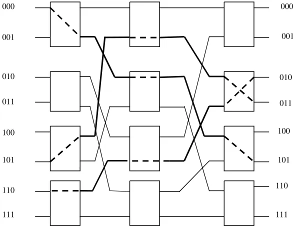
As shown in Figure 2.9, a general MIN consists of a number of stages each con-sisting of a set of 22 switching elements. Stages are connected to each other using Inter-stage Connection (ISC) Pattern. These patterns may follow any of the routing functions such as Shuffle – Exchange, Butterfly, Cube, and so on.
Figure 2.10 shows an example of an 88 MIN that uses the 22 SEs described before. This network is known in the literature as theShuffle–Exchange network (SEN). The settings of the SEs in the figure illustrate how a number of paths can be established simultaneously in the network. For example, the figure shows how three simultaneous paths connecting the three pairs of input/output 000!101, 101!011, and 110!010 can be established. It should be noted that the intercon-nection pattern among stages follows theshuffleoperation.
In MINs, the routing of a message from a given source to a given destination is based on the destination address (self-routing). There exist log2N stages in an
Switches Switches Switches
ISC 1
ISC x-1
NNMIN. The number of bits in any destination address in the network is log2N. Each bit in the destination address can be used to route the message through one stage. The destination address bits are scanned from left to right and the stages are traversed from left to right. The first (most significant bit) is used to control the routing in the first stage; the next bit is used to control the routing in the next stage, and so on. The convention used in routing messages is that if the bit in the destination address controlling the routing in a given stage is 0, then the message is routed to the upper output of the switch. On the other hand if the bit is 1, the mess-age is routed to the lower output of the switch. Consider, for example, the routing of a message from source input 101 to destination output 011 in the 88 SEN shown in Figure 2.10. Since the first bit of the destination address is 0, therefore the mess-age is first routed to the upper output of the switch in the first (leftmost) stmess-age. Now, the next bit in the destination address is 1, thus the message is routed to the lower output of the switch in the middle stage. Finally, the last bit is 1, causing the message to be routed to the lower output in the switch in the last stage. This sequence causes the message to arrive at the correct output (see Fig. 2.10). Ease of message routing in MINs is one of the most desirable features of these networks.
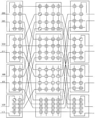
[image:45.441.69.362.66.297.2]The Banyan Network A number of other MINs exist, among these the Banyan network is well known. Figure 2.11 shows an example of an 88 Banyan network. The reader is encouraged to identify the basic features of the Banyan network.
If the number of inputs, for example, processors, in an MIN isNand the number of outputs, for example, memory modules, isN, the number of MIN stages is log2N and the number of SEs per stage is N/2, and hence the network complexity, measured in terms of the total number of SEs is O(Nlog2N). The number of SEs along the path is usually taken as a measure of the delay a message has to encounter as it finds its way from a source input to a destination output. The time complexity, measured by the number of SEs along the path from input to output, isO(log2N). For example, in a 1616 MIN, the length of the path from input to output is 4. The total number of SEs in the network is usually taken as a measure for the total area of the network. The total area of a 1616 MIN is 32 SEs.
The Omega Network The Omega Network represents another well-known type of MINs. A sizeN omega networkconsists ofn(n¼log2Nsingle-stage) Shuffle – Exchange networks. Each stage consists of a column ofN=2, two-input switching elements whose input is a shuffle connection. Figure 2.12 illustrates the case of an N¼8 Omega network. As can be seen from the figure, the inputs to each stage follow the shuffle interconnection pattern. Notice that the connections are identical to those used in the 88 Shuffle – Exchange network (SEN) shown in Figure 2.10.
Owing to its versatility, a number of university projects as well as commercial MINs have been built. These include the Texas Reconfigurable Array Computer (TRAC) at the University of Texas at Austin, theCedarat the University of Illinois at Urbana-Champaign, theRP3at IBM, theButterflyby BBN Laboratories, and the NYU Ultracomputer at New York University. The NYU Ultracomputer is an exper-imental shared memory MIMD architecture that could have as many as 4096 pro-cessors connected through an Omega MIN to 4096 memory modules. The MIN is an enhanced network that can combine two or more requests bound for the same memory address. The network interleaves consecutive memory addresses across the memory modules in order to reduce conflicts in accessing different data