Robust Moving Object Detection by
Information Fusion from Multiple Cameras
Thesis submitted in accordance with the requirements of the
University of Liverpool for the degree of
Doctor in Philosophy
Jie REN
January 2014
ABSTRACT
Moving object detection is an essential process before tracking and event recognition in video surveillance can take place. To monitor a wider field of view and avoid occlusions in pedestrian tracking, multiple cameras are usually used and homography can be employed to associate multiple camera views. Foreground regions detected from each of the multiple camera views are projected into a virtual top view according to the homography for a plane. The intersection regions of the foreground projections indicate the locations of moving objects on that plane. The homography mapping for a set of parallel planes at different heights can increase the robustness of the detection. However, homography mapping is very time consuming and the intersections of non-corresponding foreground regions can cause false-positive detections.
In this thesis, a real-time moving object detection algorithm using multiple cameras is proposed. Unlike the pixelwise homography mapping which projects binary foreground images, the approach used in the research described in this thesis was to approximate the contour of each foreground region with a polygon and only transmit and project the polygon vertices. The foreground projections are rebuilt from the projected polygons in the reference view. The experimental results have shown that this method can be run in real time and generate results similar to those using foreground images.
TABLE OF CONTENTS
ABSTRACT ... i
TABLE OF CONTENTS ... i
LIST OF FIGURES ... v
LIST OF TABLES ... viii
Acknowledgements ... xi
1
INTRODUCTION ... 1
1.1 Visual Surveillance and Moving Object Detection ... 1
1.2 Aims and Objectives ... 4
1.2.1 Real-time Foreground Projection with Homography ... 5
1.2.2 False Positives in the Detection ... 6
1.3 Organization of the Thesis ... 6
1.4 Contributions ... 7
2.
Literature Review ... 8
2.1 A Review of Multi-Camera Visual Surveillance ... 8
2.1.1 Low-degree Information Fusion ... 8
2.1.2 Intermediate-degree Information Fusion ... 9
2.1.3 High-degree Information Fusion ... 10
2.2 A Review of Multi-View Association ... 11
2.2.1 Central Projections ... 11
2.2.2 Epipolar Lines ... 12
2.2.3 Planar Homographies ... 13
2.3 A Review of Foreground Fusion with Homographies ... 13
2.3.1 Foreground Pixel-based Methods ... 13
2.3.2 Foreground Line-based Methods ... 14
2.3.3 Foreground Region-based Methods ... 14
2.4 A Review of Colour Matching ... 14
2.5 A Review of Phantom Removal ... 15
2.6 Summary ... 17
3
HOMOGRAPHY ESTIMATION ... 18
3.2 An Introduction to Homography ... 21
3.3 Estimation of Planar Homography ... 21
3.3.1 Point Correspondences ... 22
3.3.2 Robust Estimation ... 23
3.3.3 Camera Calibration ... 24
3.4 Estimation of Multi-Plane Homographies ... 24
3.4.1 Calibration ... 24
3.4.2 Vanishing Point... 25
3.5 Experiments and Analysis ... 26
3.5.1 Experimental Results of the PETS’2001 ... 26
3.5.2 Experimental Results of the Campus Dataset ... 27
3.6 Summary ... 31
4
MOVING OBJECT DETECTION WITH REAL-TIME FUSION ... 33
4.1 Foreground Segmentation in a Single View ... 34
4.1.1 Introduction to Foreground Segmentation ... 34
4.1.2 Gaussian Mixture Models ... 36
4.2 Foreground Regions ... 37
4.2.1 Connected Component Analysis ... 37
4.2.2 Morphological Processing ... 37
4.2.3 Post-processing ... 39
4.3 Foreground Polygons ... 39
4.3.1 Contour Extraction ... 39
4.3.2 Polygon Approximation ... 40
4.4 Foreground Projection ... 41
4.4.1 Polygon Projection ... 41
4.4.2 Reconstruction of the Projected Foreground ... 42
4.5 Foreground Fusion ... 44
4.5.1 Fusion with Multiple Views ... 44
4.5.2 Fusion with Multi-Plane Homographies ... 45
4.6 Experimental Results ... 46
4.6.1 Experimental Results of the Campus Dataset ... 47
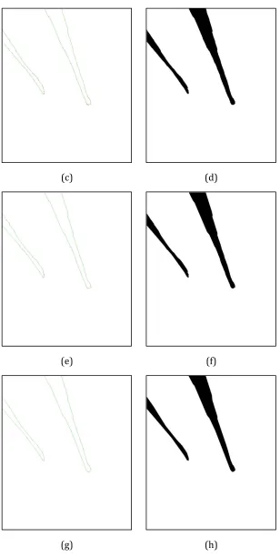
4.6.1.1 Foreground Polygons ... 47
4.6.1.2 Polygon Projections ... 50
4.6.1.3 Projected Foreground Fusion based on a Single Plane ... 53
5
PHANTOM REMOVAL WITH GEOMETRICAL INFOMATION ... 62
5.1 Introduction to Phantoms ... 62
5.2 Region Based Foreground Fusion ... 65
5.3 Warped Back Patches in a Single View ... 68
5.4 Height Matching in a Single View ... 68
5.4.1 Normalized Distances ... 68
5.4.2 Height Matching of a Patch Set ... 69
5.5 Patch Classification in a Single View ... 70
5.5.1 Position Analysis ... 70
5.5.2 Patch Classification in a Single View ... 70
5.6 Height Matching in the Top View ... 71
5.7 Experimental Results ... 74
5.7.1 Intersection Region Analysis ... 75
5.7.2 Phantom Pruning with Height Matching ... 76
5.7.3 Evaluations ... 84
5.8 Summary ... 85
6
PHANTOM REMOVAL WITH HEIGHTS AND COLOUR CUES ... 87
6.1 Colour Spaces ... 87
6.1.1 The RGB and rgb Models ... 87
6.1.2 The HSI Model ... 88
6.2 Colour Matching Methods ... 89
6.2.1 Template Matching ... 90
6.2.2 Histogram Based Colour Matching ... 90
6.2.3 Mahalanobis Distance Based Colour Matching ... 90
6.3 Appearance Matching ... 91
6.3.1 Torso Regions ... 91
6.3.2 Appearance Models ... 91
6.3.3 Colour Matching ... 94
6.4 Phantom Removal Based on Heights and Colours ... 96
6.4.1 Height Matching ... 98
6.4.2 Colour Matching ... 98
6.4.3 Patch Classification in a Single View ... 98
6.4.4 Region Classification in the Top View ... 99
6.5 Experimental Results ... 101
6.5.1 Phantom Removal with Colour Matching ... 101
6.5.2 Phantom Removal Based on Heights and Colours ... 110
6.5.3 Discussions ... 121
7
CONCLUSIONS AND FUTURE WORK ... 123
APPENDIX ... 126
A. 1 Publication List ... 126
LIST OF FIGURES
Figure 1.1 A schematic diagram of a typical intelligent visual surveillance system with a single camera. ... 2 Figure 1.2 A schematic diagram of a multi-camera approach with high-degree
information fusion... 3 Figure 1.3 A schematic diagram of the phantom occurrence in multi-view
detection via homography mapping of foregrounds. ... 6 Figure 3.1 The geometry of a pinhole camera. ... 18 Figure 3.2 Procedure for the homography estimation in the PETS’2001 dataset. ... 28 Figure 3.3 The landmark points collected in two camera views and a virtual top
view. ... 29 Figure 3.4 Fusion of the projected background images in the top view. ... 31 Figure 3.5 Warped back points corresponding to the selected points in Figure
3.3(e). ... 31 Figure 4.1 Schematic diagram of dilation and erosion. ... 38 Figure 4.2 The polygon approximation for a foreground region. ... 41 Figure 4.3 The ray-casting algorithm to decide whether a given point is inside a
polygon. ... 42 Figure 4.4 Schematic diagram of the homography projection according to the
ground plane. ... 44 Figure 4.5 Schematic diagram of the overlaid foreground projections and the
intersection region. ... 45 Figure 4.6 Schematic diagram of the homography projection according to the
ground plane and a plane parallel to the ground plane. ... 46 Figure 4.7 The foreground polygon approximation at frame 1020 in camera
view a... 48 Figure 4.8 Foreground projection using the bitmap method at frame 1020 in
camera view a. ... 51 Figure 4.9 Results of the foreground polygon projection at frame 1020 in
Figure 4.10 Fusion of the foreground projections according to the homographies for a set of parallel planes at different heights. ... 54 Figure 4.11 Overlaid foreground projections from two camera views and with
multi-plane homographies. ... 56 Figure 4.12 Intersection regions identified with differnet thresholds at
frames 810, 1270, and 2385. ... 57 Figure 4.13 Foreground detections and the foreground polygons in two camera
views. ... 59 Figure 4.14 Moving object detection by the foreground fusion for multi-planes
homographies. ... 59 Figure 5.1 A schematic diagram of phantom occurrence using ground-plane
homography. ... 63 Figure 5.2 Examples of missed intersections by using ground-plane homography mapping. ... 64 Figure 5.3 A schematic diagram of the homography mapping according to plane
p. ... 65 Figure 5.4 An example of the projected foreground intersections due to the
same object by using the homographies for a set of planes at different heights. ... 66 Figure 5.5 An example of the warped back foreground intersections in two
camera views. ... 67 Figure 5.6 A schematic diagram of height matching in a camera view. ... 69 Figure 5.7 A schematic diagram of position analysis in a camera view... 70 Figure 5.8 A schematic diagram of the position analysis in two camera views.. ... 72 Figure 5.9 The ground-truth number of objects (the first curve) and the
numbers of the detected foreground regions in two camera views (the second and third curve). ... 75 Figure 5.10 The number of the detected intersection regions (the first curve),
the number of the expected intersection regions (the second curve), and the difference between these two curves (the third curve). ... 76 Figure 5.11 The process of phantom removal using height matching at frame
Figure 5.13 The process of phantom removal using height matching at frame 1335. ... 81 Figure 5.14 Classification results of the intersection regions at frame 1335
using height matching. ... 83 Figure 6.1 HSI colour space. ... 89 Figure 6.2 A flowchart of the proposed phantom removal algorithm based on heights and colours. ... 97 Figure 6.3 The process of the phantom removal algorithm using colour cues at
frame 1320. ... 102 Figure 6.4 The colour clustering results of the pedestrian with the red jacket at
frame 1320. ... 103 Figure 6.5 The colour distributions of the torso regions in the hue-and-saturation plane at frame 1320. ... 104 Figure 6.6 Classification results of the intersection regions at frame 1320. ... 107 Figure 6.7 The process of phantom removal using the height matching and
colour matching at frame 1200. ... 111 Figure 6.8 Classification results of the intersection regions at frame 1200 using
both height matching and colour matching. ... 114 Figure 6.9 The process of the phantom removal using height matching and
colour matching at frame 2115. ... 115 Figure 6.10 Classification results of the intersection regions at frame 2115
using both height matching and colour matching and only the height matching. ... 118 Figure 6.11 Comparison of classification errors between height matching and
LIST OF TABLES
Table 3.1 The intrinsic parameters of the two cameras in campus dataset. ... 30 Table 3.2 The extrinsic parameters of the two cameras in campus dataset. ... 30 Table 4.1 The processing speeds for the contour, polygon approximations (with
different distance 𝜀) and the bounding box method. ... 49 Table 4.2 The accuracy of the contour, polygon approximations (with different distance 𝜀) and the bounding box method. ... 50 Table 4.3 The projection accuracy of the contour, polygon projection (with
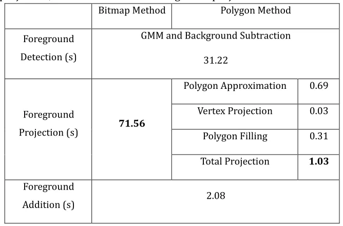
different 𝜀) and the bounding box method. ... 53 Table 4.4 Execution times for running the bitmap projection and the polygon
projection, the total time for the foreground projections are in bold font.55 Table 4.5 The accuracy of the polygon projection method. ... 60 Table 4.6 Execution times for running different algorithms on one camera, the
total time for the foreground projections and fusions are in bold font. ... 60 Table 5.1 Classification of the intersection regions from two camera views. .... 71 Table 5.2 Height matching at frame 1200 in camera view a, the data in bold is the smallest normalized distance in each patch set. ... 79 Table 5.3 Height matching at frame 1200 in camera view b, the data in bold is
the smallest normalized distance in each patch set. ... 79 Table 5.4 The results of regions classification using height matching. ... 80 Table 5.5 The height matching at frame 1335 in camera view a, the data in bold
is the smallest normalized distance in each patch set... 82 Table 5.6 The height matching at frame 1335 in camera view b, the data in bold
is the smallest normalized distance in each patch set... 83 Table 5.7 The classification results of the foreground intersections at frame
Table 6.2 The clustering results of the pedestrian with a red coat in Figure 6.3 (g) in terms of the RGB space and the transformed values in the HSI space. ... 103 Table 6.3 The clustering results of the torso regions in both camera views, the
data in bold indicates the hue value of each selected cluster in the colour matching. ... 105 Table 6.4 The colour matching results in camera view a, the data in bold
indicates the matched foreground region in each patch set. ... 106 Table 6.5 The colour matching results in camera view b, the data in bold
indicates the matched foreground region in each patch set. ... 107 Table 6.6 Classification results with colour matching (HSI) when compared
with ground truth. ... 108 Table 6.7 The false negative rate and the false positive rate of the classification
with colour matching. ... 108 Table 6.8 The false negative rate and the false positive rate of the classification
with colour matching using RGB space. ... 109 Table 6.9 Height matching and colour matching at frame 1200 in camera view a,
the data in bold indicates the matched foreground region and its corresponding normalized distance and colour distance in each patch set. ... 112 Table 6.10 Height matching and colour matching at frame 1200 in camera view
b, the data in bold indicates the matched foreground region and its corresponding normalized distance and colour distance in each patch set. ... 113 Table 6.11 Classification results for the foreground intersections at frame 1200
using both height matching and colour matching. ... 113 Table 6.12 Height matching and colour matching at frame 2115 in camera view
a, the data in bold indicates the matched foreground region and its corresponding normalized distance, colour distance and classification result in each patch set. ... 116 Table 6.13 Height matching and colour matching at frame 2115 in camera view
b, the data in bold indicates the matched foreground region and its corresponding normalized distance, colour distance and classification result in each patch set. ... 117 Table 6.14 Classification results of the foreground intersections at frame 2115
Table 6.15 Performance evaluation of the classification using the height matching and colour matching. ... 119 Table 6.16 The classification errors with height matching and colour matching. ... 119 Table 6.17 Computation costs of the height matching, colour matching and
Acknowledgements
I would like to thank my supervisors Prof. Jeremy S. Smith and Dr. Ming Xu. Without their patience and support in supervising my research and revising this thesis, I would have been unable to complete the work for my PhD.
I am very grateful to Xi'an Jiaotong-Liverpool University for providing a PhD studentship and a living allowance to me. I would like to thank the support of the National Natural Science Foundation of China (NSFC) under Grant 60975082 and the Natural Science Foundation of Jiangsu Province, China, under Grant BK2008180.
I am thankful to Dr. Shi Cheng, Dr. Jimin Xiao and Mr. Yungang Zhang for their advice on programming. I am also grateful to Mr. Chili Li and Mr. Yuyao Yan for their reviewing of my reports and thesis.
I want to thank the classmates and colleagues who helped and supported me in my study: Ms. Guifen Wang, Ms. Yanfei Qi, Mr. Dongyong Chen, Mr. Tianyuan Jia, Mr. Lei Lu, Mr. Buoyuan Sun, Mr. Daoman Hu and Mr. Jie Yang.
1
INTRODUCTION
1.1
Visual Surveillance and Moving Object Detection
Intelligent visual surveillance is an active research area in artificial intelligence and computer vision. The aim of an intelligent visual surveillance system is to detect, track, classify objects and recognize events automatically. Visual surveillance system can be applied in a variety of situations such as airport, subway/railway stations, sport events, shopping centres and parking lots. The applications of the intelligent visual surveillance system can be divided into two main categories: online and offline. The offline applications involve a forensic mode and statistical information collection. In the forensic mode, the videos captured by the intelligent visual surveillance system are scanned to find out what happened before and after the event once the event had been detected. In statistical information collection, the video is further analysed by the intelligent visual surveillance system to provide overall statistics such as the number of people or vehicles passing through a location in a certain time, the shopping habits of people in a store and the queue lengths in a store. The statistical information can be used to determine people’s behaviour and to access the efficiency of operations.
operator is working during anti-social hours. However, the tasks for offline video surveillance system are more laborious because it requires the operators to review a significant archive of recoded video data.
Intelligent visual surveillance systems can now aid or replace the operators in traditional video surveillance systems. The online applications are mainly used for security, which can provide real-time detection of moving objects and respond to special events after tracking and classification. These special events include illegal car parking, left luggage and human loitering. In the offline applications, videos are stored in a different format for fast retrieval, searching and analysis. For example, a suitable detected object with index and other information.
Using a single camera, a typical intelligent visual surveillance system undertakes four main tasks: foreground detection, object tracking, classification and event detection. Figure 1.1 shows a schematic diagram of a typical intelligent visual surveillance system with a single camera. The first step involves using a foreground detection method to detect moving objects in each frame. The detected objects are tracked over time according to the spatial-temporal coherence. Then, the features of the individual tracked objects are classified. Given the event definitions, an alert is triggered when an important event is detected.
Figure 1.1 A schematic diagram of a typical intelligent visual surveillance system with a single camera.
these cameras have overlapping field of views (FOVs). Within the overlapping FOVs, the information lost in a particular view can be recovered from the other views. Furthermore, the multiple camera views can extend the overall field of view.
Figure 1.2 A schematic diagram of a multi-camera approach with high-degree information fusion.
[image:16.595.207.432.157.453.2]is crowded. Figure 1.2 shows a schematic diagram of the multi-camera approach with high-degree information fusion.
To associate camera views and to fuse information from all the camera views, one useful assumption is that in all the camera views the objects of interest are on a common plane. This assumption is valid for most scenarios in intelligent visual surveillance systems. In this case, the ground plane is the common plane. Then, homography, a geometric transformation which shows a pixelwise mapping between two views according to a common plane, can be used as an efficient method to associate multiple camera views. Using a homography transformation, the foregrounds from one camera view can be projected to a reference view according to the homography for a specific plane.
1.2
Aims and Objectives
Collins, Lipton and Kanade [3] divided the active research areas in video surveillance into detection, tracking, human motion analysis and activity analysis. Since all intelligent visual surveillance systems require accurate detection, the main focus of this research is to detect objects using multiple camera views in real time. In this research, after the foreground detection process, the foregrounds in the individual camera views are warped to a virtual top view according to the homography for a certain plane. All camera views are associated with the top view and global detection is generated in the top view.
focuses on moving object detection with multiple cameras and with multi-layer homography mapping while solving these two problems.
1.2.1
Real-time Foreground Projection with Homography
When the homography matrix is defined, the homography transformation is a pixelwise projection, in which each pixel in the camera view is projected to the reference view according to the planar homography. The number of pixels which are projected is decided by the resolution of the camera views.
Since the projection from the camera view to the reference view is affected by the perspective geometry, foreground openings or holes are generated at the locations which are far away from the cameras. Simply projecting each foreground pixel in the camera view to the reference view is infeasible. Therefore, the homography mapping starts by scanning each pixel in the reference view and projecting each pixel in the reference view back to the camera view according to the inverse homography. The pixel is classified as a foreground pixel in the top view when the warped back pixel is a foreground pixel in the camera view. Since the top view usually covers a larger area and has a higher resolution, scanning and projecting all the pixels in the top view is very time consuming.
Since undertaking the pixelwise homographic transformations at image level is very time consuming, the homography approach is difficult to apply in real-time applications. It also brings a challenging requirement on the bandwidth of multi-camera networks, if the foreground detection and the multi-view foreground fusion are carried out by different computers. Furthermore, when the homographic transformations are applied to multiple cameras and multiple parallel planes, the time consuming problem becomes worse and thus prevents the homography approach from being used in any low cost real-time implementation.
1.2.2
False Positives in the Detection
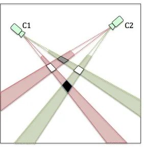
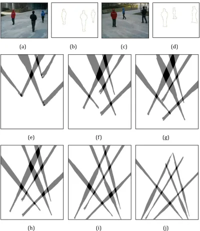
[image:19.595.242.383.453.598.2]Another problem with the homography approach is that the intersections of non-corresponding foreground regions can cause false-positive detections known as phantoms. Figure 1.3 is a schematic diagram to illustrate how non-corresponding foreground regions intersect and give rise to false positives. The warped foreground region in the top view is observed as the intersection of the ground-plane and the cones swept out by the silhouette of the underlying object. When the foreground regions for the same object are warped from multiple views to the top view, they will intersect at a location where the object touches the ground. However, if the warped foreground regions from different objects intersect in the top view, the intersection region will lead to a phantom detection. When homography mapping is based on a plane parallel to but higher than the ground plane, the projected foreground regions will move towards the cameras and additional phantoms may be generated. In Figure 1.3, the projected foregrounds from the two cameras intersect in four regions on plane p which is parallel to and off the ground plane. The white intersection regions are the locations of the two objects, whilst the black region that is intersected by the warped foreground regions of different objects is most likely to be a phantom. The grey region is an addition phantom.
Figure 1.3 A schematic diagram of the phantom occurrence in multi-view detection via homography mapping of foregrounds.
1.3
Organization of the Thesis
where the contour of each foreground region is approximated with a polygon and only the polygon vertices need to be transmitted and projected. Chapter 5 describes a geometrical approach to identify objects and phantom detections. Chapter 6 presents a combination method in which height matching and colour matching are applied successively to identify whether a foreground intersection region in the top view is due to same object or not. In this way, phantom detections can be identified. Conclusions and the future work are presented in chapter 7.
1.4
Contributions
The main research contributions of this thesis are highlighted as follows:
1) To accelerate the transmission and projection of the foreground information to a reference image, it is reasonable to focus on foreground regions. To warp the foreground regions in a camera view to the reference image, the contour of each foreground region is approximated by a polygon and the vertices of the polygon are projected onto the reference image using homography mapping. Then the foreground region is rebuilt by filling the polygon projected in the reference image. This approach greatly saves network bandwidth and accelerates the processing by avoiding the image-level homographic transformation.
2) To identify false-positive detections caused by the foreground intersections of non-corresponding objects in the top view, geometrical information of the foreground regions is utilised. As such, a height matching algorithm is proposed to match the intersection regions in the top view with the foreground regions in individual camera views to identify whether an intersection region is due to the same object.
2.
Literature Review
Although some good surveys on visual surveillance with multiple cameras have already been published [5-9], in this chapter a survey of the research in relation to this thesis is presented. It begins with a review of multi-camera visual surveillance systems and divides the existing systems into three categories according to the degrees of the information fusion from the multiple camera views. Then, the geometrical methods which are used to associate multiple cameras in the information fusion are reviewed. Since homography mapping is the method used in this thesis to associate individual camera views with a reference view, the related research using homography in multi-camera visual surveillance is discussed and then grouped according to the features used in the homography projection. Finally, the existing algorithms for the removal of false-positive detections are introduced.
2.1
A Review of Multi-Camera Visual Surveillance
As using multiple cameras in a visual surveillance system can provide a larger overall field of views and can reduce occlusions in the overlapping field of view, one of the key issues for visual surveillance with multiple cameras is how to utilize the information from the multiple cameras for the purpose of detection and tracking. The more information from the multiple cameras which can be used simultaneously, the more robust and accurate the system becomes. Depending on the degree of information fusion, the existing multi-camera surveillance systems can be categorized as low-degree information fusion, intermediate-degree information fusion and high-degree information fusion.
2.1.1
Low-
degree
Information Fusion
selected as the next optimal camera to track and monitor the object of interest and how to establish the correspondence of the objects between the cameras.
Cai and Aggarwal [10] proposed an algorithm, which starts tracking with a single camera view and switches to another camera when the system predicts that the current camera will no longer have a good view. The features extracted from the upper human bodies are used to build the object correspondence between cameras. The next camera should not only provide the best view but also have the least switching to continue tracking in that camera view.
In [11], the edges of the field of view of each camera, which can be seen in other cameras, are defined as field of view lines. The field of view lines are used to establish the correspondence of trajectories between cameras. The camera handoff is triggered when the object becomes too close to the edge of the camera’s field of view (EFOV). However, the authors did not give quantitative values of what is considered as too close to the EFOV and which camera is the most qualified camera to track the handoff object.
In these approaches, the detection and tracking are applied in separate cameras, and only one camera is actively working at a particular time stamp. Therefore, it fails to detect and track objects during dynamic occlusions as this is one of the problems with single-camera visual surveillance systems. Since there is very limited information exchange between the cameras, this camera switch approach is classed as a low-degree information fusion method.
2.1.2
Intermediate-
degree
Information Fusion
In addition to the tracking data, extracted features in individual camera views can be integrated into a reference view to obtain a global estimation. The extracted features include bounding boxes, centroids, principal axes and classification results. In [17], a motion model and an appearance model of each detected moving object are built. Then the moving objects are tracked using a joint probability data association filter in a single camera view. The bounding boxes of the moving objects are projected to a reference view according to the ground-plane homography to correct falsely detected bounding boxes and handle occlusions in the reference view. Du and Piater [18] use particle filters to track targets in the individual camera views and then project the principal axes of the targets onto the ground plane. After tracking the intersections of the principal axes using the particle filter on the ground plane, the tracking results are warped back into each camera view to improve the tracking in the individual camera views. Hu et al. [19] also project the extracted centre principal axes of each foreground object from the individual camera views to a top view according to the homography mapping for the ground plane. The foot point of each object in the top view is determined by the intersection of the axes projections from two camera views. The tracking is based on the foot point locations in the top view. In [20], global tracking is based on the intersections of the 3D lines, in which the centroids of the tracking targets are mapped from multiple views to 3D lines in terms of the world coordinates.
These methods are grouped into the intermediate-degree information fusion category of the multiview methods. Although these methods attempt to resolve dynamic occlusions through the integration of information from additional cameras as occlusions might not occur simultaneously in all the cameras viewing an object, they are still vulnerable to occlusion. The reason is that features are extracted from the individual camera views before fusion, and problems that arise in the detection and tracking with a single camera will affect the final fusion result.
2.1.3
High-
degree
Information Fusion
cameras are back-projected to yield points in the 3D world. These points are then projected onto the ground plane to generate the probability distribution map of the object locations. Berclaz, Fleuret and Fua [24, 25] divided the ground plane into grids to calculate the occupancy map in the ground plane. The probability that each sub-image corresponds to the average size of a person in each camera view is warped from each camera view to the top view for the ground-plane homographies independently.
The ground plane was later extended to a set of planes parallel to, but at some height off the ground plane to reduce false positives and missed detections [4]. In [26], a similar procedure was followed but the set of parallel planes are at the height of people’s heads. This method is able to handle highly crowded scenes because the feet of a pedestrian are more likely to be occluded in a crowd than the head. Their work achieves good results in moderately crowded scenes. The third category fully utilizes the visual cues from multiple cameras and has high-degree information fusion. This thesis will focus on the approaches in this category.
2.2
A Review of Multi-View Association
In multiple camera visual surveillance systems, one essential step is to establish the correspondence of objects between the cameras. In low-degree information fusion, feature matching is normally used to determine the correspondence among cameras and label the same target constantly when the camera is switched from one to another. In intermediate-degree and high-degree information fusions, the geometric constraints are used to associate different camera. The geometric constraints can be grouped into three categories: central projection based methods, epipolar line based methods and homography based methods.
2.2.1
Central Projections
world coordinate system, the mapping is an invertible one–to-many problem as that point corresponds to all points on that line. Since this leads to some of the classical problems in the establishment of correspondence across views, some features detected in the individual camera views are used to establish the correspondences. When feature points are transformed into the same world coordinate system, matching of the feature points is undertaken to indicate the corresponding feature points in the different views. The corresponding feature points in different views are projected at the same point in the world coordinates. In [35, 36], the centroids of the detected objects are used to establish the correspondences.
2.2.2
Epipolar Lines
The epipolar line is another constraint to associate objects across multiple camera views. When a point in one camera view is mapped to another camera view, all points lying on the epipolar line in the second view are potential candidates corresponding to the point in the first view. Since the epipolar constraint cannot build a unique correspondence between the two camera views, some feature matching approaches need to be added in the line search to help establish the correspondence across different camera views.
In [37], the epipolar geometry is improved by using detected faces, view volumes and colour cues. When the centroid of a face box in one view is projected to another view, the centroid of the face box in the new view, which has the least distance with the projected epipolar line, is considered as the corresponding centroid of the face box. Moreover, each view is divided into some non-overlapping volumes according to vertical features in the image. The matching of the view-volumes between the two cameras is embedded in the epipolar line method. The authors also used the hue and saturation values of each person as features to help establish the correspondence.
2.2.3
Planar Homographies
To solve the one–to-many problem in the central projection, a world plane is introduced [19, 38-40]. Using a common plane, when a point on that plane in the image is warped into the world coordinate system, its corresponding point in the world coordinate system lies on the intersection of that plane and the line passing through the centre of the pinhole camera. The common plane is a realistic assumption because most of the scenarios being monitored contain the ground plane, which make the imaging equation invertible.
In addition to using homography to link a camera view and the world coordinates on the ground plane, the projected world point can be projected into the same ground plane of a second image [41]. The correspondence between the points on the two image planes can be easily found. This property is referred to as the homography induced by that plane, which can be used to find correspondences across different camera views. A literature review on using homography to associate objects in multi-camera visual surveillance is provided in the next section.
2.3
A Review of Foreground Fusion with Homographies
Based on the features which are detected in individual camera views and are fused in the reference view to locate objects, homography mapping can be divided into three categories: pixel-based methods, line-based methods and region-based methods.
2.3.1
Foreground Pixel-based Methods
pixels above each foreground pixel on the vertical direction is calculated as a support of that foreground pixel and is normalized by a factor related to the perspective cross-ratio. The supports in each camera view are projected onto a virtual ground plane to determine the locations of pedestrians.
2.3.2
Foreground Line-based Methods
Foreground line-based methods use the principal axes of people as the feature in the homography mapping, as foreground pixels of a person are often symmetrically distributed along the principle axis. This can reduce the influence of motion segmentation errors. In [18, 19, 43], the authors projected the central vertical axis of each foreground object from individual camera views to a top view according to the homography of the ground plane. Then, the foot point of each pedestrian is determined as the intersection of the projected axes in the top view.
2.3.3
Foreground Region-based Methods
Arsic et al. [44] warped the contours of the detected foreground regions from each camera view to a virtual top view according to homographies. In [45], the silhouettes of the foreground in each camera view are applied in the multi-view moving object detection. Berclaz, Fleuret and Fua [24] divided the ground plane into grids to calculate an occupancy map in the ground plane. Each sub-image delimited by the grids is a rectangle that corresponds to the average size of a person in each camera view. The probability the each sub-image has a person is warped from the camera view to the top view by using the ground-plane homographies.
2.4
A Review of Colour Matching
As colour is a strong cue to identify moving objects, colour matching has been successfully applied in camera tracking and inter-camera tracking. For intra-camera tracking, objects from different frames within one intra-camera view are matched. For inter-camera tracking, it focuses on the association of the moving objects observed in different camera views.
measure, an explicit representation of colour is employed in the second method. Cheng et al. [47] built an appearance model of pedestrians based on the major colour spectrum histogram representation (MCSHR), where integrated MCSHR within 3-5 frames was applied to measure the similarity of moving objects in coping with small pose changes.
In Bowden and KaewTraKulPong [48], intersection of colour histograms in three colour spaces, RGB, HSL, and consensus – colour conversion of Munsell colour space (CCCM), were used for colour based object matching. In Gilbert and Bowdens [49], an incremental learning method was applied to model both the colour variations and posterior probability distributions of spatio-temporal links between cameras. In Park et al [50], each detected pedestrian was divided into three parts from the top to bottom, and the colours of the lower two parts in the HSV space were combined to generate a histogram for object matching. Porikli [51] proposed a distance metric and a non-parametric function to model colour distortion for pair-wise cameras and evaluate the inter-camera radiometric properties. Javed et al. [52] introduced an appearance model for each pedestrian by using colour histograms, in which the correspondence of pedestrians was established based on learning the usual change in colour of pedestrian during their moving between cameras, with the Bhattacharyya distance used to measure whether two observations were from the same object.
2.5
A Review of Phantom Removal
There are a number of algorithms which aim to remove these phantoms in foreground projection intersections. One solution is to avoid the generation of phantoms. Adding more cameras can provide a wider field of view and reduce the probability that a region cannot be visible in all views. Although additional cameras can reduce the sizes and number of phantoms, it is limited by the cost of the additional cameras [26]. Stering et al. [53] applied the idea of generalized Hough voting in the homography projection. Hough voting relates all foreground probabilities to a position on the ground plane and restrains the shadow generation. However, the authors stated that they cannot handle the case when objects cannot be visible in all camera views.
al. pointed out that phantoms appear from nowhere and checked their temporal coherence to test if a foreground intersection region existed in the previous frame. Khan and Shah [4] also filtered out the phantoms according to the temporal coherence. In Liem and Gavrila’s work, they assumed that phantoms are often unsteadily detected and checked the temporal coherence measured by a ‘hidden’ time rather than a single previous frame. If such a candidate cannot survive over the hidden time in tracking, then it is classified as a phantom. They also proposed that a new real object can only appear from the boundary of the overlapping field of views (FOVs); objects which are first detected in the middle of the overlapping FOVs are phantoms [54, 56].
The geometric approach is built on the comparison of features between phantoms and real objects. This approach can be further divided into two sub-classes: 3D space and 2D image methods, according to the types of geometric constraints that are used. The features applied in the geometric approach include heights and sizes. In the 3D space method, the comparison is in 3D space or in a virtual top view. Tong et al. [57] utilized foreground projection on multiple planes at different heights to removed phantoms. In [55], Yang et al. pointed out that the size of a phantom is often smaller than the minimum object size in the top view. However, this assumption is related to the height and viewing angle of the camera, and it does not work when a phantom region is covered by a real object in all camera views. Eshel and Moses [26] used the height information and assumed that the cameras are looking downwards. They found that if the viewing rays from two cameras intersect behind a true object, the phantoms are lower than the true object, taller phantoms occur when the rays intersect in front of true objects. By limiting the heights of real objects within an appropriate range, they could remove some phantoms.
foreground masks from all camera views are projected to a centroid plane to generate a occupancy likelihood map. The occupancy likelihood map is transformed to occupancy likelihood rays in the polar coordinate representation in each camera view, in which the origin of the polar coordinate is at the camera centre. The distance between the intersection region and the origin and the angle that each intersection region covered illustrate the death information and the size of that intersection region. Then, the depth information and covered angles are used to identify the occlusion relationship and remove phantoms.
2.6
Summary
3
HOMOGRAPHY ESTIMATION
In the previous chapter, methods to associate multiple camera views, which include the homography approach, were discussed. The objective of this chapter is to introduce the concepts of homography such as the homography transformation and homography estimation. Initially an introduction to projective geometry, the basics of a perspective camera such as the camera model, projections in homogeneous coordinate and camera calibration are discussed.
3.1
Camera Models and Calibration
Camera calibration is an important aspect in measuring the three-dimensional world. It provides a mechanism to build the relationship between a point in the 3D world and a point in the 2D image. It aims to estimate both the intrinsic parameters (such as focal length, principal points, skew coefficients and distortion coefficients) and extrinsic parameters (such as position of the camera centre and the orientation of the camera in world coordinates).
In camera calibration, the first step is to select a camera model and then to estimate parameters in that model. For many computer vision applications, the pinhole camera model has been widely used. It imagines a tiny hole on a virtual wall and assumes that the tiny hole only accepts the light rays passing through the tiny aperture in the centre and blocks other light rays. The central projection in the pinhole camera is depicted in Figure 3.1.
In Figure 3.1, there are four coordinate systems: the world coordinate system with subscript w, the camera coordinate system with subscript c, the image coordinate system with subscript i, and the pixel coordinate system with subscript s. A point in the world coordinate system needs three steps to be transformed into the pixel coordinate system. In the first step, the world coordinate system and the camera coordinate system are aligned by translating the origin of the world coordinate system to the origin of the camera coordinate system with a translation vector t and then by rotating the align axes with a 3×3 rotation matrix R which can be expressed by three elementary rotations. Since the translation vector t also contains three elements, the six parameters which define the orientations and 3D position of the camera are called extrinsic parameters in the camera calibration. Using the homogeneous coordinates, let be a point in the camera and be the corresponding point of in the 3D world, the relationship that maps to can be denoted as:
[
]
(3.1)[
𝑟
11𝑟
1𝑟
13𝑟
1𝑟
𝑟
3𝑟
31𝑟
3𝑟
33]
(3.2)[𝑡
𝑥𝑡
𝑦𝑡
𝑧]
(3.3)In the second step, the point is projected from the camera coordinate system to the image plane. The similar triangle relationships between these two coordinate systems are used because they have collinear axes in the Z direction. Let
be the corresponding point of in the image coordinate system, the relationship that maps to can be denoted by two equations:
𝑓
𝑓
(3.4)where f is the focal length of the lens, which is the distance between the principal point and the image plane.
where 𝑠𝑥 and 𝑠𝑦 are the sampling frequencies in the and axis, which are the number of pixels per unit length; 𝐶𝑥and 𝐶𝑦 are the principal point.
These two transformations which are a function of the camera can be described by a 3×3 intrinsic calibration matrix K:
𝐊 [
𝑓/𝑠
𝑥𝑠
𝐶
𝑥0
𝑓/𝑠
𝑦𝐶
𝑦0
0
]
(3.6)
where s in K is an effective scale factor which defines how far the axes are skewed in the direction of axis.
Then the full pinhole camera projection is generated. The relationship that maps to can be denoted as:
[
] [
𝑓/𝑠
𝑥𝑠
0
𝑓/𝑠
𝑦0
0
𝐶
𝑥0
𝐶
𝑦0
0
] [
𝑟
11𝑟
1𝑟
1𝑟
𝑟
𝑟
13 3𝑡
𝑡
𝑥𝑦𝑟
31𝑟
30
0
𝑟
330
𝑡
𝑧] [
]
(3.7)
The equation of the perspective projection is rewritten using a 3×4 projection matrix M:
𝐌
(3.8)Using a set of image points and the corresponding world coordinates, the extrinsic parameters and the intrinsic parameters in the perspective projection matrix M can be recovered and the camera calibrated. A simple approach uses a set of reference points involved the determination of transformation parameters to solve linear equations with known reference parameters [60]. Although it can provide an accurate and fast calibration result, the lens distortion cannot be handled and the reference points are hard to select in this approach.
Some method uses vanishing points to estimate the camera’s intrinsic and extrinsic parameters on the basis of geometric relationships such as parallelism and orthogonally in the scene [63]. The vanishing points are the converging points of parallel lines in a perspective projected image, which can be estimated from static scene structures, such as image edges which are either parallel or perpendicular in the world and landmarks [64] [65]. When architectural structures do not exist in the scene, the vanishing points can be estimated from object motion. In [66] [67], the authors detect the head and feet position of people walking during their leg-crossing phases. The line segments between heads and feet are used to estimate the camera’s intrinsic and extrinsic parameters. Zhang et al. [68] use the motion and appearance of moving objects and assumed camera height to estimate three vanishing points corresponding to three orthogonal directions in the 3D world coordinate system.
Since this research didn’t need very accurate calibration results, the simpler Tsai’s algorithm was used to calibrate the cameras and decide the relationship between a point in the 2D image and the same point in the 3D real world.
3.2
An Introduction to Homography
As discussed in chapter 2, planar homography is a special relationship, defined by a
transformation matrix H between a pair of captured images of the same plane with different cameras:
𝐇 [
ℎ
11ℎ
1ℎ
13ℎ
1ℎ
ℎ
3ℎ
31ℎ
3]
(3.9)
Let and be a pair of corresponding points on that plane in the two images. [ ] and [ ] are the homogeneous coordinates of those two points. They are associated by the homography matrix H:
′
≅ 𝐇
(3.10)where ≅ denotes that the homography is given up to an unknown scalar.
points in different images, though other features such as lines or conics in the individual images may be used [28] [69] [70]. These features are selected and matched manually or automatically from 2D images to compute the homography between two camera views or the homography between one camera view and the top view [71] [39]. Point based features are the most commonly used in estimating the homography, such as Harris corner points [72] and Scale-Invariant Feature Transform (SIFT) points [73]. In this thesis a set of manually selected corresponded points are used to estimate the homographies.
3.3.1
Point Correspondences
Given a set of corresponding points, the algorithms used to calculate the homography matrix can be divided into two classes: maximum likelihood estimation method and linear estimation method [74]. Given a pair of corresponding points and , equation (3.10) becomes two linear equations about H. The homography estimation is a process to calculate the solution of a set of linear equations about H. Since the homography matrix H is a homogeneous matrix, it only has 8 degrees of freedom or 8 unknowns which need to be solved. Then, if the number of correspondence point pairs N is 4 and no three points are collinear, the 8 unknowns of the homography matrix H can be solved uniquely with the 8 equations. If the number of correspondence point pairs N is more than 4, no exact H cannot be determined uniquely. Solving linear equations becomes the problem of optimal estimation of the parameters in H. Maximizing the likelihood and minimizing the algebraic distance are two methods to find the optimal parameters in H.
The Direct Linear Transform (DLT) algorithm [28] is the most widely used method to estimate the homography matrix H. Using the pair of correspondence points and , if the first row and the second row of equation (3.10) is divided by the third row respectively, equation (3.10) can be re-written as:
ℎ
11ℎ
1ℎ
13+ ℎ
31+ ℎ
3+
0
(3.11)ℎ
1ℎ
ℎ
3+ ℎ
31+ ℎ
3+
0
(3.12) Equations (3.11) and (3.12) can be further rearranged in a matrix form:where 𝐴 ( 0 0 0
0 0 0 ) 𝑖 ∈ [ 𝑁]
and 𝐡 ℎ11 ℎ1 ℎ13 ℎ 1 ℎ ℎ 3 ℎ31 ℎ3 .
A point matrix A is constructed by 𝑖 ∈ [ 𝑁] and then equation (3.13) can be rewritten as:
𝐀𝐡
(3.14)Equation (3.14) is over-determined and there is no solution in general. Choosing a suitable distance is considered and minimizing that distance can compute vector h. For the algebraic distance, the vector h can be computed by using Singular Value Decomposition (SVD) that minimizes the norm ‖𝐀𝐡‖ subject to ‖𝐡‖ [75]. In this research, the algebraic distance was selected because it has the least computation cost. Beside the algebraic distance, the geometric distance such as the total transfer error, the symmetric transfer error or the re-projection error for the corresponding point pairs and ′ 𝑖 ∈ [ 𝑁], can also be used.
3.3.2
Robust Estimation
When the input point correspondences are affected by inaccurate point correspondences or corrupted by false correspondences, to maintain the robustness of the homography estimation, these outlier correspondences should be removed. Random Sample Consensus (RANSAC) [76, 77]is a commonly used optimization method to remove outliers. The application of RANSAC for homography estimation works as follows:
1. A random sample of four correspondences is selected and a homography matrix H is computed from those four correspondences.
2. Each other correspondence is then classified as an inlier or outlier according to its concurrence with H.
3.3.3
Camera Calibration
The homography transformation is a special variation of the projective transformation. The point in the image without distortion and the point in the 3D world are limited on the ground plane. Therefore is 0 and the projection transformation from to becomes:
[
] [
𝑓/𝑠
𝑥𝑠
0
𝑓/𝑠
𝑦0
0
𝐶
𝑥0
𝐶
𝑦0
0
] [
𝑟
11𝑟
1𝑟
1𝑟
𝑟
𝑟
13 3𝑡
𝑡
𝑥𝑦𝑟
31𝑟
30
0
𝑟
330
𝑡
𝑧] [
0
]
(3.15)
Then, equation (3.15) can be rewritten as:
[
] [
𝑓/𝑠
𝑥𝑠
0
𝑓/𝑠
𝑦0
0
𝐶
𝑥𝐶
𝑦] [
𝑟
11𝑟
1𝑡
𝑥𝑟
1𝑟
𝑡
𝑦𝑟
31𝑟
3𝑡
𝑧] [
]
(3.16)
[
] [
ℎ
11ℎ
1ℎ
13ℎ
1ℎ
ℎ
3ℎ
31ℎ
3] [
]
(3.17)
The parameters recovered in the camera calibration can be used to determine the homography matrix for the ground plane.
3.4
Estimation of Multi-Plane Homographies
Homography mapping is not limited to the homography for the ground plane, and can be extended to a set of planes parallel to the ground plane and at some height. If the camera is calibrated, the multi-plane homographies can be calculated through the parameters recovered in the calibration process directly. After the homography matrix for the ground plane is estimated, the homography matrix for the planes parallel to and off the ground plane can be recovered from the perspective properties such as the vanishing point in the vertical direction [78] [4] or the cross-ratio of four collinear points [26]. The homography matrix can also be approximated according to the interpreted points [79].
3.4.1
Calibration
, where ℎ is removed. To represent the projection transformation matrix simply, M is rewritten as:
𝐌 [𝒎
𝒎
𝟐𝒎
𝟑𝒎
𝟒]
(3.18) According to equation (3.15), the ground-plane homography 𝐇 can be denoted as:𝐇
[𝒎
𝒎
𝟐𝒎
𝟒]
(3.19) Since the result, in which each element in the third column 𝒎𝟑 multiples the value ℎ in , is a constant value and the last element in the homogrenous vector is 1, according to the homography projection for plane p, the projection from point in the 3D world to point in the 2D image is:𝐇
[𝒎
𝒎
𝟐𝒎
𝟒+ ℎ 𝒎
𝟑]
(3.20) The homography of plane p can be represented as a combination of the homography for the ground plane and the third column of the projection matrix Mmultiplied by a given height h:
𝐇
𝐇
+ [ | ℎ 𝒎
𝟑]
(3.21)where [0] is a 2 zero matrix [78].
3.4.2
Vanishing Point
Under perspective projection, parallel lines in the 3D world space intersect at a point in the image. Therefore, one way to determine the perspective projection is to use vanishing points. In equation (3.18), the third column 𝒎𝟑 is defined as the vanishing point in the direction normal to the plane defined by 𝒎 and 𝒎𝟐 . When the camera is not calibrated, the homography for the plane at some height can be estimated by using the vanishing point with a scale factor [78]. Let be the vanishing point in the normal direction and 𝐇 be the homography between camera view a and ground plane g, the homography between camera view a and plane p parallel to plane g and at some height h is given as:
Let 𝐇 be the homography between camera view a and camera view b induced by ground plane g, the homography between the two camera views induced by plane p at a given height h is given as by [4]:
𝐇
(𝐇
+ [ | 𝛾
]) (𝐼
3 3+ 𝛾
[ | 𝛾
])
(3.23)
The main work focuses on the extraction of the vertical vanishing point. A static scene structures often contain many vertical parallel lines. These parallel lines in the scene are projected into the image. The projected lines in the image will ideally intersect at the vanishing point in the vertical direction. Therefore, the detection of the vertical vanishing point begins with the Canny edge detection [80] and the Hough transform [81]. Then a line detection algorithm is used to extract the dominant vertical lines. Finally, the intersection point of these vertical lines is calculated by minimizing the sum of its squared distances to all these lines.
3.5
Experiments and Analysis
Two video sequences were used to evaluate the performance of the algorithms proposed in this thesis. The first dataset is the PETS’2001 dataset which is standard image sequences for testing tracking and surveillance algorithms. The second dataset was captured at the thesis author’s campus. The ground-plane homography and homographies for planes parallel to and off the ground plane were calculated for each dataset.
3.5.1
Experimental Results of the PETS’2001
For the homography estimation, the top view image was selected as the reference image. To compute the homography matrix between each camera view and the top view, at least 4 pairs of correspondence points are needed. Although the world coordinates of the five landmark points in the dataset are provided, they cluster on one side of the image, which leads to inaccuracies in the homography estimation. As an alternative, a Google satellite image (http://maps.google.com/) for the same site was used as the top view image.
correspondences between feature points which are obtained automatically may include a significant amount of false matches. In this thesis, to calculate the homography for the ground plane, a set of landmark points were manually selected in the two camera views and the top view. The homography matrix is estimated as an offline process before the online moving object detection, which is a common practice in video surveillance systems.
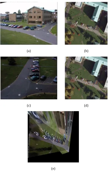
Figure 3.2 illustrates the process of the homography estimation by selecting a set of points in the top view. Figure 3.2 (a)- (d) shows the point set in two camera views and their corresponding top views. It should be noticed that (a) and (c) were not captured at the same time with the top view. Figure 3.2 (e) is a synthetic image generated by projecting and fusing the two camera views in the top view, in which the edges of the road are aligned.
3.5.2
Experimental Results of the Campus Dataset
(a) (b)
(c) (d)
[image:41.595.135.497.67.640.2](e)
(a) (b)
(c) (d)
(e)
[image:42.595.115.507.68.637.2]Table 3.1 The intrinsic parameters of the two cameras in campus dataset.
K (𝑚𝑚− ) 𝑓 (mm) 𝐶
𝑥 (pixels) 𝐶𝑦 (pixels)
Camera a 2. 7 0−4 22.76 320 240
Camera b .07 0−4 26.59 320 240
Table 3.2 The extrinsic parameters of the two cameras in campus dataset.
𝑡𝑥 𝑡𝑦 𝑡𝑧
Camera a 98.0 68.4 .47 03
Camera b 6.4 0 32.28 . 03
(a) The translation vector t.
𝑟11 𝑟1 𝑟13 𝑟 1 𝑟 𝑟 3 𝑟31 𝑟3 𝑟33
Camera a 8.7 0−1 4.86 0−1 .80 0− 7.54 0− .72 0−1 9.82 0−1 4.80 0−1 8.56 0−1 .87 0−1
Camera b 8. 7 0−1 5.4 0−1 6.59 0− .64 0−1 . 5 0−1 9.77 0−1 5.2 0−1 8.29 0−1 2.02 0−1
(b) The rotation matrix R.
Figure 3.4 Fusion of the projected background images in the top view.
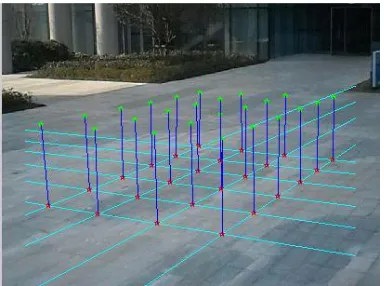
Then, using equation (3.21), the homography for a plane parallel to and at the height of h can be calculated. In Figure 3.5, the selected points in Figure 3.3(e) are warped back from the top view to camera view a according to the homography for a plane at the height of 1 meter. The warped back points are the green points in Figure 3.5, which are connected with their corresponding landmark points on the ground plane.
Figure 3.5 Warped back points corresponding to the selected points in Figure 3.3(e).
[image:44.595.217.409.483.626.2]4
MOVING OBJECT DETECTION
WITH REAL-TIME FUSION
In the previous chapter, the algorithms to calculate homographies for the ground plane and the multiple planes parallel to the ground plane at different heights were introduced. In high-degree information fusion, using the calculated homography matrices, the foreground image, which is extracted from each of the multiple camera views, can be mapped to a reference view.
In traditional homography mapping, each pixel in a camera view needs to be projected into the top view according to the homography for a plane. Since this mapping is a pixelwise projection, the number of pixels to project is determined by the resolution of the camera view. To avoid perspective openings or holes which are generated during the mapping from the camera view to the top view, each pixel in the top view is warped back to the camera view according to the inverse homography transformation. If a warped back pixel is located in a foreground region in the camera view, the original pixel in the reference view is labelled as a foreground pixel. The number of pixels in the homography mapping is decided by the resolution of the top view, which is usually higher than that of the camera view because the top view normally covers a larger area.
Due to the high resolution of the top view, the pixelwise homography mapping is very time consuming and needs high bandwidth, which makes it hard to apply the homography approach in real-time applications. This brings about a challenging requirement on the bandwidth of multi-camera networks. If the foreground detection and multiview foreground fusion are carried out by different computers, the pixelwise homographic transformations at image level, for multiple cameras and multiple parallel planes, are more time consuming and thus prevent any low cost real-time implementation.