Aid Volatility, Policy and Development

This is a repository copy of Aid Volatility, Policy and Development.

White Rose Research Online URL for this paper:

http://eprints.whiterose.ac.uk/9972/

Monograph:

Hudson, J. and Mosley, P. (2007) Aid Volatility, Policy and Development. Working Paper.

Department of Economics, University of Sheffield ISSN 1749-8368

Sheffield Economic Research Paper Series 2007015

[email protected]

https://eprints.whiterose.ac.uk/

Reuse

Unless indicated otherwise, fulltext items are protected by copyright with all rights reserved. The copyright

exception in section 29 of the Copyright, Designs and Patents Act 1988 allows the making of a single copy

solely for the purpose of non-commercial research or private study within the limits of fair dealing. The

publisher or other rights-holder may allow further reproduction and re-use of this version - refer to the White

Rose Research Online record for this item. Where records identify the publisher as the copyright holder,

users can verify any specific terms of use on the publisher’s website.

Takedown

If you consider content in White Rose Research Online to be in breach of UK law, please notify us by

Sheffield Economic Research Paper Series

SERP Number: 2007015

ISSN 1749-8368

John Hudson* and Paul Mosley

*

Aid Volatility, Policy and Development

.

October 2007

* Department of Economics

University of Sheffield

9 Mappin Street

Sheffield

S1 4DT

United Kingdom

Abstract

We build on Bulir and Hamann's analysis of aid volatility (2003, 2005), showing that

the conclusions reached depend on the dataset used. Their argument that the

poorest countries have the highest volatility appears not to be correct. The impact of

volatility on growth is negative overall, but differs between positive and negative

volatility. The mix between ‘responsive’ components of aid, e.g. programme aid, and

‘proactive’ components, e.g. technical assistance, is important. Finally, we conclude

that measures which increase trust between donor and recipient, and reductions in

the degree of donor ‘oligopoly’, reduce aid volatility without obviously reducing its

effectiveness.

Keywords: aid volatility, disasters, trust, upside and downside volatility.

Co Author: University of Bath:

[email protected]

Introduction

The copious and in many ways inconclusive literature on aid effectiveness does now contain some elements of consensus, one of which is that the qualities or characteristics which define the aid relationship may be important in determining effectiveness: for example geographical distribution, distribution by aid type and the pattern of aid flows through time. Our focus in this paper is on the last of these, and in particular on the volatility, or instability, of the aid flow. A priori it looks probable that volatility of revenue inflows, a high proportion of which are aid in the case of the poorest countries, may cause harm in a number of ways which are likely to be damaging for investment and for development. Firstly, volatile aid inflows result in variability of expenditure and thus in a proliferation of half-complete projects, thus lowering their rate of return. Second, volatile inflows especially in the form of technical assistance and consultancy result in high staff turnover, discontinuity of relationships within the aid donor-recipient community and, as a consequence of the resulting low levels of social capital, limited opportunities for learning on the part of both parties (Lele and Goldsmith 1989 for the case of aid to the agricultural sector). Third, the unstable expenditure disbursements resulting from volatile inflows create an unpredictable policy environment, which deters both domestic and foreign investment (Rodrik 1990) and, more than this, makes macro-economic management of any sort difficult (Heller et al 2006): neither the level of expenditure nor the budget deficit, which are fundamental elements in macro-policy, can be predicted in any of the very poor countries (including most in Africa) where aid, which finances most development and some recurrent expenditure, is itself unstable. These problems may get worse if, as has been advocated, aid to Africa and other poorer countries is doubled over the next five years in an attempt to reach the Millennium Development Goals (Foster and Killick 2006).

A plausible working hypothesis, therefore, is that volatility is bad for aid effectiveness, and that the effectiveness of the aid flow into a particular country will vary inversely, other things being equal, with its volatility. Exploratory confirmation of this idea is provided by the empirical studies of Lensink and Morrissey (2000) and Mosley and Suleiman (2004); the most comprehensive critique, however, is that put forward by the IMF economists Ales Bulir and Javier Hamann(2003, 2005). Bulir and Hamann (B-H) argue that the volatility of aid is;

greater than that of government revenue;

increasing over time;

and pro-cyclical (in other words, aid flows are inversely correlated with the level of government expenditures in any particular year).

Our paper examines both the dimensions of the aid volatility problem, as examined by Bulir and Hamann, and their consequences. We begin (section 2) by examining the B-H conclusions, looking at both theoretical issues and empirical evidence. We then (section 3) move beyond B-H to decompose volatility by region and policy instrument and the extent and impact of donor co-ordination and concentration, all of which appear to exert an influence on volatility. In section 4, we examine the impact of volatility on indices of well-being such as economic growth, and discover that that impact is asymmetric as between ‘upside’ and ‘downside’ volatility. Finally (section 5) we conclude the paper with a discussion of possible policy responses. Key in these is the building of trust between donors and aid recipients. We also present a model schema which might form the basis for future empirical work.

2. Examining Bulir & Hamann

Our sample of 76 countries and period of analysis, 1975 to 2003, is identical to that used by Bulir and Hamann in their paper in this symposium (Bulir and Hamann 2006) and, like them, we compare for these countries the relative volatility (coefficient of variation) of aid and domestically-generated revenue. Our methodology is also identical to theirs, namely the measurement of the residuals from a Hodrick-Prescott filter, with two exceptions. First, by contrast with Bulir and Hamann, we define all variables as a proportion of their mean value for the whole estimation period, multiplied by 100 – hence, in our analysis, the average value of each variable is 1001. Secondly, when measuring the relative volatility of aid and domestically-generated revenue we prefer to measure the ratios of median, not mean revenue

1

in each country2. To assess the sensitivity of volatility measures to the unit of measurement, we measure volatility in domestic currency, in US dollars and as the ratio of aid to GDP.

In our application of the Hodrick-Prescott filter, we used a value for lambda of seven3. In our analysis, the ratio of aid to government revenue volatility ( ) is in excess of one for almost all countries, and indeed our estimate of the number of countries for which is less than one (10) is smaller than theirs (16). The reason for this, we would argue, is that by normalising around an arbitrary mean of 100 we have removed the scale factor from the variance, i.e. the tendency for low ratios of aid or expenditure to GDP to have low variances. Thus a country such as Algeria, which does not receive much aid relative to government revenue, is likely to have a much lower aid variance simply because this reflects variations around a smaller number.

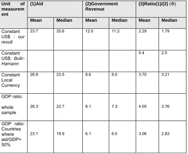
Table 1 summarizes the results for each of the variables examined by Bulir and Hamann. As may be seen from the table, the measurement of aid volatility is more or less invariant with respect to the choice of units; but this is not the case for government revenue. Least volatility is evident for government revenue expressed as a ratio of GDP, slightly more when expressed in terms of the local currency, and substantially more when government revenue is expressed in US$. Indeed in US$ volatility is approximately 60% greater than when defined in terms of the GDP ratio. The mean is of course sensitive to outliers and perhaps a better indication of the situation for the representative country is given by the median. Again we observe a similar pattern of results, although measures of volatility based on the median are lower than those based on the mean. In taking a ratio, volatility will reflect both elements of the ratio. Government spending is likely to be positively correlated with GDP and this will tend to reduce the variance of a ratio in a manner which is less likely for the aid to GDP ratio. When government revenue is expressed in terms of US$ the variability of the exchange rate impacts on the measure of aid volatility, increasing it unless there is a negative correlation between the two variables. Exchange rate variability impacts on aid volatility whichever measure is used provided aid budgets are basically determined in terms of donor currencies. Hence the ‘fairest’ comparison is in terms of US$ where both variables are impacted upon by exchange rate variability and volatility relates to aid or government expenditure rather than these variables relative to GDP.

Table 1 also shows relative volatilities ( ). The smallest relative volatility is that using the median for standard deviations based on both measures in constant US$ where aid is 179 percent more volatile than government revenue. When we move to the mean the figure is 226 percent. The greatest difference is when the measures are expressed as a ratio of GDP with the arithmetic mean showing aid to be 405 percent more volatile than government revenue.4/ The comparison is most favourable to aid, on our measures, when both variables are expressed in terms of US$ and least favourable when expressed as a ratio to GDP. This has similarities to B-H’s conclusion (Bulir and Hamann, 2006) that falls when they use per capita measures rather than GDP ratio measures, i.e. is greater when based on the GDP ratio. Our analysis has provided an insight as to why this should be the case.

B-H take the average as defined by the mean and also the median. We argue that the latter is preferable in this case because of the properties of a ratio. Given two countries, one with government volatility twice that of aid volatility and the other with the opposite scenario, relative volatility defined as the ratio of aid to government revenue volatility will be 0.5 and 2.0 respectively with a mean value of 1.25, misleadingly implying that volatility is greater for aid than for government revenue.

3

The Hodrick-Prescott filter or H-P filter is an algorithm for choosing smoothed values for a time series. A larger value of lambda makes the resulting series smoother with less high-frequency noise. A lower value tends to follow the original series more closely. For more details see Bulir and Hamann (2003).

Table 1: Summary Measures of Volatility: all countries in sample

(volatility expressed as standard deviation of variable indicated)

(1)Aid (2)Government

Revenue

(3)Ratio(1)/(2) ( )

Unit of measurem ent

Mean Median Mean Median Mean Median

Constant US$ : our result

23.7 20.6 12.0 11.2 2.29 1.79

Constant US$: Bulir-Hamann

5.4 2.5

Constant Local Currency

26.8 23.5 8.6 8.0 3.70 3.21

GDP ratio:

whole sample

26.3 22.7 8.1 7.3 4.05 3.76

GDP ratio: Countries where aid/GDP> 50%

23.1 19.9 6.1 6.0 3.06 2.83

Sample: 76 countries for period 1975-2003, as specified by Bulir and Hamann(2003). Source for all data is OECD World Development Indicators. Bulir-Hamann result in row 2 is taken from Bulir and Hamann(2006), table 2.

In their original paper B-H found that volatility is highest in the countries which are most aid-dependent, which are generally the poorest and most vulnerable . They argue that ‘the relative volatility of aid grows with aid dependence: the average value of increases from 3.94 to 7.42 as the sample is narrowed down to the most aid-dependent countries’(Bulir and Hamann, 2003: 69). However, in their latest paper, Bulir and Hamann ( 2006: 15 ) find that the pattern is more complex, and that both countries which are little dependent on aid and countries which are heavily dependent on aid display high aid volatility relative to government revenue. We confirm that we can find no evidence for highly aid dependent countries to have higher volatility (a higher value of ). Table 1 presents results for those countries with an to-government revenue ratio greater than 50 percent , and finds that the most aid-dependent countries actually have lower volatility than the sample as a whole. Indeed, volatility declines as the aid-revenue ratio increases: if we regress relative volatility, measured in US$, on the mean aid government revenue ratio (AID/GREV), we get:

= 2.53 – 0.55AID/GREV (1)

(13.11) (3.16)

OLS estimation; R2 = 0.09, n=47.

indicates that relative volatility declines as the aid to government revenue ratio rises. Our belief is that once scale factors are taken out of the calculations, as is achieved by our practice of normalising the data, it is impossible to find any evidence to support the view of higher volatility in the very high aid-to-GDP countries5. It is notable that when Bulir and Hamann move from expressing variables in absolute values in the original paper (2003) to expressing them in natural logs in their second paper (2006), scale factors are taken out of the calculation by a similar route to our procedure of normalising the data, and as a consequence the result that aid-dependent countries are more volatile disappears.

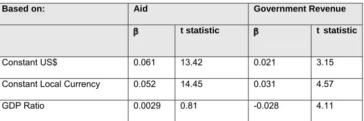
Secondly, we explore the issue of whether volatility has been increasing over time. To analyse this we regress the square of the residual obtained from the Hodrick-Prescott filter (ujt2) on a trend (TREND).

This procedure is similar to that used to model the variance in a GARCH or ARCH model (Engle, 1982). Of course in any one time period, for any country, the error term can be close to or far from zero. But if there is a trend in volatility over time it will be reflected in a significant coefficient on the trend in this regression. We take the square of the residual because residuals can be positive or negative and we are interested in their absolute size and hence absolute distance from zero, rather than whether they are positive or negative. The best fit was obtained when a loglinear equation was used. If volatility has been increasing (decreasing) then on average the squared error term will also be increasing (decreasing) and the coefficient on the trend variable will be significantly positive (negative). The results for both aid and government revenue are shown in table 2.

Table 2: Volatility Through Time

Based on: Aid Government Revenue

β t statistic β t statistic

Constant US$ 0.061 13.42 0.021 3.15

Constant Local Currency 0.052 14.45 0.031 4.57

GDP Ratio 0.0029 0.81 -0.028 4.11

Coefficient of β in regression log(ujt2) = α + βTRENDt, where ujt is the residual for the j’th

country in period t from the application of the Hodrick Prescott filter on normalized aid or government revenue.

The first point to note is that in all three sets of regressions aid volatility is increasing by more than government revenue volatility. Hence when measured in normalized constant US$ the trend on aid is almost three times greater than that on government revenue. This clearly implies that, as B-H concluded, is increasing over time. It is interesting to note the differences in the trends when different measures are used. When we move from US$ to local currency the trend on aid is less than twice that on government revenue. In this case the trend on aid has declined and that on government revenue increased. The trend will reflect the different movements in the components of the variance, which in this case are core revenue volatility plus exchange rate volatility. The decline in β for government

revenue as we move from local currency to US$ suggests that the impact of exchange rate volatility relative to core revenue volatility has been declining over time. This is also consistent with the increase in β for aid as we move from local currency to US$.6/ There is one significantly negative trend factor in these regressions, that for government revenue as a ratio of GDP. This tentatively suggests that budgetary or other changes have resulted in government revenue tracking GDP more closely over

On theoretical grounds this is exactly what we would expect. As aid increases it becomes an increasingly greater component of government revenue and hence in terms of their statistical moments the two variables should show some convergence.

6/ 5_{The impact of the exchange rate between local currency and US$ affects government revenue as we}

time.7/ In all three sets of regressions, the gap between β in the aid and government revenue regressions is of the order of 0.02 to 0.04 and this is a reflection in the difference in the underlying trends in core aid and government revenue volatility.8/

The conclusion so far, therefore, is that although the volatility of aid is indeed a serious and increasing problem for developing countries, there is no evidence that it impacts hardest on the poorest and most vulnerable. What is important is to understand in more detail what causes it, what harm it does, and how that harm can be mitigated. That is the task attempted in the following two sections.

3. Beyond Bulir & Hamann

In this section we test two explanatory hypotheses: that aid volatility is determined by the composition of the aid budget between aid instruments and by the level of donor concentration within individual countries. Both hypotheses have relevance for any prescription to reduce the harmful effects of volatility.

Aid Volatility by Region and Policy Instrument

First, we speculate that the volatility of aid may vary according to its type. The hypothesis from which we begin is that aid which is essentially reactive – in response to an emergency, or an economic crisis, or a collapse of commodity prices – is far more likely to be subjected to sudden upwards or downwards movements, and thus to be volatile, than aid which is proactive, consisting of a planned programme of activities on which disbursement is reasonably steady and predictable.

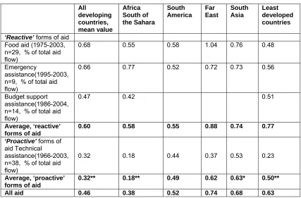
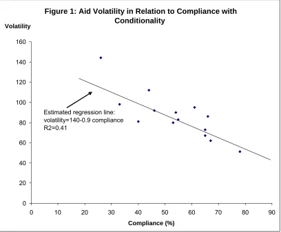
In Table 3, we disaggregate the OECD aid flow, for the period 1975-2003, into its reactive and proactive components, and discover that the level of volatility on reactive aid activities - food aid, emergency aid9 and programme aid in particular – is indeed higher than on proactive aid activities, in particular technical assistance. Technical assistance is the form of aid which is arguably least linked to short-term factors10 and it is interesting to note that in residual terms it displays a much greater degree of stability than the other categories of aid, whereas categories of aid which are more need-responsive, such as food aid and budget support aid, are more volatile than the average. Especially in the case of budget support aid, volatility frequently arises from a cut-off of funds following a recipient country’s failure to comply with performance criteria attached to an (IMF) stand-by agreement or (World Bank) adjustment loan: the volatility of programme aid flows is tightly correlated, across our sample, with slippage on conditions as illustrated by Figure 111. This appears, on the surface, to support Bulir and Hamann’s recommendation that ‘a higher degree of compliance with conditions attached to aid is likely to lead to a smoother path of [aid] disbursements’ (2003, p.82). However, there is substantial variation from case to case: disbursement is, for various reasons including the bargaining power of the recipient, not always cut off when conditions are not complied with (for example Mosley, Harrigan and Toye 1995, Mosley and Suleiman 2005), which carries the implication that failing to punish poor performance may reduce short-term volatility but impair its credibility and thus its ability to improve policy over the long short-term. Another fundamental factor causing variations in volatility between recipients at constant levels of compliance is

Low values of revenue volatility may be seen as a consequence of evidence of fiscal rigidity, rather than as a success. They are consistent with evidence that developing countries, especially poorer ones, have limited ability to ‘target’ the revenue/GDP ratio, i.e. tax revenue may vary because of random shocks but governments have been unable to achieve increases in tax/GDP ratios. One implication is that it is very difficult to adjust revenue to compensate for aid volatility (especially shortfalls)

8/ 7_{Again one has to emphasize that this relative impact would change if we were to use the square root of}

ujt2.This is similar to basing the measures of volatility on the standard deviation rather than the variance. 9

One of the highest volatility levels of all is experienced by Ethiopia, which also has one of the highest levels of emergency and food aid on account of its high incidence of drought and conflict.

10

Note however that (as pointed out by a referee) not all technical assistance expenditure is delivered through the recipient budget; some (eg some consultancy and training fees) is not even spent in the recipient but in the donor country!

11

the level of underlying trust between donor and recipient which has evolved through the course of programme aid negotiations12.This illustrates a much broader point: the volatility of aid is often an

Table 3 Aid Volatility Disaggregated by Region and Policy Instrument

(standard deviation of net ODA for region and period stated)

All developing

countries, mean value

Africa South of the Sahara

South America

Far East

South Asia

Least developed countries

‘Reactive’ forms of aid Food aid (1975-2003, n=29, % of total aid flow)

0.68 0.55 0.58 1.04 0.76 0.48

Emergency

assistance(1995-2003, n=9, % of total aid flow)

0.66 0.77 0.52 0.72 0.73 0.56

Budget support assistance(1986-2004, n=14, % of total aid flow)

0.47 0.42 0.51

Average, ‘reactive’ forms of aid

0.60 0.58 0.55 0.88 0.74 0.77

‘Proactive’ forms of aid Technical

assistance(1966-2003, n=38, % of total aid flow)

0.32 0.18 0.44 0.37 0.53 0.23

Average, ‘proactive’ forms of aid

0.32** 0.18** 0.49 0.62 0.63* 0.50**

All aid 0.46 0.38 0.52 0.74 0.68 0.63

Sources: World Bank World Development Indicators; OECD Geographical Distribution of Financial Flows to Less Developed Countries. ** denotes difference between sample means (for ‘proactive’ and ‘reactive’ forms of aid) significant at 1% level, * denotes difference significant at 5% level.

inescapable by-product of characteristics of aid frequently seen as positive, in particular its ability to respond to a crisis or exert beneficial policy leverage over a recipient country. A reduction of volatility due to this cause, therefore, may have an opportunity cost in terms of other potential benefits of aid not achieved. This theme is further taken up in the last two sections, where a key distinction is made between positive and negative volatility. The former represents sudden shortfalls in aid and the latter increases or surges in

aid. Within this context, food, emergency and humanitarian aid are all

sources of positive volatility, corresponding to the Lensink and Morrissey (2000) conjecture

that aid volatility in part captures responses to adverse shocks to the economy, and the

adverse impact on growth is due to these shocks, not the aid volatility. On the other hand,

interruptions to programme aid or budget support aid, for example, are sources of negative

volatility which may in themselves impact adversely on growth.

Figure 1: Aid Volatility in Relation to Compliance with

Conditionality

Volatility

160

140

120

Note: Volatility is defined here as the coefficient of variation of World bank/IMF programme assistance. From left to right the countries are: Zimbabwe, Sierra Leone, Kenya, Nigeria, Cote D’Ivoire, Tanzania, Malawi, Zambia, Senegal, Mozambique, Ethiopia, Lesotho, Ghana and Uganda.

Volatility and Donor Concentration

We now consider aid volatility by donor. We consider whether a larger or smaller number of donors leads to a lower level of volatility. We assume two donors (x and y), The combined volatility of aid, ( ) is given by

= xx + yy + 2 xy (2)

Let us assume that xx= yy and compare this with the case when the same aid budget as provided by

the two donors is provided by a single donor. Let us divide this aid budget into two identical halves each with a variance of xx, then by definition

= xx + xx + 2 xx = 4 xx (3)

The difference between this and the former case lies in the difference between xx and xy. Only in the

case where the two countries’ aid budgets are perfectly correlated will we get xy = xx, failing this xy < xx. This then gives us the intuitively plausible result that aid volatility will generally be less the greater

0 20 40 60 80 100

0 10 20 30 40 50 60 70 80 90

Compliance (%)

the number of donors. Hence a multiplicity of donors will, we surmise, tend to reduce aid volatility, even if the aid flows between donors are positively correlated, provided that correlation is less than 1.

To test this intuition, which is similar to that of Fielding and Mavrotas (2005), data was taken from the DAC statistics database. The list of recipient countries, chosen on the basis of aid receipts in 2000, are shown in table 4. The selection of donors was chosen to provide: (i) a picture ‘in the round’: thus all DAC donors, all donors, the EU and the G7,are included; (ii) information on leading country donors and (iii) also information on the behaviour of some smaller donors. In analysing the data the procedure was followed of regressing aid per se, on a constant, trend, trend squared and trend cubed. Aid was expressed in absolute values, not logs, as sometimes aid is zero and sometimes even negative and it would be arbitrary to exclude these values from the data. Thus if aid from donor i to recipient j is in successive years, 100, 150, 0, 125, the zero is a valid observation. Nor was the Hodrick-Prescott filter used. B-H note, and we also found, that the results were similar to when filters based on time trends were used. The H-P filter makes more demands on the data and we did not wish to reduce the number of observations when calculating the cross-correlations. In addition, the data is very volatile for some countries and is subject to severe spikes. The technique we use is less sensitive to individual outliers than the H-P filter.

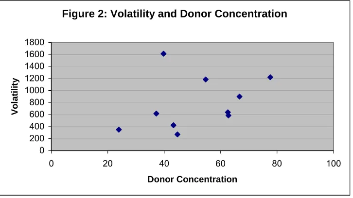
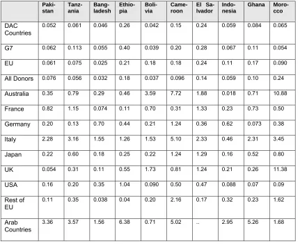
The greatest volatility for all DAC donors is experienced by Ethiopia, El Salvador and Cameroon. The periodic famines in Ethiopia partially explain the high variance of aid to that country. There is a tendency for the countries with high two-donor concentration ratios, i.e. the share of aid provided by the two biggest donors, to have relatively high volatility. This is shown most clearly in Figure 2, where the volatility and concentration ratios are based on all (DAC) countries. The correlation is not perfect, but we would not expect it to be in the light of factors including the mix of aid types previously mentioned. We can see that volatility tends to be greater for individual donor countries rather than for a collectivity of countries, which again illustrates the point that the sum of the whole is less volatile than its individual parts.

Figure 2: Volatility and Donor Concentration

0 200 400 600 800 1000 1200 1400 1600 1800

0 20 40 60 80 100

Donor Concentration

Vola

tilit

Table 4: Volatility in specific countries, by aid donor

Paki-stan

Tanz-ania

Bang-ladesh

Ethio-pia

Boli-via

Came-roon

El Sa-lvador

Indo-nesia

Ghana

Moro-cco

DAC Countries

0.052 0.061 0.046 0.26 0.042 0.15 0.24 0.059 0.084 0.065

G7 0.062 0.113 0.055 0.40 0.039 0.20 0.28 0.067 0.11 0.054

EU 0.061 0.075 0.025 0.21 0.18 0.18 0.24 0.11 0.17 0.090

All Donors 0.076 0.056 0.032 0.18 0.037 0.096 0.14 0.059 0.10 0.24

Australia 0.35 0.79 0.29 0.46 3.59 7.72 1.88 0.018 0.71 10.88

France 0.82 1.15 0.074 0.11 0.70 0.31 1.33 0.23 0.73 0.50

Germany 0.20 0.13 0.70 0.44 0.21 1.24 0.36 0.62 0.073 0.38

Italy 2.28 3.16 1.55 1.26 1.53 5.10 2.33 0.46 2.31 3.45

Japan 0.22 0.60 0.18 0.25 0.22 1.24 1.29 0.16 0.52 0.80

UK 0.054 0.31 0.11 0.55 1.73 0.81 1.24 0.21 0.26 11.38

USA 0.16 0.20 0.35 1.04 0.090 0.50 0.47 0.088 0.07 0.09

Rest of EU

0.11 0.35 0.038 0.04 0.20 2.16 0.17 0.32 0.23 1.62

Arab Countries

12

Table 5: Substantial Donor Correlations

Recipient Negative Positive Recipient Negative Positive

Pakistan 12 14 El Salvador 8 19

Tanzania 10 12 Indonesia 14 15

Bangladesh 4 17 Ghana 7 14

Ethiopia 4 36 Morocco 9 16

Bolivia 7 18

Cameroon 14 11 Total 89 172

Note: the figures give the number of recipient pairs with an absolute correlation of 0.2 or greater

We now turn to the correlations between the residuals for different countries. In Table 5 we show the number of ‘large’ positive or negative correlations for each recipient ; the former dominate. This should be interpreted as, e.g., for Pakistan there were 12 large negative correlations between donors and 14 large positive ones, where large is to be interpreted as an absolute correlation in excess of 0.20. Thus there is, on balance, a tendency for donors to be positively co-ordinated in giving aid to specific countries, which suggests that they tend to respond to common signals and are impacted upon by common factors such as a global economic cycle.

4. Consequences of Aid Volatility

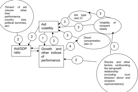
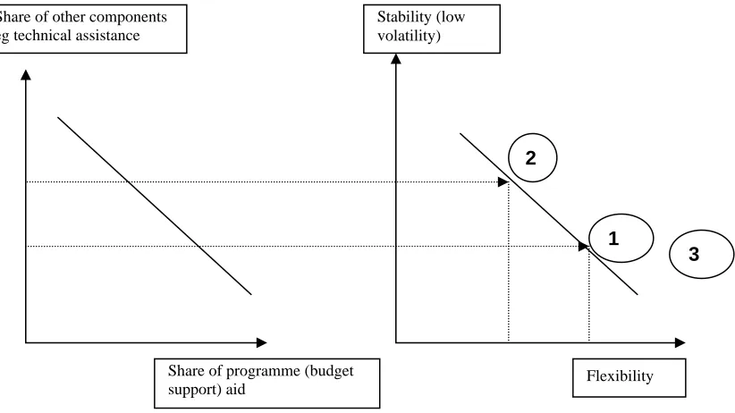
Figure 3. Aid volatility and growth in a model of simultaneous causation

(circled numbers represent equation numbers, see Appendix)

Aid

volatility

Growth and

other indices

of

performance

Aid type (sec.3)

Donor concentration (sec.3)

Volatility of recipient needs

3

3

3

3

3

4

2

3

Shocks and other factors confounding the aid-growth

relationship

(including trust

between donor and recipient

representatives)

‘Drivers’ of aid volume other than

performance,

country size, political dummies, etc)

1

2

2

13

We now shift the focus from the causes to the consequences of aid volatility. A priori, it is not obvious that Bulir and Hamann’s claim (2005, p1) that ‘the positive impact of aid has been frustrated by the lack of reliability in aid flows’, is necessarily true. The study by Lensink and Morrissey (2000) finds that the impact of aid on growth is significantly positive only when the volatility of aid is controlled for, and in Mosley and Suleiman (2005), aid volatility has a negative influence on headcount poverty, in both cases across a period from the early 1980s to the early 2000s. However, these findings are by-products of larger investigations into aid effectiveness, and do not embody any ideas on the causes of volatility. We here incorporate the hypotheses on determinants of volatility presented in the previous section into an extremely simple model of the simultaneous determination of volatility and growth.

This model (figure 3) spells out some of the likely causes and effects of aid volatility. There are several feedbacks from the consequences to the causes, requiring the application of simultaneous-equation methods.The logic behind the model is the following. Aid volatility is likely to be higher:

The more the aid flow is concentrated in the hands of one or a few donors, as discussed in the previous section, on the grounds that if this is the case any fluctuations in the flow of one aid donor cannot be offset by compensating variations in the flows of other donors;

The more the donor’s aid flow is concentrated in forms of aid which are innately exposed to fluctuation. Some forms of aid need to be volatile in order to work: for example flows of a ‘compensatory’ nature, such as food aid, and conditional programme aid, which to be effective need to be cut off in the event that the recipient does not comply with the terms of the policy contract. As argued in the previous section (see also Fielding and Mavrotas 2005) the larger the share of the budget which the donor puts into these ‘intrinsically volatile’ components, the greater the volatility of aid will be;

The greater the volatility of the recipient’s needs over the time period under examination, since aid is a response to the recipient’s predicament. Thus recipients exposed to shocks are more likely to experience volatile aid flows.

These factors are combined into an equation for volatility (equation 3) which then impacts on growth (equation 1). This growth equation embodies the simultaneous linkage between aid and development indicators such as growth and poverty (equation 1), which current research suggests to be reasonably robust and positive (Hansen and Tarp 2001, Mosley, Hudson and Verschoor 2004) together with a standard set of ‘new growth theory’ variables. The model, finally, shows a feedback loop from recipient poverty to the donor concentration ratio (equation 4), on the grounds that there is more likelihood cet. par. of a wide spread of donors in countries which are very poor and thus have a strong developmental case for aid.

Within the context of this model, we seek to isolate the influence of volatility on growth. Our hypothesis here is that this influence is not homogeneous, but depends largely on the root causes of volatility itself. If the root cause of volatility is an emergency, to which the response is an aid surge, then this response may be seen as the intended resolution of, rather than the cause of, the fundamental problem: in which case, providing the response is effective, volatility, or the element of responsiveness in aid, is beneficial. If, however, aid volatility is due to exogenous factors, - an unexpected decline due to an emergency elsewhere13 or a downturn in the global economic cycle, then aid volatility is more likely to be damaging. In general, we expect an asymmetry of impact between upside and downside volatility: a priori, it is improbable that fluctuations of aid levels above the mean, which ease resource constraints, will have the same short-run impact as fluctuations below the mean, which are often responsible for them14.

We now estimate the impact of volatility on growth within the context of the model of Figure 3. We take the residuals previously obtained from the Hodrick-Prescott filter relating to the growth rate (Table 1 above). These residuals were then divided into positive and negative terms, i.e. ‘positive aid residuals’ takes a value equal to the aid residual when this is positive and otherwise zero. We feel this to be important on the grounds that, as argued above, positive volatility constitutes a different kind of shock from negative, such that the two kinds of deviation from the mean are unlikely to be symmetric in effect. One key difference between our work

13

The war in Iraq is a good illustration of an ‘emergency elsewhere’ which has made the aid budgets of several donors (especially the US and UK) to countries outside the Middle East unexpectedly volatile.

14

14

and much previous literature on aid effectiveness is that we will be using panel data based on annual data, rather than cross section data based on, e.g., ten yearly periods. This is necessary if we are to distinguish between the impacts of positive and negative volatility, but also permits the use of explanatory variables not often included in this type of analysis. In particular we include, as shocks likely to influence the response of the economy to aid volatility, the growth of OECD countries as an influence on developing countries’ exports, and a measure of the incidence of disasters or emergencies, such as major floods, earthquakes, famines or droughts. In addition we examine whether there is any crowding out effects of disasters on other aid recipients, i.e. whether a large disaster or disasters in some countries reduces aid flows to others. We will also be using ‘good policy’ variables, such as low inflation, as specified in the original Dollar and Burnside paper15.

Within a system such as Figure 3, it is traditional to estimate the growth equation with aid being treated as an endogenous variable. As Delgado et al. (2004) argue, this may not be necessary when using annual data, but is more likely when using grouped data. We will be testing for endogeneity and use a simultaneous equation technique, but feel the greater problem is one of serially correlated error terms. The structure of the aid equation will include data on disasters, a time trend and the growth of OECD countries. The time trend will, in part, capture trends in donor budgets. The growth rate of OECD countries is also included for this reason. Other variables will include recipient lagged gdp per capita to capture the hypothesis, along with the time trend, that low income countries have the greater potential for growth via catching up. We will also include various country fixed effects as used in other studies. The data on disasters comes from EM-DAT: The OFDA/CRED International Disaster Database16. In order for a disaster to be entered into the database at least one of the following criteria has to be fulfilled: (i) 10 or more people reported killed, (ii) 100 people reported affected, (iii) a call for international assistance or (iv) a declaration of a state of emergency. Disasters include floods, earthquakes, epidemics, droughts, famines, windstorms, etc. There are three measures of data available, (i) the number killed, (ii) the number affected and (iii) the value of the damage done. We feel that the number killed may not give an appropriate indication of the impact on the economy or aid flows – a large number can be killed in a relatively contained disaster with little overall impact. The value of the damage done is a better measure of impact but this measure is still being developed and hence we use the number of people affected and restrict this to where the number affected is above 10% of the population. The variable we use is the percentage of the population affected. The number of such disasters has been steadily increasing, which may be part of the reason for the increasing time trend in aid volatility reported in table 2: in 1960-64 there were just two disasters classifiable in this way, whereas in the period 1998-2001 the number had risen to 77. In part this reflects the impact of climate change and there has not been such a great increase, for example, in earthquakes. Clearly this subject needs further research and the measure further refinement but we feel that this does represent a potentially important area of new research.

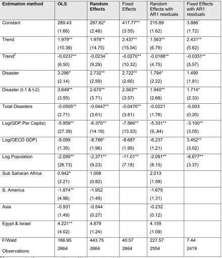
Table 6 reports the results of estimating the aid equation (equation 1 in figure 3). The countries included in the analysis in the rest of this paper now extend beyond those used in the B-H paper to encompass all those where data is available from the World Bank data base. The dependent variable is aid expressed as a ratio of GDP in periods t and t-1. The Breusch and Pagan Lagrangian multiplier test suggests that random effects is superior to OLS, whilst the data makes the Hausmann test to distinguish between fixed and random effects inapplicable. The results, in line with other studies, indicate an inverse relationship between aid and both GDP per capita and population. Also in line with other studies is the significance of the dummy variable for Egypt and Israel. The coefficients on the time trend and the time trend squared suggest that aid (measured as percentage of GDP) has been increasing over time but at a decreasing rate. This reflects a number of influences. Firstly ‘the generosity’ of donor budgets, but secondly ‘the target’ against which GDP per capita is compared. This target should at least be non-declining over time and the fact that the combined effect of the time trend was to peak at about the beginning of the new millennium suggests that donor generosity has also peaked at some time in the sample period.The coefficients on disasters and lagged disasters suggests that these are an important factor in determining aid, and as discussed in the context of Table 3, its volatility: they are a classic illustration of ‘reactive’ aid. The coefficients suggest that the greater response comes not in the year of the disaster, but in the following years17. In addition the coefficient on total disasters over the last three years18 is significant in almost all the regressions suggesting a crowding out effect. This suggests that an

15

The CPIA index of good policy is not really possible to use as it is not available on an annual basis over the period we are covering. For similar reasons variables such as ethnic fractionalisation and the proportion of land in the tropics are of little added value as they will become redundant within the context of a fixed effects estimation.

16

http://www.em-dat.net/index.htm

17

In this case the two following years. The fact that these were significant does not necessarily indicate that the effect lasts just for these two additional years, merely that with limited data this is what we were abel to establish.

18

15

emergency fund to be allocated specifically for disasters would not only allow a speedy response – our results tentatively suggest a somewhat delayed response – to a specific disaster, but reduce the adverse impact on other aid recipient countries. The results also suggest substantial residual auto-correlation over time, which is why we report the results of AR estimations.The evidence of autocorrelation suggests that it takes time for aid flows to adjust to changed realities, and when aid is either above or below trend levels, it tends to stay so for a long time. There are many reasons why this might be so, but one, briefly discussed in our earlier analysis of budget support aid is trust between donor and recipient. Trust can keep aid flows above what they apparently ‘should be’, but a lack of trust can have the reverse effect. This is a possibility we turn to later.

Table 6: Regressions of Residuals on Aid/GDP Ratio

(Figure 3, equation 2)

Estimation method OLS Random

Effects Fixed Effects Random Effects with AR1 residuals Fixed Effects with AR1 residuals Constant 289.43 (1.66) 287.62* (2.48) 417.77** (3.55) 215.89 (1.62) 3.886* (1.72) Trend 1.979** (10.38) 1.978** (14.75) 2.437** (15.04) 1.563** (6.79) 2.431** (5.62)

Trend2 -0.0237** (6.50) -0.0234** (9.29) -0.0270** (10.32) -0.0188** (4.75) -0.0351** (5.57) Disaster 3.296* (2.14) 2.732** (2.59) 2.722** (2.60) 1.794* (2.22) 1.490 (1.81)

Disaster (t-1 & t-2) 3.649**

(3.55) 2.675** (3.71) 2.563** (3.57) 1.940** (2.68) 1.714* (2.33)

Total Disasters -0.0505**

(2.71) -0.0447** (3.61) -0.0470** (3.81) -0.0221 (1.76) -0.003 (0.20)

Log(GDP Per Capita) -5.959**

(27.39) -6.370** (14.19) -7.566** (13.53) -5.331** (9,.84) -3.100** (3.05)

Log(OECD GDP) -9.099 (1.35) -8.766* (1.96) -8.687 (1.95) -6.237 (1.21) 3.452** (3.02)

Log Population -2.095** (26.73) -2.371** (9.23) -11.01** (7.18) -2.091** (8.15) -6.677** (3.37)

Sub Saharan Africa 0.942*

(2.21)

1.008

(0.82)

2.013

(1.59)

S. America -1.874**

(4.96) -1.952 (1.49) -1.675 (1.31) Asia -0.931 (1.49) -0.544 (0.27) -0.232 (0.12)

Egypt & Israel 4.221** (4.02) 4.879 (1.24) 4.159 (1.09) F/Wald Observations 166.95 2664 443.75 2664 40.57 2664 227.57 2554 7.44 2419

16

Table 7 presents estimates of the central relationship in Figure 3, the impact of volatility and other variables on growth (relationship (2))19. The first column reports results estimated with OLS. Aid is significantly positive at the 5% level. However, this is somewhat neutralized by the impact of aid volatility. The results suggest that both positive and negative volatility reduce growth20, and in the results we have for the most part combined the two together. However, this does not mean that the two are symmetric in their impact. When we look at lagged volatility there is a substantial difference in their impact. Negative volatility is insignificant, whilst positive volatility is significant and reduces some of the previous harmful impact on aid. If the problems raised by positive volatility are linked with absorptive capacity as is suggested in the literature, these results suggest that these are to an extent short term only and are reversed in subsequent periods. But with negative or downside volatility there is no such reprieve. Unlike the aid regressions the disaster variable is only significant in the current time period. Of the other variables, growth in the OECD countries is transmitted to the developing countries in the current period. There is also a catch-up effect by which growth in developing countries tends to be greater in the poorest countries and the regional dummy variables are also of varying significance. Finally lagged inflation, representing a good policy environment as in the original Burnside and Dollar (2000) paper, is significant with the anticipated negative sign. In the remaining columns we used standard fixed and random effects and then correcting for autocorrelation. Given that we are dealing with time series data within a panel data context we felt this to be a likely problem and the results suggest that indeed there is autocorrelation. The results are relatively consistent, apart from the time trend and lagged GDP which are substantially different when using fixed effects. In addition inflation is generally not significant. In all of these aid tends to be significant at the 1% level. The test statistics suggest that fixed effects is superior to random effects. As indicated earlier the possibility that aid is endogenous is perhaps unlikely. We test for this using the augmented version of the Durbin-Wu-Hausmann (DWH) test developed by Davidson and MacKinnon (1993). The relevant F statistic is 3.13 and is insignificant at the 5% level, hence endogeneity appears unlikely to be a problem, although in the last two columns we nonetheless report the results of instrumental variable estimation, where aid in its pure and interactive forms are instrumented as indicated in Table 6. The results are largely unchanged from the previous regressions. The level of significance in all of these regressions, as indicated by the F or Wald statistic, is not high. This is inevitable given that we are dealing with very noisy series. Nonetheless the large sample sizes help in extracting information from the data as reflected in the variables which are mostly significant at the 1% level. The Breusch and Pagan Lagrangian multiplier test suggests that random effects is superior to OLS, whilst the Hausmann test indicates fixed effects is preferable to random effects, although the key parameter estimates relating to volatility differ relatively little between the two techniques.

In Table 8, the results obtained with the approach taken in this paper, of differentiating the effect of positive and negative residuals, are contrasted with the approaches taken by previous authors who treat volatility as a unitary or ‘symmetric’ variable. Studies of aid volatility impact vary according to their welfare criterion selected as dependent variable: Mosley and Suleiman (2004) used the poverty headcount, and Lensink and Morrissey (2000) the investment rate. Both find a negative impact of aid volatility on the criterion variable chosen. In other regressions Lensink and Morrissey also show, for all developing countries and the SSA sub-sample, that aid has a positive effect on growth if the regression includes ‘aid uncertainty’, i.e. unanticipated volatility rather than total volatility but omits investment. Thus the beneficial effect of aid is via investment rather than via efficiency in addition to investment. In this study, growth of GDP is the dependent variable. Variables are also defined in different ways, e.g. in some cases logs are used in others not. Hence it is best to compare the significance rather than the size of coefficients. However, our results confirm the negative impact of aid volatility, but when we differentiate between the lagged impact of such volatility we find that the damage done by positive volatility is to an extent reversed in subsequent periods.

Panel cointegration techniques have not been used to test for stationarity in part because of the gaps in some of the data series.

20

17

Table 7: Regressions of Residuals on Growth

Dependent Variable: Annual Growth of GDP

(Figure 3, equation 1)

Estimation method

OLS Random

Effects Fixed Effects Random Effects AR1 Fixed Effects AR1 Random Effects IV Fixed Effects IV

Constant 7.092** (5.94) 10.16** (6.27) 45.447** (12.43) 8.362** (4.90) 38.63 ** (10.12) 8.794** (4.43) 36.273** (8.38)

Trend -0.0264 (1.57) -0.00434 (0.24) 0.293** (9.33) -0.0156 (0.77) 0.244 (6.76) -0.0089 (0.47) 0.254** (7.84)

Disaster -2.772* (2.48) -3.550** (3.21) -2.564* (2.31) -2.419* (2.15) -2.107 (1.83) -3.829 (3.41) -4.741 (4.19)

Aid GDP ratio 0.0380* (2.38) 0.0665** (3.29) 0.164** (5.83) 0.0664** (3.15) 0.143 (4.56) 0.122** (2.93) 0.433** (4.84)

Inflationt-1 -0.00036*

(2.45) -0.00021 (1.47) -0.00016 (1.12) -0.00015 (1.00) -0.0001 (0.47) -0.00025* (1.71) -0.00036 (2.39)

Volatility -0.101** (4.58) -0.105** (4.68) -0.148** (5.83) -0.0993** (4.50) -0.125** (5.20) -0.158** (3.80) -0.187** (4.49) Positive Volatility t-1 0.0636** (3.24) 0.0687** (3.55) 0.0433* (2.26) 0.0635** (3.34) 0.0529** (2.75) 0.0669** (2.67) -0.0402 (1.10) Negative Volatility t-1 0.0147 (0.20) 0.0473 (0.66) -0.0127 (0.18) 0.0382 (0.54) 0.0120 (1.83) 0.0704 (1.02) 0.0414 (0.60)

World Growth 0.289** (4.06) 0.293** (4.26) 0.209** (3.11) 0.317** (4.41) 0.231** (3.20) 0.303** (4.36) 0.257** (3.65) Sub Saharan Africa -1.741** (5.59) -2.401** (5.22) -2.140** (4.56) -2.579** (5.32)

S. America -1.243** (4.49) -1.172** (2.72) -1.142** (2.63) -1.163** (2.61)

Asia -0.883* (1.91) 0.659 (0.95) 0.826 (1.17) 0.749 (1.04)

Log(GDPPCt-2) -0.353*

(2.26) -0.844** (3.82) -6.796** (11.93) -0.591** (2.59) -5.711 (8.48) -0.690** (2.65) -5.708** (9.21) F/Wald Observations 10.40* 2666 118.7 2666 29.34 2554 99.47 2554 17.91 2419 115.4W 2664 30.27 2664

**_/* _{denotes significance at the 1% and 5% levels.}

18

Table 8 : Impacts of Volatility on Growth: Overview

Estimation method Panel data, fixed effects 2SLS combined with AR(1) forecasting equation

3SLS

Dependent variable Growth of GDP Investment Poverty headcount Investigator This study

(Table 7, column 4)

Lensink and Morrissey, 2000 Mosley and Suleiman, 200421/ Regression

coefficients on independent variables:

Whole sample Africa

only Constant 8.632** (4.90) 15.16** (8.42) 4.26 (1.82) -42.3** (4.64) Aid as % GDP 0.064**

3.15) 0.22* (1.92) 0.23** (2.51) 0.034 (1.61) Disaster measure -2.419*

(2.15) Aid volatility measure:

‘Aid uncertainty’22/

Volatility as in this paper

CV of aid

-0.0993** (4.50) -0.77** (2.81) -0.47 (1.29) 0.175* (2.45) Lagged Volatility: Positive: Negative: 0.0635** (3.34) Not significant

World growth 0.317** (4.41) GDP per capita

(logged in our study)

-0.591** (2.59) -0.0003** (4.13) 2.23* (4.18)

GDP/cap, squared -0.18**

(5.12) Time trend -0.100**

(8.18)

Trade openness 0.059** (3.63)

0.142** (3.62)

0.095 (1.16) Inflation (lagged one

period) -0.00015 (1.00) Ratio of money/GDP 0.114 (1.74) 0.246** (3.24)

R2 0.36 0.57 0.61

Wald Statistic 99.47

Number of obs 2554 88 43 663

Sources: as stated in row 3 of table. Figures in parentheses are Student’s t-statistics: ** indicates significance of a coefficient at the 1% level and * indicates significance at the 5% level.

21/ _{Other variables in regression: government expenditure, shares of agriculture, education and basic social}

services in government expenditure, food crop yields, total crop production, regional dummies, country fixed effects.

22/ _{Deviation from ‘anticipated aid’, as derived from extrapolation of a time trend in aid to the recipient}

country under examination.

19

5. Conclusion

We now seek to summarise the major conclusions so far:

First, the volatility of overseas aid is severe (in relation to the volatility of domestic revenue) and increasing over time; but there is no observable tendency for volatility to be most severe in the poorest and most vulnerable countries.

Second, three of the major determinants of aid volatility appear to be the volatility of recipient needs, the mix of aid between ‘reactive’ and ‘proactive’ types of aid, and the degree of donor oligopoly. Aid volatility increases as the recipient’s country’s natural and political environment become more volatile, as the share of ‘reactive’ forms of aid within the budget increases, and as the number of donors diminishes.

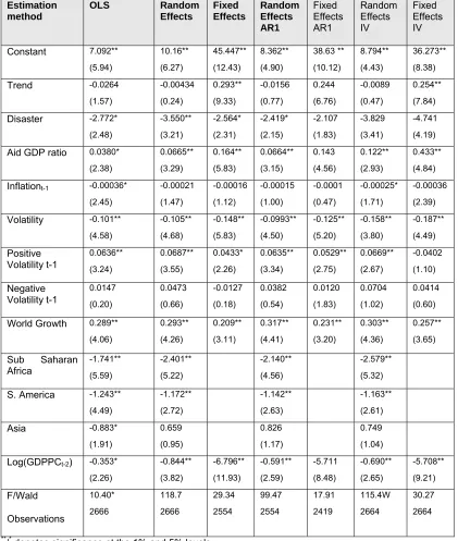
Third, volatility as a whole reduces growth given the level of aid; but not in a uniform way. The initial impact of both upside and downside volatility is to reduce the impact of aid. But subsequently some of this negative impact is reversed but only for upside volatility. With downside volatility there is no such impact. This may reflect problems of absorptive capacity being short term only. Upside volatility may also be reacting to emergencies and reflects an element of flexibility inherent in ‘reactive’ forms of aid. The high incidence of this type of aid, is therefore in principle an asset rather than a liability. Even negative volatility might feasibility have longer term beneficial impacts, in persuading recipients to move towards policy reform, which are not apparent within the relatively short time horizon we are looking at. The question as we visualise it is therefore not to try and reduce the volatility of aid to zero, but rather to reduce those elements in volatility which cause harm: or, to take the approach extensively developed in this symposium by Eifert and Gelb (2006) to seek to move the trade-off , represented on figure 4, between stability and flexibility23:

Figure 4. The trade-off between flexibility and stability of overseas aid

In the diagram an increase in the relative share of budget support aid leads to a reduction in stability and an increase in flexibility. For a mathematical derivation of the trade-off, see equation (6) of the Appendix.

Stability (low volatility) Share of other components

eg technical assistance

2

1

3

Share of programme (budget

support) aid Flexibility

20

We can visualise four ways24 in which donors might seek to shift, or at worst move along, this trade-off in the interests of development, achieving an increase in the stability of aid flows (reduction in volatility) without sacrifice :

Changes in the mix of aid instruments. From the evidence of Table 3, measures which increase the ratio of ‘proactive’ to ‘reactive’ aid (eg increases in the share of technical assistance expenditure) will reduce volatility25. If this is done by means of increases in the aid level, so that the resources available for reactive aid functions do not diminish, flexibility will not be sacrificed and the trade-off can be moved outwards.

Mechanisms for increasing trust between aid donors and recipients. Within the category of ‘reactive’ aid modalities and in particular programme (budget support) aid, it is possible to achieve greater stability by achieving a greater climate of trust between donors and recipients, in which donors do not react by withdrawing aid (and thereby making it unstable) each time a performance criterion is breached, but maintain aid levels stable as long as there is agreement on ‘underlying principles’: Poverty Reduction Strategy Papers are intended to be an instrument for helping to achieve stability of disbursements by means of a focus on essentials. In material terms, this increases the resources available to the aid recipient. There is evidence of a trust-building process of this kind occurring between the early 1990s and the early 2000s in the economies of (more or less in chronological sequence) Uganda, Ghana, Ethiopia, Mozambique and Tanzania, with a recent reversal in Ethiopia. Where such a trust-induced improvement takes place, there is a Pareto improvement, and it is possible to speak of a movement in the trade-off (a movement from 1 to 3 on figure 4). As illustrated by Figure 1, one way of achieving this is compliance with donors’ conditionality. However, it has been a development of the last ten years in particular to show that other trust-building mechanisms, less weighted towards the donor, exist. Including the opening of donor resident missions in recipient countries, the development of home-grown pro-poor expenditure plans designed by recipients rather than donor agencies , effective control of corruption and initiative taking within policy dialogue (Mosley and Suleiman 2006). An important priority for future research is to understand what are effective trust-building mechanisms going beyond the above, and what has been their ability to influence the volatility of aid in different environments.

Increases in the degree of donor competition. As illustrated by Tables 4 and 5 above, aid is more volatile in cases when the number of donors is small. An increase in competitiveness, in which many donors are supplying a particular recipient country, appears to limit the volatility of aid to that country: luckily, this appears to be easiest to achieve in the poorest countries, and we can observe evidence of its occurrence in Ethiopia, Tanzania, Rwanda, Uganda and Mozambique. Our finding that volatility is not particularly high in the poorest countries (table 1) appears to be connected to this.

Institutional options such as an ‘aid buffer-stock fund’. In their contribution to this symposium Eifert and Gelb (2006) have made a rigorous attempt to simulate the shape of the tradeoff between reducing volatility and other goals using simulation methods. They visualise aid as being stabilised by means of a simple insurance mechanism: a buffer stock equal to three months’ import cover. They simulate the impact of providing such a buffer stock, and conclude that ’losses (from lack of flexibility) are modest in most cases, and become very small with a ‘flexible commitment’ rule where changes only kick in where governments’ performance ratings rise or fall substantially’ (Eifert and Gelb 2006: 230). At the moment, such simulations have to be based on sparse knowledge of the impacts of volatility in different settings; however, elaborations of the initial results presented here, based on a broader range of data, may gradually ease these problems.

These four suggested approaches are supplementary to the idea of greater coordination between aid donors, which has been attempted over a long period without great success in a number of countries; also, this idea partly clashes with the idea of greater competition between aid donors, recommended

25

But see the caveat at footnote 9 above.

21

References

Adam, Chris, and Jan Willem Gunning,2002, ‘Redesigning the aid contract: donors’use of performance indicators in Uganda’, World Development, vol. 30, pp. 2045-2056.

Arellano, Cristina, Ales Bulir, Timothy Lane and Leslie Lipschitz(2006) ‘The dynamic implications of foreign aid and its variability’, paper presented at UNU-WIDER conference on Aid: principles, policies and performance, Helsinki, 16-17 June.

Bulir, A., and J. Hamann (2003) ‘Aid volatility: an empirical assessment’, IMF Staff Papers, vol 50:1,pp 64-89.

Bulir, A., and J. Hamann (2005) ‘Volatility of development aid: from the frying pan into the fire?’ Washington DC: IMF, paper submitted to this symposium.

Collier, P. (1997) ‘The failure of conditionality’ in C. Gwin and J. Nelson(eds.) Perspectives on aid and development, Washington DC: Overseas Development Council.

Collier, P. and D. Dollar(2001) ‘Can the world cut poverty in half? How policy reform and effective aid can meet international development goals’, World Development, vol. 29, pp. 1787-1802.

Collier P. and D. Dollar(2002) ‘Aid allocation and poverty reduction’ European Economic Review, vol 46, pp. 1475-1500.

Dalgaard CJ, H. Hansen H and F. Tarp (2004) On the empirics of foreign aid and growth Economic Journal, vol. 114, pp. F191-F216.

Engle, R. (1982) ‘Autoregressive Conditional Heteroscedasticity with Estimates of United Kingdom Inflation’, Econometrica, vol 50, pp 987-1008.

Fielding, D. and G.Mavrotas (2005) ‘On the volatility of foreign aid: further evidence’, unpublished paper, WIDER, Helsinki.

Foster, M. and T.Killick(2006) ‘What would doubling aid do for macroeconomic management in Africa?’, paper presented at UNU-WIDER conference on Aid; Principles, policies and performance, Helsinki, 16-17 June.

Gelb A. and B. Eifert(2005) ‘Improving the dynamics of aid: towards more predictable budget support’. Paper submitted to this symposium.

Gillman M. and A. Nakov (2004) ‘A Granger causality of the inflation-growth mirror in accession countries’, Economics of Transition, vol 12, pp. 653-681.

Harrigan, Jane, 2003,’U-turns and full circles; two decades of agricultural reform in Malawi 1981-2000’,

World Development, vol. 31, pp. 847-863.

Heller, Peter, et al. 2006, ‘Managing fiscal policy in low income countries: how to reconcile a scaling-up of aid flows and debt relief with macroeconomic stability’, paper presented at UNU-WIDER conference, Helsinki, 16-17 June.

Leandro, Jose, Hartwig Schafer and Gaspar Frontini(1999) ‘Towards a more effective conditionality: an operational framework’, World Development, vol. 27, pp.

Lele, Uma and Arthur Goldsmith(1989), ‘The development of national agricultural research capacity: India’s experience with the Rockefeller Foundation and its significance for Africa’, Economic Development and Cultural Change, vol. ,pp. 305-343.

Lensink, R. and O. Morrissey(2000), ‘Aid instability as a measure of uncertainty and the positive impact of aid on growth’, Journal of Development Studies, vol. 36,pp. 31-49.

Mosley, Paul, Jane Harrigan and John Toye(1995) Aid and Power, second edition. London: Routledge.

Mosley, Paul (2003) ‘The World Bank and the reconstruction of the ‘social safety net’ in Russia and eastern Europe’, unpublished conference paper, Yale University. Forthcoming, Yale University Press.

22

Mosley, Paul, John Hudson and Arjan Verschoor(2004) ‘Aid, poverty reduction and the new conditionality’, Economic Journal, vol 104(June 2004) 217-244.

Mosley, Paul, and Suleiman Abrar (2004) ‘Aid, agriculture and poverty’, paper presented to HWWA conference on The Political Economy of Aid, Hamburg, 10-12 December. Forthcoming, Review of Development Economics.

Mosley, Paul, and Suleiman Abrar(2005) ‘Trust, conditionality and aid-effectiveness’. Paper presented to Budget Support Forum, Cape Town, 5/6 June. Now published in S. Koeberle, Z. Stavreski and G. Verheyen,

Pearson, K. (1979). ‘On the Scientific Measure of Variability’, Natural Science, vol 11, pp 115-118.

Ramey, Gary and Valerie A. Ramey(1995) ‘Cross-country evidence on the link between volatility and growth’, American Economic Review, vol. 85, 1138-1151.

Rodrik D.(1990) ‘Are structural adjustment programmes effective? (check title) World Development

Schultz, Theodore W. (1960) ‘Value of US farm surpluses to less developed countries’ Review of Economics and Statistics.

Van der Vaart, R (1979). ‘Statistical Study of Variances’, in (W H Kruskal and J M Tanur, eds.)

International Encyclopedia of Statistics, pp 1215-1226, Free Press, New York.

World Bank (2000) World Development Report: Attacking Poverty. Washington DC.

23

Appendix

Volatility within an Aid-Effectiveness Model

This appendix sets out in algebraic form the relationships comprising the model of Figure 3 above (page 14). The model is in essence an aggregate ‘new growth theory’ production function with endogenous aid flows (equations 1 and 2) of the kind which has been used to estimate aid and growth regressions for many years (e.g. Mosley, Hudson and Horrell 1987; Hansen and Tarp 2001; Mosley, Hudson and Verschoor 2004). The novelty here is that aid volatility appears as an additional independent variable in the production function, and is then modelled (equation 3), on the basis of our findings in section 2 of this paper, as a function of the structure of aid flows and the volatility of the recipient country’s needs.

In order to focus attention on the effects of aid volatility, the specification of the model is kept extremely simple, and there is no discussion of other factors affecting aid effectiveness (e.g. resource allocation in the public sector) on which much of the effectiveness literature has concentrated. The model is written out in aggregative form, without country subscripts. There are four fundamental relationships in the model:

(1)The aggregate production function

( Y/Y) = f1(A,- (A), F; K, L,H, P) (1)

in which Y = recipient country income, Y = change in recipient country income, A = aid as a proportion of recipient GDP; (A) = volatility (standard deviation) of aid disbursements; K= physical capital stock, H= human capital stock, L= labour force, P= vector of policy variables influencing aid effectiveness. The expected sign of the coefficient on aid volatility, (A), is negative, and on all other independent variables is positive.

This is the ‘new growth theory’ relationship estimated in table 7. In our formulation, growth is determined not only by aid and the standard ‘new growth theory’ factors of production, but also by

attributes of the aid flow, including aid volatility (A) and flexibility F (the increment to aid effectiveness which results from being able to adjust aid flows to the circumstances of the economy and the behaviour of policy makers).

.

(2)Determinants of aid flows

A = f2 ( Y, S, C, P) (2)

in which S = a measure of the incidence of shocks on the recipient economy, C= a measure of country size, P = a measure of political factors affecting aid allocations including political and military ties

between the recipient and specific donors.

This is a standard instrumenting equation for aid flows; estimates of the equation are presented in Table 6. For the subsequent argument of this paper it is important that any volatility in the indicators of ‘recipient need’, Y (recipient income) and S(shocks to recipient income) will be automatically converted through (2) into volatility in what we have called the ‘reactive’ component of aid flows.

(3) Determinants of volatility( )

(A) = 1 + 2 (Ar/Ap) + 3DCR + 4 ( Y/Y) (3)

We now seek to explain the determinants of volatility in aid flows. As shown in section 2 above, volatility is a positive function of the ratio of ‘reactive’ to ‘proactive’ components of aid(Ar/Ap) (since when aid

reacts to an emergency or other trigger, that makes it depart from its mean value, or become volatile) and a negative function of the donor concentration ratio DCR (the number of donors in the country, which may taken as an indication of the dependence of the country on individual donors, or inversely as an indicator of the degree of monopoly of those donors). In addition, volatility in aid responds to the volatility of the growth of recipient national income: any emergency or economic crisis in the recipient national economy will increase is vulnerability and create a need for aid, and to the extent donors respond to this, the volatility of aid itself will increase.