A General Equation Based on Entropy Generation Minimization to Optimize Plate Fin Heat Sink

Article

A General Equation Based on Entropy Generation

Minimization to Optimize Plate Fin Heat Sink

Hossain Nemati

Department of Mechanics, Marvdasht Branch, Islamic Azad University, Marvdasht, Iran E-mail: [email protected]

Abstract. In the present study, a new method based on entropy generation minimization

was proposed to optimize plate fin heat sink. It is clear that the design of a heat sink is not straightforward and needs some secondary equations. Therefore, in the present study, dimensionless forms of equations were presented first and the effect of each dimensionless group on the entropy generation rate was studied deeply. Finally, a semi-analytical equation was proposed to relate dimensionless thickness to dimensionless fin height and Bi number as well. Interestingly, since no restricting assumption was made during derivation, this equation can be used for both natural and forced convection. Moreover, this equation is based on dimensionless parameters, so it is not limited to some specific geometries or working conditions. At the end, six examples showed benefits and ease of use of this equation. A fan curve was also used in optimizing a heat sink which is more realistic than using a specified free stream velocity.

Keywords: Entropy generation minimization, natural convection, forced convection, heat sink.

ENGINEERING JOURNAL Volume 22 Issue 1

1.

Introduction

1.1. Introduction

Design or selection of a reliable heat sink is not always straightforward and usually, needs enough experience. Many parameters play a crucial role in designing a proper heat sink such as fin height, fin thickness, fin spacing etc. On the other hand, minimizing electronic devices depends also on minimizing the cooling systems, which means lighter and smaller heat sinks are avoidable. Many thermal analysis tools such as empirical correlations [1-6] or numerical methods [7-9] may be utilized to analyze the performance of a heat sink for a given design condition. However, it always needs some constraints or methods to help a designer to select heat sink dimensions. Because a designer is always encountered to this question that what fin height, fin thickness or fin spacing shall be selected finally. Several studies may be founded, concerning minimizing the heat sink resistance. Among different methods for optimization of a heat sink, entropy generation minimization (EGM) is more reliable. It is commonly used to compare thermal flow systems [10-14]. Furukawa and Yang [15] performed CFD to predict the optimum design of a plate fin heat sink in natural convection and showed the closeness of results with EGM prediction. Shish and Liu [16] used EGM to propose a method to optimize a plate fin heat sink for electronic cooling under forced convection flow. Culham and Muzychka [17] later developed that method to optimize a plate fin heat sink under laminar forced convection flow. Although the proposed method is valuable, their work was not ended to any explicit correlation. In the same way, Khan et al. [18-19] used EGM method for optimization of a pin fin heat sink. EMG was also used by other researchers [20].

1.2. Objectives of Present Study

All previous works are common in two items. Firstly, fin efficiency is a pre-assumed parameter, while it depends on geometry as well as heat transfer coefficient. Secondly, all works are based on dimensional variables and because of that, all works are ended only to an optimizing procedure and not to any correlation. In the present work, the dimensionless equations are presented first including fin efficiency and then, by minimizing the entropy generation, a new equation is proposed to relate effective dimensionless variables. Since no specific assumption is made, the proposed equation can be used for both natural and forced convection. In the following, required equalities are presented in both original and dimensionless forms and the effect of different variables on entropy generation are studied. Considering the influence of different variables, a new equation is proposed and tested to relate effective dimensionless variables in optimized working condition. Finally, the proposed equation is used in optimizing some heat sinks in different working condition under both free and forced convection.

2.

Model Development

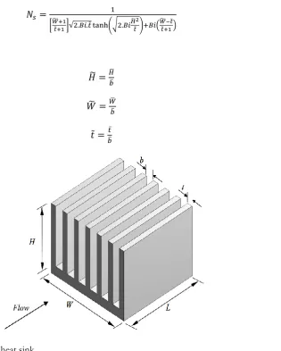
A typical plate fin heat sink is shown in Fig. 1. According to this figure, the fin thickness is t, fin spacing is b and the base of the heat sink is W x L. The heat sink base thickness is tb which is not shown in this figure.

For the shown heat sink under free convection or when the pressure drop is not a matter of

importance, the rate of entropy generation may be expressed as [21]:

𝑆̇_𝑔𝑒𝑛 =𝑄𝜃𝑏

𝑇∞2 (1)

where θb = Tb− T∞, is the difference between heat sink base temperature and ambient temperature.

Knowing Q = θb/Rsink

𝑆̇_𝑔𝑒𝑛 =𝑄2𝑅𝑠𝑖𝑛𝑘

𝑇∞2 ( 2)

𝑅_{𝑠𝑖𝑛𝑘} = 𝑁 1 𝑅𝑓𝑖𝑛+ℎ(𝑁−1)𝑏𝐿

+ 𝑡𝑏

𝑘𝐿𝑊 (3)

in which the second term is heat sink base thermal resistance. It is clear that this resistance is importance when the area of the heating source and heat sink are not the same and no minimum value can be found for this resistance. So, during the optimization procedure, it can be omitted without loss of generality. R_fin is fin thermal resistance and defined as [22]:

𝑅_𝑓𝑖𝑛 = 1

√ℎƤ𝑘𝐴𝑐tanh⁡(𝑚𝐻) (4)

𝑚 = √2ℎ_𝑘𝑡 (5)

where⁡Ƥ and A_c⁡are perimeter and cross section area of fin:

Ƥ = 2(𝐿 + 𝑡) ≈ 2L (6)

𝐴_𝑐 = 𝐿. 𝑡 (7)

So, the dimensionless form of Eq. (4) may be proposed as:

𝑅𝑓𝑖𝑛 = 1

𝑘𝐿√2.𝐵𝑖_𝑏𝑡̅_̅tanh(√2.𝐵𝑖𝐻̅ 2_𝑡̅𝑏̅)

(8)

in which over bar means dimensionless form of parameter i.e. t̅ = ⁡t

L or b̅ = ⁡ b L.

𝐵𝑖 =𝑁𝑢𝑘𝑓

𝑘 = ℎ𝑏

𝑘 (9)

and finally:

𝑅_{𝑠𝑖𝑛𝑘}= 1

𝑘𝐿[𝑁√2.𝐵𝑖𝑡̅_𝑏̅tanh⁡(√2.𝐵𝑖𝐻̅ 2_𝑡̅𝑏̅)+𝐵𝑖(𝑁−1)] (10)

and the rate of entropy generation may be redefined as:

𝑆̇𝑔𝑒𝑛 = 𝑄

2

𝑇_∞2_𝑘𝐿

1

[𝑁√2.𝐵𝑖_𝑏̅𝑡̅tanh⁡(√2.𝐵𝑖𝐻̅ 2_𝑡̅𝑏̅)+𝐵𝑖(𝑁−1)]

(11)

In this regard, the number of entropy generation can be proposed as:

𝑁_𝑠= 𝑆̇𝑔𝑒𝑛 𝑄 𝑇∞𝑘𝐿.

𝑄 𝑇∞

= 1

𝑁√2.𝐵𝑖_𝑏̅𝑡̅𝑡𝑎𝑛ℎ⁡(√2.𝐵𝑖𝐻̅ 2_𝑡̅𝑏̅)+𝐵𝑖(𝑁−1)

(12)

Based on heat sink geometry, one can present:

𝑁. 𝑡 + (𝑁 − 1). 𝑏 = 𝑊 (13)

or in the dimensionless form:

𝑁 =𝑊̅ +𝑏̅

𝑡̅+𝑏̅ (15)

𝑁 − 1 =𝑊_{𝑡̅+𝑏̅}̅ −𝑡̅ (16)

By replacing Eq. (15) and Eq. (16) in Eq. (12), the final form of the number of entropy generation will be:

𝑁𝑠 = 1

[𝑊̅̅̅+𝑏̅_{𝑡̅+𝑏̅}]√2.𝐵𝑖_𝑏𝑡̅_̅tanh⁡(√2.𝐵𝑖𝐻̅ 2_𝑡̅𝑏̅)+𝐵𝑖(𝑊̅̅̅−𝑡̅_{𝑡̅+𝑏̅})

(17)

To optimize the heat sink, it is just enough to minimize the number of entropy generation, Eq. (17). The effective variables in Eq. (17) are Bi, H̅, W̅, t̅ and b̅. However, considering the arrangement of variables in Eq. (17), it is clear that the number of variables can be reduced more by dividing geometrical parameters by b̅. In this way, Eq. (17) may be summarized as follows:

𝑁𝑠 = 1

[𝑊̃+1_𝑡̃+1]√2.𝐵𝑖.𝑡̃ tanh(√2.𝐵𝑖𝐻̃ 2_𝑡̃)+𝐵𝑖(𝑊̃−𝑡̃_𝑡̃+1)

(18)

where:

𝐻̃ =𝐻_𝑏̅̅ (19)

𝑊̃ =𝑊̅

𝑏̅ (20)

𝑡̃ =_𝑏̅𝑡̅ (21)

Fig. 1. A typical plate fin heat sink.

3.

Parametric Study

3.1. Effect of 𝐇̃ on Number of Entropy Generation

Figure 2 shows variation of number of entropy generation with H̃. By increasing Bi, N_s approaches to an asymptotic value. By increasing H̃, fin surface temperature approaches to ambient temperature. So, depending on Bi, no considerable heat transfer occurs from a longer fins and therefore, increasing the fin length does not affect number of entropy generation.

Fig. 2. Variation of number of entropy generation with 𝐻̃.

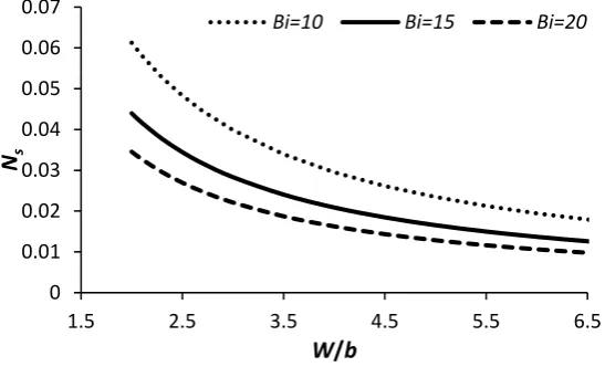
3.2. Effect of 𝐖̃ on Number of Entropy Generation

Figure 3 shows variation of number of entropy generation with W̃ . Increasing W̃ results in decreasing number of entropy generation, monotonically. Since by increasing the base heat sink dimension, W̃, the fin temperature decreases and therefore number of entropy generation decrease as a result.

Fig. 3. Variation of number of entropy generation with 𝑊̃.

3.3. Effect of 𝐁𝐢 on Number of Entropy Generation

The effect of Bi on number of entropy generation is shown in Fig. 4. By increasing Bi the number of entropy generation decreases monotonically. Since in higher Bi, heat transfer occurs at lower temperatures. It is important to note that by increasing Bi, its effect on the number of entropy generation decreases. It is because of this fact that at higher Bi, the conductive resistance of fins gets critical. Moreover, this figure shows that W̃ does not affect Ns significantly and for W̃ > 2, its effect cam be neglected.

0.6 0.7 0.8 0.9 1 1.1 1.2 1.3 1.4

0 0.5 1 1.5 2 2.5 3

Ns

H/b

Bi=0.05 Bi=0.07 Bi=0.1

0 0.01 0.02 0.03 0.04 0.05 0.06 0.07

1.5 2.5 3.5 4.5 5.5 6.5

Ns

W/b

Fig. 4. Variation of number of entropy generation with 𝐵𝑖.

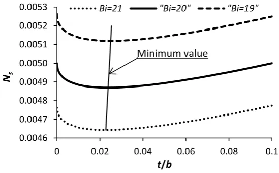
3.4. Effect of 𝐭̃ on Number of Entropy Generation

Figure 5 shows variation of number of entropy generation with t̃ for W̃ = 10 and H̃ = 2 . Based on this figure, by increasing t̃, Ns decreases rapidly to a minimum value and then increases slowly. So, if for any

reason, the optimum fin thickness is not accessible, it is just enough to be ensured that the thickness is more that the optimum value. Curves are plotted for three different Bi’s and the minimum values are connected to each others. In this regard, the optimum value of t̃ depends on⁡Bi also. The other point is that in higher values, the sensitivity of N_s to t̃ is lower. This, may be interpreted in this way that by increasing the fin thickness, the thermal conductive resistance decreases but on the other hand, increasing the fin thickness in the heat sink with constant width decreases the possible number of fins as well as total heat transfer area. Therefore, for a specified heat generation rate, higher temperature difference is required which means higher entropy generation rate. It is clear that in lower Bi, the role of convective heat transfer is weak, therefore the decrease of fin conductive thermal resistance in higher fin thickness is less effective.

Fig. 5. Variation of number of entropy generation with 𝑡̃.

4.

Geometry Optimization

Based on the performed parametric study, increasing all the variables with the exception of t̃, results in decreasing N_s. So, actually no optimum value may be found. But for the variable t̃, there is an optimum value. To find the optimum value of t̃, the denominator of Eq. (18) must be maximized or:

0 0.2 0.4 0.6 0.8 1 1.2 1.4

0 2 4 6 8

Ns

Bi

W/b=1 W/b=2 W/b=3

0.0046 0.0047 0.0048 0.0049 0.0050 0.0051 0.0052 0.0053

0 0.02 0.04 0.06 0.08 0.1

Ns

t/b

Bi=21 "Bi=20" "Bi=19"

𝑑 𝑑𝑡̃{[

𝑊̃ +1

𝑡̃+1] √2. 𝐵𝑖. 𝑡̃ tanh (√2. 𝐵𝑖 𝐻̃2

𝑡̃ ) + 𝐵𝑖 ( 𝑊̃ −𝑡̃

𝑡̃+1)} = 0 (22)

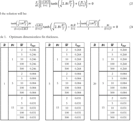
However, as it was shown, the value of W̃ on optimum value of t̃ is actually effectless. Eq. (22) was solved numerically by iterative method [23] for a large variety of H̃ ،Bi and W̃. Some results are presented in Table 1. As it can be observed, changing the value of W̃ from 2 to 500 does not affect the optimum dimensionless fin thickness. Owing to this fact, Eq. (22) may be approximate as:

𝑑 𝑑𝑡̃{[

√2.𝐵𝑖.𝑡̃

𝑡̃+1 ] tanh (√2. 𝐵𝑖 𝐻̃2

𝑡̃ ) + ( 𝐵𝑖

𝑡̃+1)} = 0 (23)

and the solution will be:

tanh(√2.𝐵𝑖𝐻̃ 2_𝑡̃).𝐵𝑖 (𝑡̃+1)√2.𝐵𝑖.𝑡̃ −

√2.𝐵𝑖.𝑡̃

(𝑡̃+1)2tanh (√2. 𝐵𝑖

𝐻̃2

𝑡̃) − 𝐵𝑖.𝐻̃

𝑡̃+1⁡

1−[tanh(√2.𝐵𝑖𝐻̃ 2_𝑡̃)]

2

𝑡̃ − 𝐵𝑖

(𝑡̃+1)2= 0 (24) Table 1. Optimum dimensionless fin thickness.

𝑯̃ 𝑩𝒊 𝑾̃ 𝒕̃𝑶𝒑𝒕 𝑯̃ 𝑩𝒊 𝑾̃ 𝒕̃𝑶𝒑𝒕 𝑯̃ 𝑩𝒊 𝑾̃ 𝒕̃𝑶𝒑𝒕

1 1

2 0.246

5 1

2 0.268

20 1

2 0.268

5 0.246 5 0.268 5 0.268

10 0.246 10 0.268 10 0.268

100 0.246 100 0.268 100 0.268

500 0.246 500 0.268 500 0.268

5

2 0.084

5

2 0.084

5

2 0.084

5 0.084 5 0.084 5 0.084

10 0.084 10 0.084 10 0.084

100 0.084 100 0.084 100 0.084

500 0.084 500 0.084 500 0.084

15

2 0.031

15

2 0.031

15

2 0.031

5 0.031 5 0.031 5 0.031

10 0.031 10 0.031 10 0.031

100 0.031 100 0.031 100 0.031

500 0.031 500 0.031 500 0.031

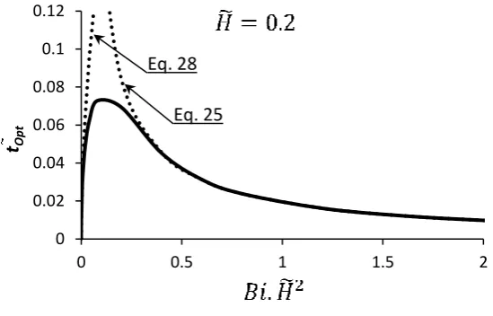
Unfortunately, no explicit results may be found for Eq. (24). Figure 6 and Figure 7 show the variation of t̃_opt as a function of dimensionless group, Bi⁡H̃2 _{for H̃ = 0.2 and H̃ = 1.0. As it can be observe, for the}

Fig. 6. Variation of 𝑡̃𝑜𝑝𝑡 with 𝐵𝑖⁡𝐻̃2 for 𝐻̃ = 0.2.

Fig. 7. Variation of 𝑡̃𝑜𝑝𝑡 with 𝐵𝑖⁡𝐻̃2 for 𝐻̃ = 1.0.

So, in the following, the optimum values of t̃opt for the limiting values of Bi⁡H̃2 are studied.

4.1. Limiting Case in which 𝐁𝐢. 𝐇̃𝟐_{→ ∞}

For this case:

lim⁡ 𝐵𝑖.𝐻̃2_→∞

⁡

tanh (√2. 𝐵𝑖𝐻̃_𝑡̃2) = 1 (25)

and the result of Eq. (24) is:

𝑡̃_∞= (1 + 𝐵𝑖) − √𝐵𝑖2_{+ 2𝐵𝑖 (26)}

4.2. Limiting Case in which 𝐁𝐢. 𝐇̃𝟐_{→ 𝟎}

For this case tanh (√2. BiH̃_t̃2) may be approximated by its Taylor series: 0

0.02 0.04 0.06 0.08 0.1 0.12

0 0.5 1 1.5 2

tOp

t Eq. 25

Eq. 28

0 0.05 0.1 0.15 0.2 0.25 0.3

0 2 4 6 8

tOp

t

Eq. 25

tanh (√2. 𝐵𝑖𝐻̃_𝑡̃2) ≈ √2. 𝐵𝑖𝐻̃_𝑡̃2−√2.𝐵𝑖 𝐻̃ 2

𝑡̃ 3

3 + O ([2. 𝐵𝑖 𝐻̃2

𝑡̃ ] 2

) (27)

[tanh (√2. 𝐵𝑖𝐻̃_𝑡̃2)]

2

≈ 2. 𝐵𝑖𝐻̃2

𝑡̃ (28)

By this approximation, the result of Eq. (24) is:

𝑡̃∞=2₃

𝐻̃(2.𝐵𝑖.𝐻̃2_{+√𝐵𝑖.𝐻̃}2_{(6+4.𝐵𝑖.𝐻̃}2_{)+3𝐵𝑖.𝐻̃)}

2𝐻̃+1 (29)

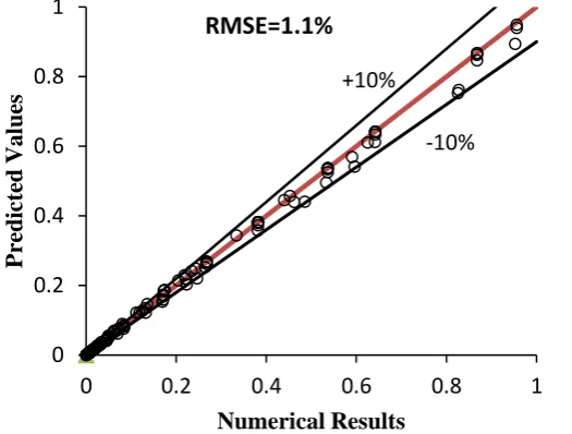
Eq. (22) was solved numerically for 220 different cases by means of Newton–Raphson method [23] and by using blending technique [24], the following equation was derived:

𝑡̃𝑂𝑝𝑡 = (𝑡̃∞−1+ 𝑡̃0−1)−1 (29)

The comparison of Eq. (30) against numerical results is shown in Fig. 8 which shows a good agreement.

Fig. 8. Comparison of predicted values against numerical results.

So, an explicit expression is proposed for optimum dimensionless thickness as a function of H̃ and⁡Bi. In the following the way of using Eq. (30) will be illustrated by means of several examples.

5.

Heat Sink Optimization under Natural Convection

The Nu for a plate fin heat sink in natural convection may be presented as follows [25]:

𝑁𝑢 =ℎ𝑏

𝑘𝑓 = (

576 (𝜂𝑓𝑖𝑛𝐸𝑙)2

+⁡ 2.873

(𝜂𝑓𝑖𝑛𝐸𝑙)0.5)

−1₂

(31)

in which

𝐸𝑙 = 𝑅𝑎. 𝑏4_⁄𝐿4 ₌𝑔𝛽𝜃𝑏𝑃𝑟𝑏4

𝐿𝜈2 = ⁡

𝑔𝛽𝜃𝑏𝑏4

𝐿𝜈𝛼 (32)

0 0.2 0.4 0.6 0.8 1

0 0.2 0.4 0.6 0.8 1

P

re

dic

ted

V

al

ues

Numerical Results

RMSE=1.1%

+10%

𝜂_𝑓𝑖𝑛 = tanh⁡(𝑚𝐻) 𝑚𝐻⁄ (33) and m can be calculated using Eq. (5).

 Example I: Optimizing fin thickness (1 geometrical parameter)

As a 1st example, consider a typical plate fin heat sink. Its geometrical parameters are specified in Table 2.

Table 2. Parameters of a plate fin heat sink n thickness.

W

(m) (m) H (m) L (m) tb (W/mK) k (K) θb T(K) amb (1/K)b (mn 2_/s) Pr Ra _(W/mK) kair

0.1 0.05 0.1 0.0015 200 55 300 0.0033 1.59E-05 0.707 5.03E+06 2.63E-02 Equationbs (30), (31) and (3) can be used to find the optimum thickness. The aforementioned equations are rearranged in the following:

𝑏 𝑡 =

3 2

2𝐻_𝑏+1

(𝐻_𝑏)(2.𝐵𝑖.(𝐻_𝑏)2+√𝐵𝑖.(𝐻_𝑏)2(6+4.𝐵𝑖.(𝐻_𝑏)2)+3𝐵𝑖.𝐻_𝑏)

+ 1

(1+𝐵𝑖)−√𝐵𝑖2_+2𝐵𝑖 (34)

𝐵𝑖 𝑘

𝑘𝑓= [

576

(𝑔.𝛽.𝑃𝑟.𝑏4_𝜐2.𝐿 𝜃𝑏

tanh(√2.𝐵𝑖𝐻2_𝑏.𝑡)

√2.𝐵𝑖𝐻_𝑏.𝑡2

⁡)

2+⁡ 2.873

(𝑔.𝛽.𝑃𝑟.𝑏4_𝜐2.𝐿 𝜃𝑏

tanh(√2.𝐵𝑖𝐻2_𝑏.𝑡)

√2.𝐵𝑖𝐻_𝑏.𝑡2 ) 0.5

]

−1₂

(35)

𝜃𝑏

𝑄 =

1

𝑘.𝐿[𝑊+𝑏_𝑡+𝑏]√2.𝐵𝑖_𝑏𝑡tanh⁡(√2.𝐵𝑖𝐻2_𝑏.𝑡)+𝐵𝑖(𝑊−𝑡_𝑡+𝑏)

+ 𝑡𝑏

𝑘.𝐿.𝑊 (36)

This system of equations involves three unknown variables i.e. t, b and Bi. The optimum thickness is found to be t_opt= 0.0005⁡m and the number of fins may be found according to Eq. (15).

𝑁 =𝑊+𝑏_𝑡+𝑏 =_0.0005+0.0060.1+0.006 = 16.31 ≈ 16 (37) The variation of heat transfer rate with number of fins are illustrated in Fig. 9 which shows good agreement with the found solution, N = 16.

44.0 46.0 48.0 50.0 52.0 54.0

12 14 16 18

Q

(W)

Fig. 9. Variation of heat transfer rate with number of fins.

 Example II: Optimizing fin height and spacing (2 geometrical parameters)

For the previous heat sink, it is now assumed that required heat generation rate and fin thickness are specified i.e. Q = 40⁡W and t = 3⁡mm. So, the optimum values are:

𝐵𝑖 = 0.00098 𝑏_𝑜𝑝𝑡= 0.028⁡𝑚

𝐻_𝑜𝑝𝑡= 0.125⁡𝑚

 Example III: Optimizing fin thickness and spacing (2 geometrical parameters)

This time, it is assumed that for the aforementioned heat sink, for the specified heat generation rate, the maximum working temperature is limited to 55 K. The optimum values are:

𝐵𝑖 = 0.00037 𝑏𝑜𝑝𝑡= 0.01⁡m

𝑡𝑜𝑝𝑡= 0.0018⁡m

6.

Heat Sink Optimization under Forced Convection

Because no specific assumption is made for Nu, Eq. (30) is still applicable for forced convection whenever the pressure drop is not a matter of importance (heat sinks of all small electronic devices such as CPU, may be included in this category). The Nu for a plate fin heat sink in forced convection may be presented as follows [26]:

𝑁𝑢 =ℎ𝑏_𝑘 𝑓 =

[ (𝑅𝑒𝑏∗𝑃𝑟

2 ) −3

+ (0.664√𝑅𝑒𝑏∗𝑃𝑟

1

3⁡⁡√1 + 3.65

√𝑅𝑒_𝑏∗) −3

]

−1₃

(38)

𝑅𝑒_𝑏∗_{= 𝑅𝑒}

𝑏(𝑏_𝐿) =𝑏.𝑉_𝜈𝑐ℎ(𝑏_𝐿) (39)

The total pressure drop of fluid flowing through a plate fin heat sink is [27]:

∆𝑃 = (𝐾_𝑐+ 𝐾_𝑒+𝑓𝑎𝑝𝑝𝐿(2𝐻+𝑏)

𝑏𝐻 ) 1 2𝜌𝑉𝑐ℎ

2 ₍₄₀₎

Chanel velocity is related to free stream velocity by:

𝑉_𝑐ℎ= 𝑉_𝑓(1 +𝑡

𝑏) (41)

Kc and Ke are sudden contraction and expansion pressure drop coefficient as defined as [28]:

𝐾𝑐 = 0.42(1 + 𝜎2) (42)

𝐾𝑒= (1 − 𝜎2)2 (43)

and σ is the plate fin heat sink porosity,

𝜎 = 1

(1+_𝑏𝑡) (44)

𝑓_𝑎𝑝𝑝𝑅𝑒_𝑐ℎ= [(3.44

√𝐿_𝑐ℎ∗ ) 2

+ (𝑓𝑅𝑒_𝑐ℎ)2_]

1 2

(45)

𝐿∗_𝑐ℎ=_𝐷 𝐿

𝑐ℎ𝑅𝑒𝑐ℎ (46)

𝑅𝑒𝑐ℎ=𝜌𝑉𝑐ℎ_𝜇𝐷𝑐ℎ (47)

𝐷𝑐ℎ≈ 2𝑏 (48)

𝑓𝑅𝑒_𝑐ℎ= 24 − 32.527 (𝑏

𝐻) + 46.721 ( 𝑏 𝐻)

2

− 40.829 (𝑏

𝐻) 3

+ 22.954 (𝑏

𝐻) 4

− 6.089 (𝑏

𝐻) 5

(49)

 Example IV: Optimizing fin thickness (1 geometrical parameter)

As an example, consider again the plate fin heat sink specified in Example I and Table 2 but under forced convection. The air velocity exiting the fan is assumed 2 m/s. Accordingly, the optimum thickness is topt=

0.001⁡m and the number of fins is: 𝑁 =𝑊+𝑏

𝑡+𝑏 =

0.1+0.006

0.001+0.006= 15.1 ≈ 15 (50)

The variation of heat transfer rate with number of fins is illustrated in Fig. 10 and shows good agreement with the found solution, N = 15.

Fig. 10. Variation of heat transfer rate with number of fins.

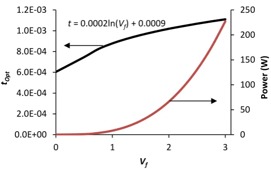
This problem is repeated for other velocities and results are illustrated in Fig. 11. 100

110 120 130 140 150 160 170 180

8 10 12 14 16 18

Q

(W

)

Fig. 11. Variation of 𝑡𝑜𝑝𝑡 and power consumption with 𝑉𝑓.

 Example V: Optimizing fin height and spacing (2 geometrical parameters)

It is now assumed that required heat generation rate and fin thickness are specified and i.e. Q = 40⁡W and t = 3⁡mm. So, the optimum values are:

𝐵𝑖 = 0.0015 𝑏_𝑜𝑝𝑡= 0.015⁡𝑚

𝐻_𝑜𝑝𝑡= 0.035⁡𝑚

which shows that shorter fin with larger fin spacing is required in comparison with natural convection.

 Example VI: Optimizing fin number using fan curve

In Example IV, air approach velocity was specified at first. However, it is clear that this velocity depends on the type of fan as well as pressure drop. So, it is more realistic to specify fan curve, instead. Fig. 12 shows the inverse relation between pressure drop and approach velocity for ETRI-DC-373DH fan. The pressure drop for various numbers of fins is also shown in this figure. The intersections between these curves show the system operating points.

Fig. 12. Operating points for various fin thickness.

The following simple curve can be fitted to the locus of operating points:

𝑉_𝑓 =_{0.9515+121.31𝑡}1 (51)

t = 0.0002ln(Vf) + 0.0009

0 50 100 150 200 250

0.0E+00 2.0E-04 4.0E-04 6.0E-04 8.0E-04 1.0E-03 1.2E-03

0 1 2 3

Pow

e

r (

W)

tOp

t

Vf

0 10 20 30 40 50

0.2 0.4 0.6 0.8 1 1.2

Δ

P (Pa)

Vf (m/s)

Knowing the approach velocity as a function of fin thickness, the following optimized results are obtained:

𝑄 = 252.7⁡𝑊 𝑡_𝑜𝑝𝑡= 0.00045⁡𝑚

∆𝑃 = 5.3⁡𝑃𝑎 𝑉_𝑓 = 0.994⁡𝑚/𝑠

7.

Conclusions

In the present study, by using the entropy generation minimization method, a general equation was proposed to relate the dimensionless parameters of the plate fin heat sink in optimum working condition. The importance of this work is that it has been based on dimensionless parameters. So the results are not limited to a specific geometry or some special examples. Moreover, since no restricting assumption was made, this equation can be used for both natural and forced convection. Six examples were employed to clear the method of using the proposed equation. Although the manufacturing process of a heat sink is always accompanied with many different restrictions such as machining tools, those examples showed that this method had enough flexibility to consider all these restrictions. It was shown also that how to use a fan curve instead of approach velocity in optimizing heat sink. Although considering fan curve is a little more difficult in comparison, it must be kept in mind that it is more realistic. Because the volumetric flow rate as well as approach velocity in a fan are also, functions of pressure drop and it is only a simplification to evaluate the flow rate independence of pressure drop.

Acknowledgments

The author would like to thank Islamic Azad University, Marvdasht branch for supporting this research project.

Nomenclature

𝐴𝑐= 𝐿. 𝑡 (m2) Cross section area of fin

𝑏 (m) Fin spacing

𝑏̅ = ⁡𝑏

𝐿 --- Dimensionless Fin spacing

𝐵𝑖 =𝑁𝑢𝑘𝑓

𝑘 =

ℎ𝑏

𝑘 --- Biot Number

El --- Elenbass Number

𝑓_𝑎𝑝𝑝 --- Apparent friction factor

H (m) Fin height

𝐻̅ = ⁡𝐻

𝐿 --- Dimensionless fin height

H (W/m2K) Convection heat transfer coefficient 𝐾𝑐 --- Sudden contraction pressure drop _coefficient

𝐾_𝑒 --- Sudden expansion pressure drop coefficient

𝑘 (W/mK) Heat sink thermal conductivity

𝑘𝑓 (W/mK) Fluid thermal conductivity

L (m) Heat sink Length

N --- Fin Number

𝑁𝑢 =ℎ𝑏

𝑘_𝑓 --- Nusselt Number

Ƥ = 2(𝐿 + 𝑡) ≈ 2L (m2_{) Perimeter of fin}

Q (W) Heat transfer rate

Rfin (K/W) Fin thermal resistance

𝑅𝑠𝑖𝑛𝑘 (K/W) Heat sink thermal resistance

𝑆̇_𝑔𝑒𝑛 (W/K) Rate of entropy generation

𝑇_∞ (K) Ambient temperature

𝑡 (m) Fin thickness

𝑡_𝑏 (m) Heat sink base thickness

𝑡𝑜𝑝𝑡 (m) Optimum fin thickness

𝑡̅ = ⁡𝑡

𝐿 --- Dimensionless thickness

𝑉_𝑐ℎ (m/s) Channel velocity

𝑉_𝑓 (m/s) Free stream velocity

W (m) Heat sink width

𝑊̅ =⁡𝑊

𝐿 --- Dimensionless heat sink width

𝜂_𝑓𝑖𝑛 --- Fin efficiency

𝜃_𝑏 = 𝑇_𝑏− 𝑇_∞ (K) Temperature difference

𝜎 --- Heat sink porosity

References

[1] P. Teertstra, M. M. Yovanovich, and J. R. Culham, “Analytical forced convection modeling of plate fin heat sinks,” in Semiconductor Thermal Measurement and Management Symposium, Fifteenth Annual IEEE, 1999, pp. 34–41.

[2] S. Y. Kim and R. L. Webb, “Analysis of convective thermal resistance in ducted fan heat sinks,” IEEE Transactions on Components and Packaging Technologies, vol. 29, pp. 439–448, 2006.

[3] C. J. Kobus and T. Oshio, “Development of a theoretical model for predicting the thermal performance characteristics of a vertical pin-fin array heat sink under combined forced and natural convection with impinging flow,” Int. J. Heat Mass Transfer, vol. 48, pp. 1053–1063, 2005.

[4] S. Chingulpitak, N. Chimresa, K. Nilpueng, and S. Wongwises, “Experimental and numerical investigations of heat transfer and flow characteristics of cross-cut heat sinks,” Int. J. Heat Mass Transfer, vol. 102, pp. 145–153, 2016.

[5] J. Hoa, K. Wonga, K. Leonga, and T. Wong, “Convective heat transfer performance of airfoil heat sinks fabricated by selective laser melting,” Int. J. Therm. Sci., vol. 114, pp. 213–228, 2017.

[6] S. Huanga, J. Zhaob, L. Gong, and X. Duana, “Thermal performance and structure optimization for slotted microchannel heat sink,” Appl. Therm. Eng., vol. 115, pp. 1266–1276, 2017.

[7] S. B. Sathe, “An analytical study of the optimized performance of an impingement heat sink,” J. Electron. Packaging, vol. 126, pp. 528–534, 2004.

[8] O. Leon, “Comparison between the standard and staggered layout for cooling fins in forced convection cooling,” J. Electron. Packaging, vol. 125, pp. 442–446, 2003.

[9] P. H. Oosthuizen, “A numerical study of mixed convective heat transfer from a parallel fin heat sink,” in 38th _{AIAA Thermophysics Conference, Toronto, Ontario Canada, AIAA, 2005, p. 4824.}

[10] A. Z. Sahin, “Second law analysis of laminar viscous flow through a duct subjected to constant wall temperature,” Int. J. Heat Mass Transfer, vol. 120, pp. 76–83, 1998.

[11] S. Mahmud and R. A. Fraser, “The second law analysis in fundamental convective heat transfer problems,” Int. J. Therm. Sci., vol. 42, pp. 177–186, 2003.

[12] S. Z. Shuja and B. S. Yilbas, “Flow through a protruding bluff body-heat and irreversibility analysis,” Exergy, vol. 1, pp. 209–215, 2001.

[13] A. C. Baytas, “Entropy generation for natural convection in an inclined porous cavity,” Int. J. Heat Mass Transfer, vol. 43, pp. 2089–2099, 2000.

[14] I. Dagtekin, H. F. Oztop, and A. Z. Sahin, “An analysis of entropy generation through a circular duct with different shaped longitudinal fins for laminar flow,” Int. J. Heat Mass Transfer, vol. 48, pp. 71–181, 2005.

[16] C. J. Shih and G. C. Liu, “Optimal design methodology of plate-fin heat sinks for electronic cooling using entropy generation strategy,” IEEE Trans. Compon. Packag. Technol., vol. 27, no. 3, pp. 551–559, 2004.

[17] J. Culham and Y. Muzychka, “Optimization of plate fin heat sinks using entropy generation minimization,” IEEE Trans. Compon. Packag. Technol., vol. 24, vol. 159–165, 2001. Available: http://dx.doi.org/10.1109/6144.926378

[18] W. Khan, J. Culham, and M. Yovanovich, “Optimization of pin-fin heat sinks using entropy generation minimization,” IEEE Trans. Compon. Packag. Technol., vo. 28, pp. 247–254, 2005.

[19] W. Khan and J. Culham, “The role of fin geometry in heat sink performance,” J. Electron. Packaging, vol. 128, pp. 324–330, 2006.

[20] M. Asadi and A. Shalchi-Tabrizi, “Introducing some correlations to calculate entropy generation in extended surfaces with uniform cross sectional area,” Phys. Sci. Int. J., vol. 4, no. 3, pp. 402–415, 2014. [21] A. Bejan and E. Sciubba, “The optimal spacing of parallel plates cooled by forced convection,” Int. J.

Heat Mass Transfer, vol. 35, pp. 3259–3264, 1992.

[22] F. P. Incropera and D. P. Dewitt, Fundamentals of Heat and Mass Transfer. New York: Wiley, 1996. [23] W. F. Stoecker, Design of Thermal Systems. 3rd ed. McGraw Hill, 1989.

[24] S. W. Churchill and R. Usagi, “A general expression for the correlation of rates of transfer and other phenomena,” A.I.Ch.E. JI, vol. 18, pp. 1121–1128, 1972.

[25] S. Barcohen and W. Rohsenow, “Thermal optimum spacing of vertical natural convection cooled parallel plates,” J. Heat Treansf, vol. 106, pp. 116–123, 1984.

[26] P. M. Teertstra, M. M. Yovanovich, J. R. Culham, and T. F. Lemczyk, “Analytical forced convection modeling of plate fin heat sinks,” in Proc. 15th _{Annu. IEEE Semicon. Thermal Meas. Manag. Symp., San}

Diego, CA, March 9–11, 1999, pp. 34–41.

[27] W. M. Kays, and A. L. London, Compact Heat Exchangers. New York: McGraw-Hill, 1984. [28] F. M. White, Fluid Mechanics. New York: McGraw-Hill, 1987.