Model Selection with Application to Gamma Process and Inverse
Gaussian Process
M. Zhang & M. Revie
Department of Management Science University of Strathclyde, Glasgow, UK
ABSTRACT: The gamma process and the inverse Gaussian process are widely used in condition-based main-tenance. Both are suitable for modelling monotonically increasing degradation processes. One challenge for practitioners is determining which of the two processes is most appropriate in light of a real data set. A common practice is to select the one with a larger maximized likelihood. However, due to variations in the data, the max-imized likelihood of the “wrong” model could be larger than that of the “right” model. This paper proposes an efficient and broadly applicable test statistic for model selection. The construction of the test statistic is based on the Fisher information. Extensive numerical study is conducted to indicate the conditions under which the gamma process can be well approximated by the inverse Gaussian process, or the other way around.
1 INTRODUCTION
The gamma process and the inverse Gaussian process were proposed by Dufresne et al. (1991) and Wasan (1968), respectively. Dufresne et al. (1991) proved that a gamma process is a limit of compound Pois-son processes. They also constructed an inverse Gaus-sian process from compound Poisson processes. The gamma and inverse Gaussian processes are widely used for modeling degradation data. Various main-tenance strategies developed in the literature when degradation data are modelled by the gamma process can be found in Zhang and Zhou (2014), Zhang et al. (2014) and Zhu et al. (2015). van Noortwijk (2009) provided an excellent review on the gamma process. Applications and generalizations of the inverse Gaus-sian process can be found in Al Labadi and Zarepour (2013), Griffin et al. (2013) and Tang et al. (2009).
Mathematically, the gamma distribution with shape parameterα (>0)and scale parameterβ (>0), de-noted byGa(α, β), has probability density function fGa(x; α, β) =
βα
Γ(α)x
α−1exp(−βx), x >0.
Here Γ(α) is the gamma function evaluated at α. The cumulative distribution function is the regular-ized gamma function:
FGa(x; α, β) =
Z x
0 βα
Γ(α)y
α−1
exp(−βy)dy
=γ(α, βx)/Γ(α), x >0.
Hereγ(α, βx)is the lower incomplete gamma func-tion. The mean and variance of the gamma distribu-tion are αβ−1 and αβ−2, respectively. A stochastic process{X(t), t≥0}is a gamma process if
• non-overlapping increments are independent;
• ∀t > s≥0, the random incrementX(t)−X(s)
has the gamma distributionGa(α(t−s), β). The marginal distribution of the gamma process
{X(t), t ≥ 0} at time t is the gamma distribution Ga(αt, β). {X(t), t ≥ 0} is a stationary process having mutually independent, stationary and non-negative increments.
The inverse Gaussian distribution with meanu(>
0)and shape parameterλ(>0), denoted byIG(u, λ), has probability density function
fIG(x; u, λ) =
s λ
2πx3exp −
λ(x−u)2
2u2x !
, x >0,
and cumulative distribution function FIG(x; u, λ) = exp(2λ/u)Φ
− s
λ x
x u+ 1
+Φ
s
λ x
x u−1
, x >0.
HereΦ(·)is the standard normal cumulative distribu-tion funcdistribu-tion. The variance of the inverse Gaussian distribution isu3/λ. A stochastic process{Y(t), t≥
• non-overlapping increments are independent;
• ∀t > s≥0, the random incrementY(t)−Y(s)
has the inverse Gaussian distribution IG(u(t−
s), λ(t−s)2).
Therefore, the marginal distribution of the inverse Gaussian process{Y(t), t≥0}at timetis the inverse Gaussian distributionIG(ut, λt2). {Y(t), t ≥0}is a stationary process of which the increments are mu-tually independent, stationary and non-negative.
Both the gamma process and the inverse Gaussian process are suitable for modeling gradual damage in-troduced by continuous use. Therefore, given degra-dation data, the uppermost problem is selecting be-tween the two processes the “right” model. A com-mon practice is to select the one with a larger maxi-mized likelihood. However, due to the variation in the data, the maximized likelihood of the “wrong” model is probably larger than that of the “right” model. In order to reduce the probability of selecting a wrong model, the data size should be sufficiently large. This paper proposes an efficient and broadly applicable test statistic for model selection by quoting the the-orems in White (1982). The problem of model selec-tion or model-misspecificaselec-tion detecselec-tion has received much attention. A representative sample of works on model selection or model-misspecification detection includes Hyodo et al. (2012), Tsai et al. (2011) and Zhou et al. (2012). Note that, to select a model for the underlying degradation process is essentially to select a distribution for the degradation increments. There-fore, in what follows we focus on selecting between the gamma distribution and the inverse Gaussian dis-tribution the right one for collected degradation data.
The remainder of the paper is organised as fol-lows. Section 2 derives a general expression of the test statistic when the underlying stochastic law is unspec-ified. Section 3 conducts extensive numerical study to demonstrate the efficiency of the test statistic. Con-clusions are outlined in Section 4.
2 A GENERAL FRAMEWORK
Due to the lack of space, we explain our idea by tak-ing the gamma process as an example. For the inverse Gaussian process, the appropriate translations are ob-vious.
We might assume that the underlying degradation process is stationary. Hence both the inverse Gaus-sian process and the gamma process are suitable for fitting the degradation measurements. The following data-collecting scheme will be adopted. LetX(t) de-note the degradation of a target device measured at time t, with X(0) = 0. The degradation of the de-vice is measured every ∆(> 0) units of time. The data-collecting scheme is terminated at time n∆, n = 1,2, .... Denote the collected degradation data by Xn = {x1, x2, ..., xn} in which xi = X(i∆)−
X((i−1)∆), i = 1,2, ..., n. The independent ran-dom increments {x1, x2, ..., xn} have the same
dis-tribution function, denoted by G(x), x > 0. G(x) is the unknown underlying stochastic law. Let g(x) de-note the corresponding probability density function. We below approximateG(x)by the gamma distribu-tion,Ga(α∆, β). To simplify the notation which fol-lows, define two vectors of parameters:θ= (θ1, θ2) =
(α∆, β)andϑ= (ϑ1, ϑ2) = (u∆, λ∆2).
Given the degradation data Xn, consider a quasi
log-likelihood function ofθ:
`Ga(θ; Xn) =
1
n
n
X
k=1
log(fGa(xk; θ))
= n−1
n
X
k=1
[(θ1−1) log(xk)−θ2xk]
+θ1log(θ2)−log(Γ(θ1)).
Find a value of θ that maximizes `Ga(θ; Xn).
De-note the maximizer by θˆ= (ˆθ1, θˆ2). θˆ is termed as the quasi maximum-likelihood (QML) estimator for θ. Notably, given the data Xn, n`Ga(θ; Xn) =
n
P
k=1
log(fGa(xk; θ)) is the log-likelihood function
of θ. Hence, the QML estimator θˆ is indeed the maximum-likelihood estimator forθ. The maximized quasi log-likelihood`Ga( ˆθ; Xn)is exactly1/nof the
maximized log-likelihood. The QML estimator forθ2 has a closed form: θˆ2 =nθˆ1/
n
P
k=1
xk. The QML
esti-mator forθ1, i.e.θˆ1, is the solution of
log(θ1)−ψ(θ1) = log
1
n
n
X
k=1 xk
!
− 1
n
n
X
k=1
log(xk),
which can be solved numerically. Here, ψ(θ1) is the digamma function evaluated atθ1.
The Kullback-Leibler divergence (Kullback and Leibler 1951) is a non-symmetric measure of the dif-ference between two probability distributions. As-sume that G1 and G2 are two probability measures over a setS, andG1 is absolutely continuous with re-spect toG2. The measure is non-symmetric in that the Kullback-Leibler divergence of G1 from G2 is most often different from the Kullback-Leibler divergence of G2 from G1. The Kullback-Leibler divergence of G2fromG1is defined to be
I(G2, G1) = Z
S
log(dG1/dG2)dG1.
The Kullback-Leibler divergence of FGa(x; θ)
fromG(x)is
I(FGa, G) = E[log(g(x)/fGa(x; θ))]
= E[log(g(x))]−E[log(fGa(x; θ))].
Here, and in what follows, expectations are all taken with respect to the true stochastic lawg(x). The first term of the right-hand side, i.e. E[log(g(x))], is in-dependent of θ. The minimization of I(FGa, G) is
equivalent to the maximization ofE[log(fGa(x; θ))].
Notably, the quasi log-likelihood `Ga(θ; Xn) is a
(strongly) consistent estimator forE[log(fGa(x; θ))].
Letθ∗ denote the optimal parameter vector minimiz-ing the Kullback-Leibler divergence:
θ∗ = arg min
θ>0 I(FGa, G) = arg maxθ>0 E[log(fGa(x; θ))]. If the stochastic law lies within the family of gamma distributions (i.e.,g(x) =fGa(x; θ0)for some
θ0 > 0), then I(FGa, G) attains its unique
mini-mum at θ∗ = θ0. The value of θ∗
is inaccessible. Because `Ga(θ; Xn) is a consistent estimator for
E[log(fGa(x; θ))], one may conjecture that θˆ is a
consistent estimator forθ∗.
Define two2×2matricesAGa(θ)andBGa(θ):
[AGa(θ)]ij =E
"
∂2log(f
Ga(x; θ))
∂θi∂θj
# ,
and
[BGa(θ)]ij =E
"
∂log(fGa(x; θ))
∂θi
∂log(fGa(x; θ))
∂θj
# .
Here, we have utilized the fact that differentiation can be taken inside integral. AGa(θ) and BGa(θ)
can be respectively consistently estimated by matri-cesAn
Ga(θ)andBGan (θ):
[AnGa(θ)]ij =n−1 n
X
k=1
∂2log(fGa(xk; θ))
∂θi∂θj
,
and
[BGan (θ)]ij =
n−1
n
X
k=1
∂log(fGa(xk; θ))
∂θi
∂log(fGa(xk; θ))
∂θj
.
If the matrices AGa(θ) and AnGa(θ) are invertible,
which can always be guaranteed, define CGa(θ) =AGa(θ)−1BGa(θ)AGa(θ)−1,
and
CGan (θ) =AnGa(θ)−1BGan (θ)AnGa(θ)−1.
The superscript “-1” above a matrix denotes the in-verse operator. Cn
Ga(θ) is a consistent estimator for
CGa(θ).
Proposition 1 The distribution of √n( ˆθ −θ∗) is
asymptotically normal with mean zero and covari-ance matrix CGa(θ∗). The sequence CGan ( ˆθ)
con-verges almost surely towards CGa(θ∗): CGan ( ˆθ) a.s.
→
CGa(θ∗), element by element. Specifically, if g(x) =
fGa(x; θ0)for someθ0 >0, then
• θˆis a (strongly) consistent estimator forθ0;
• √n( ˆθ−θ0)is asymptotically normal with mean zero and covariance matrixCGa(θ0).
Proof. The assumptions A1-A6 in White (1982) all hold. The proposition follows from Theorem 3.2 of White (1982), and the proof is complete.
If the underlying stochastic law is correctly spec-ified and if differentiation can be taken inside inte-gral, the information matrix can be expressed in either the Hessian form, i.e.−AGa(θ0), or the outer product
form, i.e. BGa(θ0). The information-matrix
equiva-lence indicates that the sumAGa(θ0) +BGa(θ0)can
be used for detecting model misspecification. Specif-ically, the failure of the sum AGa(θ∗) +BGa(θ∗)
equalling zero states that the stochastic law is mis-specified. The values of the elements in AGa(θ∗) +
BGa(θ∗) are inaccessible. Yet, by Proposition 1,
AGa(θ∗) +BGa(θ∗)can be consistently estimated by
An
Ga( ˆθ) +BGan ( ˆθ). Hence, the remaining work is to
investigate the distributional property of the elements inAn
Ga( ˆθ) +BGan ( ˆθ).
Define a vector-valued function: δGa(x; θ) =
(δ1(x; θ), δ2(x; θ), δ3(x; θ))tin which δ1(x; θ) =
∂log(fGa(x; θ))
∂θ1
∂log(fGa(x; θ))
∂θ1
+∂
2log(f
Ga(x; θ))
∂θ1∂θ1 ,
δ2(x; θ) =
∂log(fGa(x; θ))
∂θ1
∂log(fGa(x; θ))
∂θ2
+∂
2log(f
Ga(x; θ))
∂θ1∂θ2 , and
δ3(x; θ) =
∂log(fGa(x; θ))
∂θ2
∂log(fGa(x; θ))
∂θ2
+∂
2log(f
Ga(x; θ))
∂θ2∂θ2 .
By the superscript “t”, we mean the transpose of a vector or a matrix. Define
¯
δGan (θ) =n−1
n
X
k=1
¯
δn
Ga( ˆθ) consists of all the distinct elements in
An
Ga( ˆθ) +BGan ( ˆθ). Hence, we below investigate the
asymptotic joint distribution of δ¯Gan ( ˆθ). Take expec-tation ofδGa(x; θ)with respect tog(x):
¯
δGa(θ) = E[δGa(x; θ)]
= (E[δ1(x; θ)], E[δ2(x; θ)], E[δ3(x; θ)])t.
The respective3×2Jacobian matrices of the vector-valued functionsδ¯n
Ga(θ)andδ¯Ga(θ)are
[JGan (θ)]ij =n−1 n
X
k=1
∂δi(xk; θ)
∂θj
,
and
[JGa(θ)]ij =
∂E[δi(x; θ)]
∂θj
=E "
∂δi(x; θ)
∂θj
# .
The partial derivative with respect to θ of the loga-rithm offGa(x; θ)is
∇log(fGa(x; θ))
= ∂log(fGa(x; θ))
∂θ1
, ∂log(fGa(x; θ)) ∂θ2
!t .
The nabla symbol “∇” denotes the vector differential operator. Define two3×3matrices
VGa(θ) =E[vGa(x; θ)vGa(x; θ)t],
and
VGan(θ) =n−1
n
X
k=1
¨
vGa(xk; θ) ¨vGa(xk; θ)t.
The column vectors vGa(x; θ) and v¨Ga(xk; θ) are
defined by
vGa(x; θ) =δGa(x; θ)
−JGa(θ)AGa(θ)−1∇log(fGa(x; θ)),
and
¨
vGa(xk; θ) =δGa(xk; θ)
−JGan (θ)AnGa(θ)−1∇log(fGa(xk; θ)).
Proposition 2 Ifg(x) =fGa(x; θ0)for someθ0>0,
then
• √nδ¯n
Ga( ˆθ) is asymptotically normally
dis-tributed with mean zero and covariance matrix VGa(θ0);
• the sequenceVn
Ga( ˆθ)converges almost surely to
VGa(θ0);
• Vn
Ga( ˆθ)is nonsingular almost surely for all
suffi-ciently largen;
• the asymptotic distribution of the test statistic ζn
Ga =nδ¯Gan ( ˆθ)tVGan ( ˆθ)
−1δ¯n
Ga( ˆθ) is chi-squared
distribution with three degrees of freedom. Proof. The assumptions A1-A10 in White (1982) all hold. The proposition follows from Theorem 4.1 of White (1982), and the proof is complete.
ζn
Ga serves as a test statistic in a hypothesis test. A
hypothesis test can be constructed with the null hy-pothesis given by
H0 : g(x) =fGa(x; θ), ∃θ>0
and the alternative hypothesis given by H1: g(x)6=fGa(x; θ), ∀θ>0.
If the null hypothesis is true, the test statistic ζGan is chi-squared distributed with three degrees of freedom. To carry out the test, one calculatesζGan and compares it to the critical value of theχ2
3distribution. IfζGan
ex-ceeds the critical value, one rejects the null hypothesis and concludes that the specified family of probability distributions is inappropriate. If the null hypothesis is accepted, one may have confidence that the estimators will be consistent for parameters of interest. Note that ζn
Gaalso measures how well the density functiong(x)
could be approximated by a gamma density function. Specifically, for a given sample sizen, the smaller the value ofζGan , the better the density functiong(x)could be approximated by a gamma density function. 3 NUMERICAL EXAMPLES
3.1 Fit Data by the Gamma Process
Assume that the underlying stochastic law is an in-verse Gaussian process. Randomly simulaten obser-vations, denoted by Xn, from the inverse Gaussian
distribution fIG(x; ϑ). Fit the gamma distribution
to the data Xn. Maximize the quasi log-likelihood
`Ga(θ; Xn) to obtain the QML estimate ofθ, i.e. θˆ.
The corresponding maximized quasi log-likelihood is denoted by `nθˆ. Given the data Xn and the QML
es-timate θˆ, calculate the value of the test statistic ζGan . For comparison, fit the inverse Gaussian distribution to the data Xn, maximize the quasi log-likelihood
`IG(ϑ; Xn), and denote the maximized quasi
log-likelihood by`nϑˆ. Define a statisticτn:
τn=P
`nθˆ> `nϑˆ=Pn`nθˆ> n`nϑˆ.
A common practice for model selection is comparing the maximized log-likelihoods: n`n
ˆ
θ andn` n
ˆ
ϑ. Hence,
for a given sample sizen, τn is the probability of
For illustrative purpose, we increase the shape pa-rameter ϑ2 from 0.2 to 6 with step size 0.2. Fix the meanϑ1 at 10. Gradually increase the sample size n from 10 to 100 with step size 5. For each combination ofϑ2 andn, we generate 1000 data sets. Calculate`nθˆ, `nϑˆ and ζGan for each data set. For the 1000 pairs of n
`n
ˆ
θ, ` n
ˆ
ϑ
o
, calculate the percentage of`n
ˆ
θ being larger
than`n
ˆ
ϑ. The percentage is an estimate ofτn. Take
av-erage of the 1000 values ofζn
Ga. The critical value of
the chi-square distribution with 3 degrees of freedom at significance level 0.05 is 7.815.
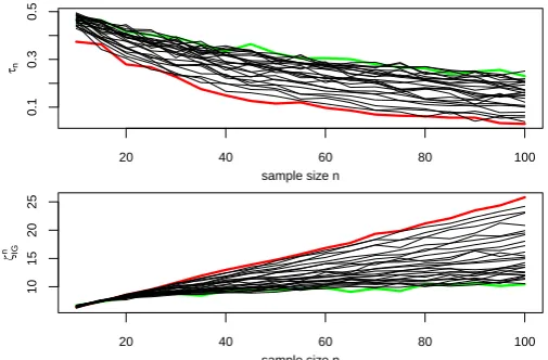
Plot the evolution of τn and the averaged value of
ζn
Ga in Figure 1. In Figure 1, the red curve
corre-20 40 60 80 100
0.00
0.10
0.20
sample size n
τn
20 40 60 80 100
10
20
30
40
sample size n
ζGa
[image:5.595.34.288.238.402.2]n
Figure 1: The evolution ofτn(above) and the averaged value of
ζn
Ga(blow).
sponds toϑ2 = 0.2, and the green curve corresponds toϑ2 = 6. Figure 1 shows that, if the shape parameter ϑ2is relatively large, the inverse Gaussian distribution can be closely approximated by a gamma distribution. To guarantee a 0.95 probability of selecting the right model,τnshould be smaller than 0.05. We let n1
de-note the sample size, beyond which the value ofτnis
smaller than 0.05; letn2 denote the sample size, be-yond which the averaged value of ζn
Ga is larger than
[image:5.595.309.562.508.674.2]7.815. The evolution of n1 and n2 along with ϑ2 is summarized in Table 1. Table 1 shows that selecting
Table 1: The required sample size for selecting the right model with probability 0.95.
ϑ2 n1(τn) n2(ζGan ) ϑ2 n1(τn) n2(ζGan )
0.2 20 20 3.4 30 35
0.6 20 20 3.8 35 35
1.0 20 25 4.2 35 40
1.4 25 25 4.6 40 40
1.8 25 30 5.0 45 45
2.2 30 30 5.4 45 45
2.6 35 35 5.8 45 45
3.0 30 35 6.0 45 45
model according to maximized log-likelihoods is as efficient as selecting model according to the proposed test statistic.
3.2 Fit Data by the inverse Gaussian Process Assume that the underlying stochastic law is a gamma process. Randomly simulate n observations from the gamma distribution fGa(x; θ). Fit the inverse
Gaussian distribution to the data Xn. Maximize the
quasi log-likelihood to obtain the QML estimate of
ϑ, i.e. ϑˆ. The corresponding maximized quasi log-likelihood is denoted by`n
ˆ
ϑ. Given the dataXnand the
QML estimateϑˆ, calculate the value of the test statis-ticζIGn . For comparison, fit the gamma distribution to the data Xn, maximize the quasi log-likelihood, and
denote the maximized quasi log-likelihood by`nθˆ. De-fine a statisticτn:
τn=P
`nϑˆ> `nθˆ
=Pn`nϑˆ > n`nθˆ
.
For a given sample sizen,τnis the probability of
se-lecting the wrong model, if we select by comparing maximized log-likelihoods.
For illustrative purpose, we increase the shape pa-rameter θ1 from 1.8 to 7 with step size 0.2. (Exper-iments showed that, when θ1 < 1.8 and n is small, the matrixVIGn( ˆϑ)is likely to be singular. Hence, we start from 1.8 instead of from 0.2.) Fix the scale pa-rameter θ2 at 1. Gradually increase the sample size nfrom 10 to 100 with step size 5. For each combina-tion ofθ1andn, we generate 1000 data sets. Calculate `n
ˆ
ϑ,` n
ˆ
θ andζ n
IG for each data set. For the 1000 pairs of
n `n
ˆ
ϑ, ` n
ˆ
θ
o
, calculate the percentage of`n
ˆ
θbeing smaller
than`n
ˆ
ϑ. The percentage is an estimate ofτn. Take
av-erage of the 1000 values ofζn IG.
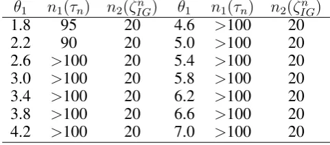
Plot the evolution ofτn and the averaged value of
ζn
IGin Figure 2. In Figure 2, the red curve corresponds
20 40 60 80 100
0.1
0.3
0.5
sample size n
τn
20 40 60 80 100
10
15
20
25
sample size n
ζIG
n
Figure 2: The evolution ofτn(above) and the averaged value of
ζn
IG(blow).
toθ1= 1.8, and the green curve corresponds toθ1= 7. The upper panel in Figure 2 shows that, if the shape parameter θ1 is relatively large, the gamma distribu-tion can be closely approximated by an inverse Gaus-sian distribution. We let n1 denote the sample size, beyond which the value ofτnis smaller than 0.05; let
[image:5.595.41.283.633.752.2]value ofζn
[image:6.595.40.281.104.210.2]IG is larger than 7.815. The evolution ofn1 andn2along with θ1 is summarized in Table 2. From
Table 2: The required sample size for selecting the right model with probability 0.95.
θ1 n1(τn) n2(ζIGn ) θ1 n1(τn) n2(ζIGn )
1.8 95 20 4.6 >100 20
2.2 90 20 5.0 >100 20
2.6 >100 20 5.4 >100 20 3.0 >100 20 5.8 >100 20 3.4 >100 20 6.2 >100 20 3.8 >100 20 6.6 >100 20 4.2 >100 20 7.0 >100 20 Table 2, it is clear that the proposed test statistic is much more efficient thanτn. By comparing Figures 1
and 2 and Tables 1 and 2, it can be found that
• from τn point of view, when fitting a gamma
distribution to inverse-Gaussian distributed data, the probability of selecting the wrong model is small; when fitting an inverse Gaussian distribu-tion to gamma distributed data, the probability of selecting the wrong model is relatively large;
• from ζn
Ga or ζIGn point of view, when fitting
a gamma distribution to inverse-Gaussian dis-tributed data, the required sample size increases with the shape parameterϑ2; when fitting an in-verse Gaussian distribution to gamma distributed data, the required sample size is very small. Because the proposed test statistic is more efficient thanτn, we say that the gamma distribution is more
flexible than the inverse Gaussian distribution.
4 CONCLUSIONS
This paper proposed a test statistic for model selection (or, model-misspecification detection). The gamma process and the inverse Gaussian process were used for illustration, due to their wide applications and essential similarities. Numerical study showed that the proposed approach is more effective than select-ing model based on maximized likelihoods. It was found that the inverse Gaussian density function with a large shape parameter can be well approximated by a gamma density function. The construction of the statistic is based on the Fisher information. Therefore, the statistic is broadly applicable to cases in which the following two qualifications are satisfied.
• The information matrix can be expressed in both the Hessian form and the outer product form.
• The Hessian matrix of the logarithm of the den-sity function is invertible.
REFERENCES
Al Labadi, L. & M. Zarepour (2013). On asymptotic properties and almost sure approximation of the normalized
inverse-gaussian process.Bayesian Analysis 8(3), 553–568.
Dufresne, F., H. U. Gerber, & E. S. W. Shiu (1991). Risk theory
and the gamma process.ASTIN Bulletin 22, 177–192.
Griffin, P. S., R. A. Maller, & D. Roberts (2013). Finite time ruin
probabilities for tempered stable insurance risk processes.
In-surance: Mathematics and Economics 53(2), 478–489. Hyodo, M., T. Yamada, & M. S. Srivastava (2012). A
model selection criterion for discriminant analysis of
high-dimensional data with fewer observations.Journal of
Statis-tical Planning and Inference 142(12), 3134–3145.
Kullback, S. & R. A. Leibler (1951). On information and
suffi-ciency.The Annals of Mathematical Statistics 22(1), 79–86.
Tang, Y., W. Pei, K. Wang, Z. He, & Y. Cheung (2009). A theo-retical analysis of multiscale entropy under the inverse
gaus-sian distribution. International Journal of Bifurcation and
Chaos 19(09), 3161–3168.
Tsai, C., S. Tseng, & N. Balakrishnan (2011). Mis-specification
analyses of gamma and wiener degradation processes.
Jour-nal of Statistical Planning and Inference 141(12), 3725– 3735.
van Noortwijk, J. M. (2009). A survey of the application of
gamma processes in maintenance.Reliability Engineering &
System Safety 94(1), 2–21.
Wasan, M. T. (1968). On an inverse gaussian process.
Scandina-vian Actuarial Journal 1968(1-2), 69–96.
White, H. (1982). Maximum likelihood estimation of
misspeci-fied models.Econometrica 50(1), 1–25.
Zhang, M., Z. Ye, & M. Xie (2014). A condition-based
mainte-nance strategy for heterogeneous populations.Computers &
Industrial Engineering 77, 103 – 114.
Zhang, S. & W. Zhou (2014). Cost-based optimal mainte-nance decisions for corroding natural gas pipelines based on
stochastic degradation models. Engineering Structures 74,
74 – 85.
Zhou, Q. M., P. X. Song, & M. E. Thompson (2012). In-formation ratio test for model misspecification in
quasi-likelihood inference.Journal of the American Statistical
As-sociation 107(497), 205–213.
Zhu, W., M. Fouladirad, & C. Brenguer (2015). Condition-based maintenance policies for a combined wear and shock
deteri-oration model with covariates. Computers & Industrial