Formation of a Convex Structure During the Counter-Rotating Electrochemical Machining of TC4 Titanium Alloy in NaCl Solution

Int. J. Electrochem. Sci., 14 (2019) 9042 – 9057, doi: 10.20964/2019.09.60

International Journal of

ELECTROCHEMICAL

SCIENCE

www.electrochemsci.org

Formation of a Convex Structure During the Counter-Rotating

Electrochemical Machining of TC4 Titanium Alloy in NaCl

Solution

Dengyong Wang1,2,*_{, Wenjian Cao}1,2_{, Bin He}1,2

1 _{College of Mechanical and Electrical Engineering, Nanjing University of Aeronautics and}

Astronautics, Nanjing, China

2 _{Jiangsu Key Laboratory of Precision and Micro-Manufacturing Technology, Nanjing, China} *_{E-mail: [email protected]}

Received: 5 May 2019 / Accepted: 12 July 2019 / Published: 5 August 2019

Because of its outstanding properties, titanium alloy is a very important material in the aerospace industry. However, the machining of titanium alloy poses many challenges for conventional mechanical methods. The aim of the present study is to fabricate a highly convex structure with straight sidewall profiles from TC4 titanium alloy by using counter-rotating electrochemical machining. Neutral NaCl solution is chosen as the working electrolyte on basis of the corrosion morphologies of TC4 alloy at different current densities, and the volumetric electrochemical equivalent of TC4 alloy in NaCl solution is obtained by using weight-loss measurements. Based on an established simulation algorithm flowchart, the evolution of the profile of the convex structure is simulated for different amounts of tool feed. The sidewall taper angle and the amount of stray corrosion on the surface of the convex structure are analyzed. The simulation results show that the taper angle decreases rapidly with the amount of tool feed, and a straight convex structure can be obtained with a suitable amount of tool feed. The amount of stray corrosion on the surface of the convex structure increases constantly because of the linear dissolution characteristic of TC4 alloy in the active NaCl solution. An experiment is also conducted using a specific experimental apparatus. A highly convex structure with a small sidewall taper angle of 3.78° is fabricated successfully on the surface of a cylindrical TC4 workpiece and can be as high as 6.91 mm. The machined surface is smooth with no pitting corrosion, and the profile of the machined convex structure fits well with the simulation result.

Keywords: Electrochemical machining; Counter-rotating; Convex structure; Titanium alloy; Stray corrosion

1. INTRODUCTION

usually has low thermal conductivity, a small coefficient of plastic deformation, and severe strain hardening, all of which lead to serious tool wear and a long processing cycle for conventional mechanical methods [3,4].

As an anodic dissolution process, electrochemical machining (ECM), is efficient at dissolving metal materials without tool wear and machining stress [5-7], and as such it has become a commonly used method for machining titanium alloy. Many previous studies have investigated the anodic dissolution of titanium alloy in ECM conditions. Weinmann et al. investigated the dissolution behavior of Ti90Al6V4 and Ti60Al40 alloys and found that increasing the concentration of chloride ions in the electrolyte could facilitate the dissolution process [8]. Xu et al. studied the electrochemical dissolution behavior of Ti60 alloy and optimized the concentration and temperature of sodium chloride electrolyte in the ECM of a blisk sector [9,10]. Munirathinam et al. studied the electrochemical behavior of titanium in chloride solution of different pH values and analyzed the properties of a thin passive film formed on the surface [11]. Speidel et al. used a doping sodium chloride electrolytes with sodium fluoride to reduce the pitting corrosion during electrolyte jet machining of titanium alloys [12]. Liu et al. investigated the anodic behavior of TB6 titanium alloy in sodium chloride solution [13]. Fushimi et al. examined the anodic dissolution behavior of titanium in chloride-containing ethylene glycol solution [14,15]. Mishra et al. used a mixed solution of sodium nitrate and sodium chloride in the electrochemical milling of Ti6Al4V [16]. He et al. studied the titanium alloy Ti6Al4V in a side-flow electrochemical machining, and the relationship between the feed rate, the processing current, balance gap and surface roughness was analyzed [17].

Herein, we focus on the counter-rotating electrochemical machining (CRECM) of TC4 titanium alloy in NaCl solution. CRECM is a new ECM method proposed by Zhu et al. to machine the complex outer surfaces of revolving parts such as aero-engine casings [18,19]. A cylindrical tool electrode with concave cavities is typically used in CRECM. The anode workpiece and tool electrode rotate in opposite directions at the same angular speed, and the convex structures are fabricated gradually on the corresponding areas of the concave cavities. Previous studies of the CRECM process were concerned mainly with the formation of convex structures on workpieces made of either stainless steel 304 or Inconel 718 [18-21]. The heights of the machined convex structures were no more than 2 mm, and their sidewalls usually had large taper angles.

cylindrical TC4 workpiece. The machined surface is smooth with no pitting corrosion, and the profile of the machined convex structure fits well with the simulation result.

2. ANODIC DISSOLUTION CHARACTERISTICS 2.1 Corrosion morphologies

In ECM, neutral NaNO3 and NaCl solutions are the two most commonly used electrolytes. To

choose a suitable electrolyte, TC4 samples of dimensions 5 mm × 5 mm × 10 mm are corroded electrochemically in 20% NaNO3 solution and 10% NaCl solution at different current densities. The

corrosion time for each experiment is 120 s. Fig. 1 shows the corrosion morphologies of TC4 alloy in the NaNO3 solution, where the quality of the surface of the TC4 alloy is clearly very poor. At low current

densities of up to 10 A/cm2_{, material dissolution occurs only in the marginal areas, and pitting corrosion}

is evident. Upon increasing the current density to 40 A/cm2, the dissolution areas expand but some uncorroded sections remain on the surface. Even at the relatively high current density of 80 A/cm2_{, a}

rough corroded surface can be found, thereby indicating that NaNO3 solution is unsuitable for machining

TC4 alloy.

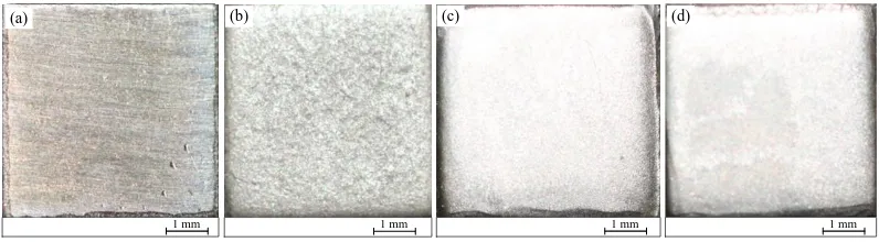
By contrast, Fig. 2 shows that the corrosion morphologies of TC4 alloy in NaCl solution present far better surface quality. Despite the surface being slightly rough at low current densities of up to 10 A/cm2, the material dissolves on the entire surface. Increasing the current density improves the surface roughness remarkably, and a smooth surface is obtained when the current density exceeds 40 A/cm2. Consequently, we choose the NaCl solution as the working electrolyte for TC4 alloy.

Figure 1. Corrosion morphologies of TC4 alloy in 20% NaNO3 solution for 120 s at a current density of

(a) 2 A/cm2, (b) 10 A/cm2, (c) 40 A/cm2, and (d) 80 A/cm2.

Figure 2. Corrosion morphologies of TC4 alloy in 10% NaCl solution for 120 s at a current density of (a) 2 A/cm2, (b) 10 A/cm2, (c) 40 A/cm2, and (d) 80 A/cm2.

1 mm

(a)

1 mm

(b)

1 mm

(c)

1 mm

(d)

1 mm

(a)

1 mm

(b)

1 mm

(c)

1 mm

2.2 Volumetric electrochemical equivalent

The anodic dissolution rate v (cm/min) in ECM is determined mainly by the VEE ω of the material and the current density i and can be calculated using Faraday’s Law [22-26], namely



=

v i (1)

where η is the current efficiency which is equals to 100% in the active NaCl solution.

The VEE ω is essential for predicting the anode shaping process in ECM, which depends strongly on the metal composition:

1 2 1 2 1 2 1 ( )   =

+ + + j

j j

n

n n

F a a a

A A A

(2)

where ρ is the density of metal, F is the Faraday constant, nj is the valence of dissolution, Aj is the atomic

weight of the dissolving atoms type, and aj is the element content.

Previous studies focused on other metals such as stainless steel 304, Inconel 718, and annealed steel 100 Cr6 in NaNO3 solution [27,28]. However, the VEE for TC4 alloy in 10% NaCl solution is yet

to be reported. For TC4 alloy, apart from the main metal components of Ti, Al, and V as listed in Table 1, there are also some impurity elements such as Fe, C and O. It is therefore difficult to calculate the VEE accurately using the theoretical formula. To obtain the VEE ω of TC4 in NaCl solution, the TC4 specimens were dissolved at different current densities. The machining current I and the dissolution time t in each test were controlled to be constant, and the specimens were weighed precisely before and after each experiment. The VEE ω can be calculated as:

M It 





= (3)

where ΔM is the amount of metal dissolution in each test.

Table 1. Main metal components of TC4 alloy.

Element Ti Al V

wt% Balance 5.9 6.7

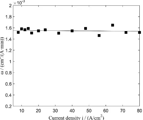
Fig.3 shows the measured VEE ω of TC4 alloy in 10% NaCl solution, from which ω is independent of the current density i in the active NaCl solution. Despite some fluctuations due to measurement errors, ω can be determined to be a constant at 0.0015 cm3_{/ (A·min). This means that the}

Figure 3. Measured volumetric electrochemical equivalent ω of TC4 alloy in 10% NaCl solution.

3. NUMERICAL SIMULATION 3.1 Simulation procedure

Fig. 4 shows the principle of using CRECM to form a convex structure on the surface of a cylindrical workpiece [20]. The workpiece is used as the anode, a cylindrical tool electrode with a concave cavity is used as the cathode. The workpiece and tool electrode rotate in opposite directions at the same rotation speed while the tool electrode is fed toward the workpiece at a constant feed rate. The NaCl electrolyte flows into the inter-electrode gap from one side of the electrodes and flows out from the other side. When a certain direct voltage is applied between the anode workpiece and tool electrode, the materials on the anode surface are dissolved during the rotation of the electrodes. Because of the existence of the concave cavity on the tool electrode, the corresponding area on the workpiece remains as a convex structure.

w w

Anode workpiece

Tool electrode

f

Electrolyte flow

Electrolyte flow

M

Mx

My

P

x y

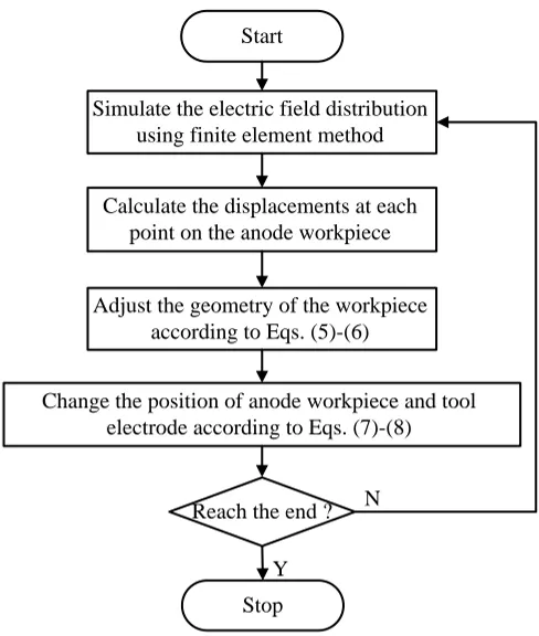
To simulate the process of forming a convex structure in CRECM, the machining process is discretized into a series of short time periods. Fig. 5 shows the simulation procedure as a flowchart. During each short time period, the electric field within the inter-electrode gap is calculated by using the finite element method, and the current density at each point on the anode surface is obtained according to

x x

i =E (4)

y y

i =E (5)

where ix and iy are the current densities in x and y directions, repectively, κ is the electrolyte conductivity,

and Ex and Ey are the electric field intensities in the x and y directions, repectively.

The amount of material dissolution in one time period can be calculated according to Eq. (1), and the displacements for point P (Fig. 4) on the anode workpiece are described as

 

=  = 

x x x

M i t E t (6)

 

=  = 

y y y

M i t E t (7)

where Mx and My are the displacements in the x and y directions, repectively, and Δt is the duration of

each step.

Start

Simulate the electric field distribution using finite element method

Calculate the displacements at each point on the anode workpiece

Adjust the geometry of the workpiece according to Eqs. (5)-(6)

Change the position of anode workpiece and tool electrode according to Eqs. (7)-(8)

Reach the end ?

Stop

N

Y

Figure 4. Algorithm flowchart of simulation procedure.

In the next time period, the workpiece and tool electrode rotate oppositely by a small angle Δφ, and the tool electrode moves towards the workpiece by a certain distance Δd. The rotation angle Δφ and the feed distance Δd satisfy

w t 

d f t

 =  (9)

where w is the angular speed and f is the tool feed rate.

The electric field distribution and the displacements at each point on the anode workpiece are then calculated again. Through thousands of calculation cycles, the final profile of the convex structure is simulated under the conditions listed in Table 2.

The simulation conditions are listed in table 2.

Table 2. Simulation conditions.

Parameters Value

Diameter of the workpiece Φ50 mm

Diameter of the tool electrode Φ50 mm

Width of the concave cavity 18 mm

Applied voltage U 30V

Electrolyte concentration 10% NaCl

Volumetric electrochemical equivalents ω 0.0015 cm3_{/ (A·min)}

Angular velocity w 2π rad/min

Tool feed rate f 0.1 mm/min

Tool feed amount F 9 mm

3.2 Evolution of shape of the convex structure

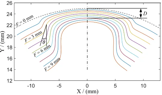
Fig. 6 shows the simulated evolution of the profile of the convex structure for different amounts of tool feed. The convex structure forms gradually on the surface of the anode workpiece. When the amount of tool feed is 1 mm, the convex structure is machined to be around 1 mm tall and 16.53 mm wide. With the amount of tool feed increases, the convex structure becomes taller and narrower. When the amount of tool feed is 9 mm, the convex structure grows in height to around 7.14 mm and shrinks in width to around 9.4 mm. Compared with the initial contour of the workpiece (the dashed line), the top outline of the simulated convex structure moves downward with the amount of tool feed. This is due to the existence of stray corrosion on the surface of the convex structure, which is caused by the poor localization effect of the anodic dissolution of TC4 alloy in the active NaCl solution (Fig. 3). In particular, the simulated profiles show that the sidewall of the convex structure becomes straighter with increasing height.

In all the previous studies, the convex structures machined by CRECM on stainless steel 304 and Inconel 718 workpieces were no more than 2 mm tall, and their sidewall profiles were tapered [18–21]. Consequently, to machine a convex structure with small taper angle on TC4 alloy in NaCl solution, we analyze the variation tendencies of the sidewall taper angle and the height of the convex structure.

θ

F = 0 m m

F = 3 m m

F = 6 m

m

F = 9

mm

D

X / (mm)

Y

/

(

m

m

)

Figure 6. Simulated shape evolution of convex structure for different amounts of tool feed.

3.3 Variation of sidewall taper angle of convex structure

To better reflect the variation tendency of the sidewall profile, we consider the taper angle θ for different amounts of tool feed. Fig. 7 shows the taper angles measured at different amounts of tool feed, where the taper angle reaches 32.6° for 1 mm of the tool feed and then the taper angle decreases rapidly with the amount of tool feed. For 9 mm of tool feed, the measured taper angle is only -0.49°, which indicates a favorable straight sidewall profile. The fitting curve of the taper angle shows a cubic relationship between the taper angle θ and the amount F of tool feed, namely

 = −_0.0411F3+_1.07F2−_11.1F+_42.7

(10)

According to Eq. (7), to obtain a straight convex structure, the corresponding theoretical amount F of tool feed should be 8.73 mm.

3.4 Variation of height of convex structure

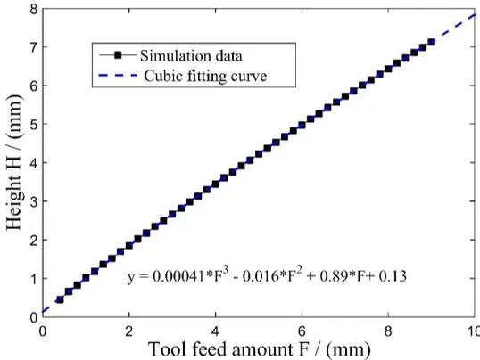
The height of the convex structure is determined mainly by the amounts of tool feed and stray corrosion on the surface. Based on the simulation results in Fig. 6, the amount D of stray corrosion at the peak of the convex structure was measured and is plotted in Fig. 8. The amount D of stray corrosion rises rapidly with the amount F of tool feed, with D reaching 2.39 mm at F = 9 mm. The variation of the amount D of stray corrosion is descried using the cubic fitting equation

3 2

0.000315 0.00224 0.22 0.00298

= + + −

D F F F (11)

Figure 8. Amount of stray corrosion on the surface of convex structure for different amounts of cathode feed.

Figure 9. Height of convex structure for different amounts of cathode feed.

where H reaches 7.14 mm at F = 9 mm. The rising tendency of the height also satisfies a cubic fitting curve, namely

(12)

3.5 Relationship between sidewall taper angle and height of convex structure

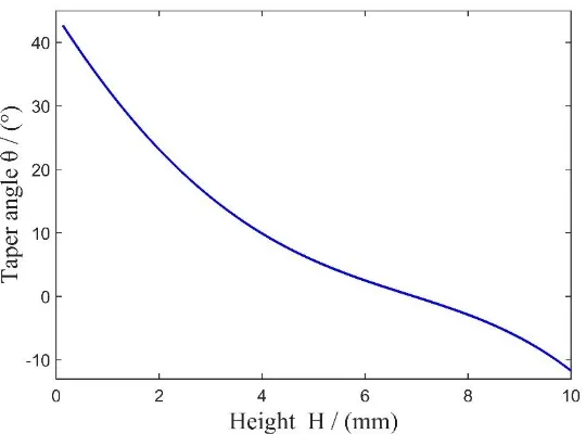
Based on Eqs. (7) and (8), the relationship between the sidewall taper angle θ and the height H can be obtained. The variational tendency is shown in Fig. 10, where the sidewall taper angle exceeds 40° initially and then decreases rapidly with the height of the convex structure. In particular, when H ≈ 6.95 mm, we have θ ≈ 0, after which the taper angle becomes negative. When H reaches 10 mm, the negative taper angle reaches −11.7°.

Figure 10. Variation of sidewall taper angle with height of convex structure.

4. EXPERIMENTAL RESULTS AND DISCUSSION

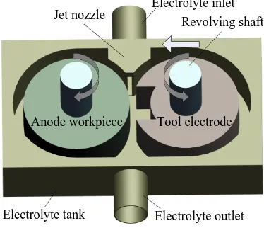
A specific experimental apparatus was developed to access the effectiveness of the simulation of the convex shaping process in CRECM [29,30]. As shown in Fig. 11, the cylindrical workpiece and tool electrode were mounted on two synchronous revolving shafts, and the tool electrode could move simultaneously along the center line. Both the workpiece and tool electrode were immersed in an enclosed tank, and the NaCl electrolyte was pumped out from the jet nozzle. The pressure of the electrolyte was 0.2 MPa, and the temperature was controlled to be 30℃. The applied voltage is 30 V, and the angular rotation speed was 2π rad/min. The feed rate of the tool electrode was 0.1 mm/min, and the total amount of tool feed was 9 mm. Fig. 12 shows a photograph of the fabricated tool electrode with a concave cavity. To shield the electric field, the sidewalls of the cavity were coated with a ceramic insulator layer.

3 2

0.00041 0.016 0.89 0.13

= +

Electrolyte inlet

Electrolyte outlet Jet nozzle

Electrolyte tank

Revolving shaft

Anode workpiece Tool electrode

Figure 11. Schematic of experimental apparatus.

Ceramic insulator layer

Figure 12. Photograph of tool electrode with concave cavity.

10 mm 5 mm

(a) (b)

Figure 13. (a) Photograph of machined TC4 workpiece; (b) Enlarged view of convex structure.

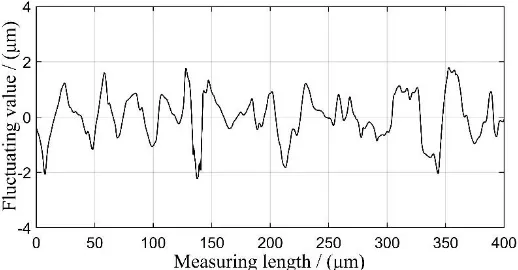
Figure 14. Surface roughness measured using a 3D optical profiler.

3.78°

R2.5

R4.2

D

α

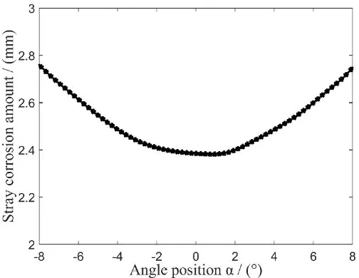
Figure 16. Amounts of stray corrosion on the top surface of the machined convex structure.

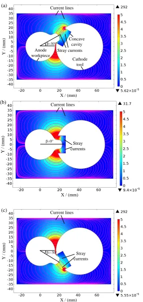
To better illustrate the occurrence of stray corrosion on the surface of convex structure, the electric field within the electrolyte domain is simulated on basis of COMSOL software [31,32]. Fig. 17 shows the current density distributions within the inter-electrode gap at different rotation angles. The red areas have a high current density ≥ 5 A/cm2_{, and blue areas have a low current density ≤ 1 A/cm}2_{. The}

magenta lines represent the machining currents. It is seen that although the current densities on the surface of the convex structure are much smaller than that in the machining area, stray currents can still been observed for each rotation angle, which travel from the surface of convex structure to the edges of the concave cavity.

The current densities on the surface of convex structure are extracted and plotted in Fig. 18. The horizontal ordinate is the arc length of the convex surface, and its origin is set at the center of the convex structure. For rotation angle β = -30° and 30°, remarkable stray current densities ranging from around 1.3 A/cm2 to 4 A/cm2 can be found on the surface of the convex structure. For rotation angle β = 0°, the stray current density on both sides can be as high as 3.7 A/cm2_{. Even at the center area, the minium stray}

Concave cavity Stray currents Current lines

X / (mm)

Y

/

(

m

m

)

β=30°

(a)

Anode workpiece

Cathode tool

Stray currents Current lines

X / (mm)

Y

/

(

m

m

)

β=0°

(b)

Stray currents Current lines

X / (mm)

Y

/

(

m

m

)

β=-30°

(c)

Figure 18. Stray current densities on the top surface of the machined convex structure at different rotation angles.

5. CONCLUSIONS

In this paper, the process of forming a convex structure during the CRECM of TC4 alloy in NaCl solution was investigated. The conclusions are summarized as follows:

(1) The corrosion morphologies of TC4 alloy at different current densities indicated that using NaNO3 solution would lead to poor machined surfaces. By contrast, smooth surfaces could be obtained

by using NaCl solution.

(2) The VEE of TC4 alloy in NaCl solution was determined to be a constant value of 0.0015 cm3_/

(A·min) on basis of weight-loss measurements.

(3) The profile evolution of the convex structure was simulated at different amounts of tool feed. The variation tendencies of the sidewall taper angle and the height of the convex structure were analyzed. The results indicated that a highly convex structure with straight sidewalls can be obtained by choosing a suitable amount of tool feed.

(4) A convex structure with a small sidewall taper angle of 3.78 °was fabricated successfully by using a tool electrode with a concave cavity. The convex structure can be as high as 6.91 mm, the machined surface was smooth with no pitting corrosion, and the profile of the machined workpiece fits well with the simulation result.

ACKNOWLEDGEMENTS

References

1. M. Peters, J. Kumpfert, C.H. Ward and C. Leyens, Adv. Eng. Mater., 5 (2003) 419. 2. R.R. Boyer and R.D.Briggs, J. Mater. Eng. Perform., 14 (2005) 681.

3. E.O. Ezugwu and Z.M. Wang, J. Mater. Process. Tech., 68 (1997) 262. 4. M. Rahman, W.Y. San, Z.A. Rahmath, Jsme Int. J., 46 (2003) 107.

5. K.P. Rajurkar, D. Zhu, J.A. Mcgeough, J. Kozak and A. DeSilva, CIRP Ann., 44 (1999) 567. 6. R.R. Venkata and V.D. Kalyankar, Int. J. Adv. Manuf. Technol., 73 (2014) 1159.

7. K.P. Rajurkar, M.M. Sundaram, A.P. Malshe, Proc. CIRP, 6 (2013) 13.

8. M. Weinmann, M. Stolpe, O. Weber, R. Busch and H. Natter, J. Solid State Electr., 19 (2015) 485. 9. Z.Y. Xu, X.Z. Chen, Z.S. Zhou, P. Qin and D. Zhu, Proc. CIRP, 42 (2016) 125.

10.X.Z. Chen, Z.Y. Xu, D. Zhu, Z.D. Fang and D. Zhu, Chinese J. Aeronaut., 29 (2016) 274. 11.B. Munirathinam, R. Narayanan and L. Neelakantan, Thin Solid Films, 598 (2016) 260.

12.A. Speidel, J. Mitchell-Smith, D.A. Walsh, M. Hirsch and A. Clare, Proc. CIRP, 42 (2016) 367. 13.W.D. Liu, S.S. Ao, Y. Li, Z.M. Liu, H. Zhang, S. Marwana Manladan, Z. Luo and Z.P. Wang,

Electrochim. Acta, 233 (2017) 190.

14.K. Fushimi, H. Kondo and H. Konno, Electrochim. Acta, 55 (2009) 258. 15.K. Fushimi and H. Habazaki, Electrochim. Acta, 53 (2008) 3371.

16.K. Mishra, D. Dey, B.R. Sarkar and B. Bhattacharyya, J. Manuf. Process., 29 (2017) 113.

17.Y.F. He, J.S. Zhao, H.X. Xiao, W.Z. Lu and W.M. Gan, Int. J. Electrochem. Sci., 13 (2018) 5736. 18.Z.W. Zhu, D.Y. Wang, J. Bao, N.F. Wang and D. Zhu, Int. J. Adv. Manuf. Technol., 80 (2015) 1957. 19.D.Y. Wang, Z.W. Zhu, B. He, D. Zhu and Z.D. Fang, J. Manuf. Process., 35 (2018) 614.

20.D.Y. Wang, Z.W. Zhu, H.R. Wang and D. Zhu, Chinese J. Aeronaut., 29 (2016) 534. 21.D.Y. Wang, B. He, Z.W. Zhu, Y.C. Ge and D. Zhu, J. Electrochem. Soc., 165 (2018) 282. 22.N.S. Qu, X.L. Fang, W. Li, Y.B. Zeng and D. Zhu, Chinese J. Aeronaut., 26 (2013) 224. 23.T. Paczkowski and J. Sawicki, Mach. SCI. Technol., 12 (2016) 33.

24.D. Zhu, N.S. Qu, H.S. Li, Y.B. Zeng, D.L. Li and S.Q. Qian, CIRP Ann., 58 (2009) 177.

25.V.P. Zhitnikov, N.M. Sherykhalina and A.A. Zaripov, J. Mater. Process. Technol., 235 (2016) 49. 26.H.S. Li, C.P. Gao, G.Q. Wang, N.S. Qu and D. Zhu, Sci. Rep., 6 (2016) 35013.

27.D.Y. Wang, Z.W. Zhu, N.F. Wang, D. Zhu and H.R. Wang, Electrochim. Acta, 156 (2015) 301. 28.T. Haisch, E. Mittemeijer and J.W. Schultze, Electrochim. Acta, 47 (2001) 235.

29.Y.C. Ge, Z.W. Zhu, D. Zhu and D.Y. Wang, Chinese J. Aeronaut., 31 (2018) 2049. 30. D.Y. Wang, Z.W. Zhu, J. Bao and D. Zhu, Int. J. Adv. Manuf. Technol., 76 (2015) 1365.