Q rung orthopair normal fuzzy aggregation operators and their application in multi attribute decision making

Article

Q-rung Orthopair Normal Fuzzy Aggregation

Operators and Their Application in

Multi-Attribute Decision-Making

Zaoli Yang1_{, Xin Li}1_{, Zehong Cao}2_{and Jinqiu Li}3,_*

1 _{College of Economics and Management, Beijing University of Technology, Beijing 100124, China;}

[email protected] (Z.Y.); [email protected] (X.L.)

2 _{Discipline of ICT, School of Technology, Environments and Design, College of Sciences and Engineering,}

University of Tasmania, Hobart, TAS 7001, Australia; [email protected]

3 _{College of Economics and Management, Harbin Engineering University, Harbin 150001, China}

* Correspondence: [email protected] or [email protected]; Tel.:+86-1563-606-6885

Received: 6 November 2019; Accepted: 20 November 2019; Published: 22 November 2019

Abstract:Q-rung orthopair fuzzy set (q-ROFS) is a powerful tool to describe uncertain information in the process of subjective decision-making, but not express vast objective phenomenons that obey normal distribution. For this situation, by combining the q-ROFS with the normal fuzzy number, we proposed a new concept of q-rung orthopair normal fuzzy (q-RONF) set. Firstly, we defined the conception, the operational laws, score function, and accuracy function of q-RONF set. Secondly, we presented some new aggregation operators to aggregate the q-RONF information, including the q-RONF weighted operators, the q-RONF ordered weighted operators, the q-RONF hybrid operator, and the generalized form of these operators. Furthermore, we discussed some desirable properties of the above operators, such as monotonicity, commutativity, and idempotency. Meanwhile, we applied the proposed operators to the multi-attribute decision-making (MADM) problem and established a novel MADM method. Finally, the proposed MADM method was applied in a numerical example on enterprise partner selection, the numerical result showed the proposed method can effectively handle the objective phenomena with obeying normal distribution and complicated fuzzy information, and has high practicality. The results of comparative and sensitive analysis indicated that our proposed method based on q-RONF aggregation operators over existing methods have stronger information aggregation ability, and are more suitable and flexible for MADM problems.

Keywords: normal fuzzy number; Q-rung orthopair normal fuzzy sets; q-RONF information aggregation operators; multi-attribute decision-making

1. Introduction

On the basis of Zadeh’s fuzzy sets [1], Atanassov [2] proposed intuitionistic fuzzy sets (IFS) to characterize the uncertainty according to membership degree (MED) and non-membership degree (NOMED). IFS made up for the insufficiency that Zadeh’s fuzzy sets can only characterize fuzzy information by MED. IFS have attracted extensive attention of many scholars who further expanded the IFS, such as interval IFS [3,4], 2-tuple IFS [5], trapezoidal IFS [6,7], intuitionistic normal fuzzy sets [8], intuitionistic uncertain linguistic [9], triangular IFS [10,11], etc. IFS requires that the sum of MED and NOMED is not more than 1, and this restricts its application in practical decision-making problems. For example, when decision makers (DMs) independently give the MED and NOMED of one attribute of the alternative, the sum of the them may be greater than 1, and their quadratic sum will be less than or equal to 1. At the same time, Yager pointed out a situation, with an example [12], when the MED given by the DM is

√

3/2, and NOMED is 1/2, then √

3/2+1/2>1, but( √

3/2)2_{+ (1/2)}2_≤

1

( √

3/2)2+ (1/2)2 ≤ _{1. For this situation, Yager [12,13] proposed Pythagorean fuzzy sets (PFS),} whose characteristic is that the quadratic sum of MED and NOMED is not greater than 1. Compared with IFS, the PFS characterizes fuzzy information more effectively. Since PFS was proposed, many scholars have conducted in-depth studies [13–23].

Although IFS and PFS have been extensively studied, their expression for fuzzy information is still limited, especially in the extremely complex and contradictory information environment. When the quadratic sum of MED and NOMED given by DMs is still greater than 1, but the sum of three or higher powers is less than 1, IFS and PFS can not deal with such type of information. In order to compensate for the deficiencies of IFS and PFS, and enhance the ability of characterizing fuzzy information. Yager [24] further proposed the concept of q-rung orthopair fuzzy set (q-ROFS) whose characteristics are that the sum of q power of MED and NOMED is bound to 1, when q>1, and that when q=1 and 2, q-ROFS becomes IFS and PFS, respectively. Many scholars have carried out extensive research and discussion on the concept of q-ROFS as following three aspects: (1) In terms of basic theory, some studies analyzed some properties of q-rung orthopair fuzzy (q-ROF) functions [25–28], established the distance measure and similarity measure between q-ROFSs [29,30], and defined some new concepts based on q-ROFS [31,32]. (2) In terms of information aggregation operators, some authors established various types of information aggregation operators based on classic operators under q-ROF environment. Such as the family the q-ROF power aggregation operators [33], a series of q-ROF linguistic aggregation operators [34,35], the family of q-ROF Muirhead mean operators [36,37] a sequence of q-ROF Hamy mean operators [38]. In addition, the ROF information aggregation operators based on Archimedean Muirhead mean operators [39], Bonferroni mean operator [40], Heronian mean operator [41–43], and Choquet integral operator [44] were also developed. (3) In terms of the decision-making method, the existing studies combined the q-ROFS with preference relation [45], distance measure [46], and the TOPSIS method [47,48] to develop the corresponding multi-attribute decision-making method.

In real life, a large number of natural and social phenomenon obey normal distribution [8,49], such as “product life span”, “stock price”, "commodity customer experience evaluation" and so on. In view of these phenomenon, Yang and Ko [49] proposed normal fuzzy number (NFN) to characterize them. Li and Liu [50] pointed out that compared with triangular and trapezoidal fuzzy numbers, NFN has higher derivative continuity, which can characterize natural and social phenomenon more extensively, and their membership functions are closer to human thinking. Li and Liu [50] used examples to prove that the extension of intuitionistic fuzzy number (IFN) based on NFN is better than IFN based on triangular, trapezoidal fuzzy numbers, etc. Therefore, Wang et al. [8] and Wang et al. [51] defined intuitionistic normal fuzzy (INF) number and its operation rules and some information aggregators. Based on these, the concept of interval-valued INF was defined [52], and the family of INF-induced ordered operators [53], and a series of aggregation operators based on classic operators under INF information environment were proposed [54–58].

In summary, PFS and IFS are special cases of q-rung orthopair fuzzy sets. The fuzzy information characterized by q-ROFs is broader and more comprehensive. NIF is closer to human decision-making thinking than triangular and trapezoidal fuzzy numbers. PFS and IFS based on triangular and trapezoidal fuzzy numbers have been reported successively. However, q-rung orthopair fuzzy sets based on INF have not been proposed yet.

In this paper, we defined q-rung orthopair normal fuzzy number, and its operational laws and some aggregation operators, as well as a multi-attribute decision-making method based on q-ROFs algorithm and information aggregator. The rest of this paper is arranged as follows: In Section2, the basic concepts of NFN and q-ROFs are reviewed. In Section3, q-RONFN and some of its operational rules are defined. In Section4, some information aggregation operators in q-RONFs environment are proposed. In Section5, a multi-attribute decision-making method based on q-RONF Information Aggregation operator is proposed. In Section6, an example is given to prove the effectiveness of the

2. Preliminaries

2.1. The Normal Fuzzy Number

Definition 1. ([49])Let R be a real number set, the membership function of

e

A(x) =e−(x −_α

σ )2(σ >0) (1)

is called as a normal fuzzy number (NFN)Ae= (α,σ), the normal fuzzy number set (NFNS) is denoted byNe.

Lemma 1.([59])LetAe,eB∈N, denoted bye Ae= (α,σ),eB= (β,τ), then

(1) λAe=λ(α,σ) = (λα,λσ),λ >0,

(2) Ae+eB= (α,σ) + (β,τ) = (α+β,σ+τ).

Definition 2. ([59])LetAe,eB∈N, denoted bye Ae= (α,σ),eB= (α,σ), then the distance betweenA ande eB can

be defined as

d2Ae,eB

= (α−β₎2₊1 2(σ−τ)

2

. (2)

2.2. The Q-rung Orthopair Fuzzy Number

Definition 3. ([24])Let X be an ordinary fixed set, a q-rung orthopair fuzzy set (q-ROFS) A in X defined by A=n

x,uA(x),vA(x)

x∈X

o

, where uA(x)and vA(x)represent the MED and NOMED, respectively, and uA(x)∈[0, 1], vA(x)∈[0, 1], and0≤uA(x)q+vA(x)q ≤1 (q≥1). The degree of indeterminacy is given as

πA(x) = (uA(x)q+vA(x)q−uA(x)qvA(x)q)1/q. To simplify the expression, a q-rung orthopair fuzzy number (q-ROFN) can be denoted as A= (uA,vA).

Compared with the IFS and PFS, the q-ROFS depicts fuzzy information more broadly. For example, let a fuzzy number be A = h_{0.7, 0.8}i_{, the sum of MED and NOMED of A is 1.5, that exceeds 1,} the quadratic sum of them is 1.13, also more than 1, so the IFS and PFS cannot addressA. However, the sum of 3 power of MED and NOMED is less than 1, hence, we can use q-ROFS to calculateAwith making the parameterq=3 in q-ROFS.

Definition 4.([60])Let a1= (u1,v1)and a2= (u2,v2)be two q-ROFNs,λbe a non-negative real number, then

(1) a1⊕a2=

uq₁+uq₂−_uq 1u

q

2

1/q

,v1v2

,

(2) a1⊗a2=

u1u2,

vq₁+vq₂−_vq 1v

q

2

1/q

,

(3) λa1=

1−₍₁−_uq 1)

λ1/q

,vλ₁

!

,

(4) aλ₁ = uλ₁,

1−₍₁−_vq 1)

λ1/q!

.

Definition 5.([60])Let a= (ua,va)be a q-ROFN, then the score function of a is defined as S(a) =uqa−v q

a,

the accuracy function of a is defined as H(a) = uqa+v q

a. For any two q-ROFNs, a1 = (u1,v1) and a2= (u2,v2), then

(2)If S(a1) =S(a2), then If H(a1)>H(a2), thena1>a2; If H(a1) =H(a2), then a1=a2.

3. The Q-rung Orthopair Normal Fuzzy Number and Its Operations

Based on the notions and operations of q-ROFN and NFN, we presented the q-rung orthopair normal fuzzy number (q-RONFN) and its operations.

Definition 6. Let X be an ordinary fixed non-empty set and(α,σ) ∈N, Ae =(α,σ),(ua,va)is a q-rung orthopair normal fuzzy set (q-RONFS), when its membership function is defined as

uA(x) =uAe

−₍x−α

σ )2_{, x}∈_{X (3)}

and non- membership function is defined as

vA(x) =1−(1−vA)e

−₍x−α

σ )2_{, x}∈_{X, (4)}

where0≤_uA(x),vA(x)≤_1,0≤(uA(x))q+ (vA(x))q≤1, (q≥1). When uA=1and vA=0, the q-RONFS will be transformed into a normal fuzzy number. To simplify the expression, a q-rung orthopair normal fuzzy number (q-RONFN) is denoted as A=

(α,σ),(uA,vA).

Definition 7.Let a1=(α1,σ1),(u1,v1)and a2=(α2,σ2),(u2,v2)be any two q-RONFNs, andλbe a nonnegative real number, then

(1) a1⊕a2=

(α₁+α2,σ1+σ2),

uq₁+uq₂−_uq 1u

q

2

1/q

,v1v2

,

(2) a1⊗a2=

(α1α2,σ1σ2),u1u2,

vq₁+vq₂−_vq 1v

q

2

1/q

,

(3) λa1= (λα1,λσ1),

1−₍₁−_uq 1)

λ1/q

,vλ₁

!

,

(4) aλ₁ = αλ₁,σλ₁,uλ₁,

1−₍₁−_vq 1)

λ1/q!

.

Proposition 1. Let a1 =(α1,σ1),(u1,v1), a2= (α2,σ2),(u2,v2)and a3 =(α3,σ3),(u3,v3)be any three q-RONFNs, andλ,λ1,λ2be nonnegative real numbers, we can obtain that

(1) a1+a2=a2+a1,

(2) (a1+a2) +a3=a1+ (a2+a3),

(3) a1×a2=a2×a1,

(4) (a1×a2)×a3=a1×(a2×a3),

(5) λ1a1+λ2a1= (λ1+λ2)a1,

(6) λ(a1+a2) =λa1+λa2,

(7) aλ1₁ λ2 =aλ1λ2₁ .

Proof.According to the Definition 7, we can easily infer that (1), (3), (5), (6) and (7) are obviously right, (2) and (4) need be proved as follows:

For (2)(a1+a2) +a3=a1+ (a2+a3).

Let the NFN of q-RONFNrbeNer, the MED of(a₁+a₂) +a₃ anda₁+ (a₂+a₃)beu_(a

1+a2)+a3

andua1+(a2+a3), and the NOMED of(a1+a2) +a3 anda1+ (a2+a3)bev(a1+a2)+a3 andva1+(a2+a3),

respectively, and we can obtain that

e

N_(r1+r2)+r3=Ne_r

u_(a1+a2)+a3 =uq₁+uq₂−_uq 1u

q

2+u

q

3−(u

q

1+u

q

2−u

q

1u

q

2)u

q

3

1/q

=uq₁+uq₂+uq₃−_uq 1u

q

2−u

q

1u

q

3−u

q

2u

q

3+u

q

1u

q

2u

q

3

1/q

ua1+(a2+a3)=

uq₂+uq₃−_uq 2u

q

3+u

q

1−(u

q

2+u

q

3−u

q

2u

q

3)u

q

1

1/q

=uq₁+uq₂+uq₃−_uq 1u

q

2−u

q

1u

q

3−u

q

2u

q

3+u

q

1u

q

2u

q

3

1/q

u(a1+a2)+a3 =ua1+(a2+a3).

Similarly, we can get thatv(a1+a2)+a3 =va1+(a2+a3).

Therefore,(a1+a2) +a3=a1+ (a2+a3).

For (4)(a1×a2)×a3=a1×(a2×a3).

Let the normal fuzzy number of q-RONFNsrbeNer, the MED of(a₁×a₂)×a₃anda₁×(a₂×a₃)

beu(a1×a2)×a3 andua1×(a2×a3), and the NOMED of (a1×a2)×a3 anda1×(a2×a3)bev(a1×a2)×a3 and va₁×_(a2×_a3), respectively, and we can obtain that

e

N_(r1×_r2)×_r3=Ne_r

1×(r2×r3)= (α1×α2×α3,σ1×σ2×σ3),,

v(a1×a2)×a3 =

vq₁+vq₂−_vq 1v

q

2+v

q

3−(v

q

1+v

q

2−v

q

1v

q

2)v

q

3

=vq₁+vq₂+vq₃−_vq 1v

q

2−v

q

1v

q

3−v

q

2v

q

3+v

q

1v

q

2v

q

3

v(a1×a2)×a3 =

vq₂+vq₃−_vq 2v

q

3+v

q

1−(v

q

2+v

q

3−v

q

2v

q

3)v

q

1

=vq₁+vq₂+vq₃−_vq 1v

q

2−v

q

1v

q

3−v

q

2v

q

3+v

q

1v

q

2v

q

3

v(a₁×_a2)×_a3 =v_a

1×(a2×a3).

Similarly, we can get thatu(a1×a2)×a3 =ua1×(a2×a3).

Definition 8. Let a=

(α,σ),(u,v)

be a q-RONFN, its score function is defined as

S1(a) =α

uqa−v q a

,S2(a) =σ

uqa−v q a

,

its accuracy function is defined as

H1(a) =α

uq_a+vq_a,H2(a) =σ

uq_a+vq_a.

Definition 9. Let a1 = (α1,σ1),(u1,v1), a2 = (α2,σ2),(u2,v2) be any two q-RONFNs, their score functions are S1(a), S2(a), their accuracy functions are H1(a), H2(a), respectively, then we can get

(1)If S1(a1)>S1(a2), then a1>a2,

(2)If S1(a1) =S1(a2)and H1(a1)>H1(a2),then a1>a2,

(3)If S1(a1) =S1(a2)and H1(a1) =H1(a2), If S2(a1)<S2(a2), then a1>a2,

If S2(a1) =S2(a2)and H2(a1)<H2(a2), then a1>a2, If S2(a1) =S2(a2)and H2(a1) =H2(a2), then a1=a2.

4. Q-Rung Orthopair Normal Fuzzy Aggregation Operators

Based on operational rules of q-RONFN, we will present some q-Rung orthopair normal fuzzy (q-RONF) aggregation operators.

4.1. The q-RONF Weighted Aggregation Operators

Definition 10. Let ai = (αi,σi),(ui,vi) (i = 1, 2,· · ·,n)be a collection of the q-RONFNs, and w = (w1,w2,· · · ,wn)Tbe the weight vector of ai, and0≤wi ≤1 (i=1, 2,· · ·,n)T,Pni=1wi =1, then

q−_{RONFWA(a1,a2,}· · · _{,an) =} n

X

i=1

wiai (5)

is called an q-RONF weighted averaging (q-RONFWA) operator.

Theorem 1. Let ai=(αi,σi),(ui,vi)(i=1, 2,· · · ,n)be a collection of the q-RONFNs, the value by using Definition 10 is still a q-RONFN, that is

q−_{RONFWA(a1,a2,}· · ·_{,an) =}

*

( n

X

i=1

wiαi, n

X

i=1

wiσi),



       

     

1− n

Y

i=1

1−_uq i

wi



     

1/q

, n

Y

i=1

vwi i



       +

. (6)

Proof.The mathematical induction method is used to prove the Theorem 1 as follows: (1) Whenn=2,

Since

w1a1=

(w1α1,w1σ1),

1−₁−_uq 1

w11/q

,vw1 1

,

and

w2a2=

(w2α2,w2σ2),

1−₁−_uq 2

w₂1/q

,vw2 2

,

then

q−_{RONFWA(a1,a2) =w1}α₁⊕_w2α₂

=

*

(w1α1+w2α2,w1σ1+w2σ2),

                      

1−₁−_uq 1

w11/qq

+

1−₁−_uq 2

w21/qq

−

1−₁−_uq 1

w₁1/qq

1−₁−_uq 2

w21/qq

          

1/q

,vw1 1 v

w2

2

           

+

=

* (

2

P

i=1

wiαi,

2

P

i=1

wiσi),

1−₁−_uq 1

w1

+1−₁−_uq 2

w2

−₁−₁−_uq 1

w1

1−₁−_uq 2

w21/q

,

2

Q

i=1

vwi i

! +

=

*

( 2

P

i=1

wiαi,

2

P

i=1

wiσi),

    

 1

− 2

P

i=1

1−_uq i

wi!1/

q ,

2

Q

i=1

vwi i

      +

(2) Supposingn=k, k>2, that is

q−_RONFWA(a1,a2,· · ·,ak) =

*

( k

X

i=1

wiαi, k

X

i=1

wiσi),

               

1− k

Y

i=1

1−_uq i

wi

      

1/q

, k

Y

i=1

vwi i

         +

Ifn=k+1, according to the operational laws of q-RONFN, we can get

q−_{RONFWA(a1,a2,}· · ·_{,ak,ak+1) =q}−_{RONFWA(a1,a2,}· · ·_,ak)⊕_wk+1α_k+1

=

*

k

P

i=1

wiαi+wk+1αk+1,

k

P

i=1

wiσi+wk+1σk+1

! ,                                              1− k Q

i=1

1−_uq i

wi

!1/q       q +

1−₁−_uq

k+1

wk+11/qq

−       

1−Qk

i=1

1−_uq i

wi

!1/q       q

1−₁−_uq

k+1

wk+11/qq

                  1/q , k Q

i=1

vwi

i v

wk+1

k+1

                    + = *

k+1

P

i=1

wiαi,

k+1

P

i=1

wiσi

! ,               1− k Q

i=1

1−_uq i

w_i

+1−₁−_uq

k+1

w_k+1₋

1− k

Q

i=1

1−_uq i

w_i!

1−₁−_uq

k+1

w_k+1!

1/q ,

k

Q

i=1

vwi

i v

wk+1

k+1

              + =

* _k+1

P

i=1

wiαi,

k+1

P

i=1

wiσi

! ,        1−

k+1

Q

i=1

1−_uq i

wi! 1/q

,

k+1

Q

i=1

vwi i        +

(3) According to steps (1) and (2), we can get Theorem 1 holds for anyk.

There are some properties can be easily proven as follows:

Theorem 2. (Idempotency). Let ai=(αi,σi),(ui,vi)(i=1, 2,· · · ,n)be a collection of the q-RONFNs, if ai =(αi,σi),(ui,vi)are equal with ai =a(i=1, 2,· · ·,n), then

q−_{RONFWA(a1,a2,}· · ·_{,an) =a.}

Proof.The process of proof is the same with Theorem 1.

Theorem 3. (Boundedness).Let ai =(αi,σi),(ui,vi)(i=1, 2,· · ·,n)be a collection of the q-RONFNs.

If

a+ =

(max

1≤_i≤_n

{α_i}_{, min} 1≤_i≤_n

{σ_i}_),

max

1≤_i≤_n

{_ui}_{, min} 1≤_i≤_n

{_vi}

,

and

a−=

(min

1≤_i≤_n

{α_i}_{, max} 1≤_i≤_n

{σ_i}_),

min

1≤_i≤_n

{_ui}_{, max} 1≤_i≤_n

{_vi}

.

Then we have

a−≤_q−_{ROFNWA(a1,a2,}· · ·_,an)≤_a+_.

Proof.(1). The normal fuzzy number of q−_{RONFWA(a1,a2,}· · · _{,an), we get} n

P

i=1

wimin

1≤_i≤_n {α_i} ≤

n

P

i=1

wiαi j≤ n

P

i=1

wimax

1≤_i≤_n {α_i}

⇒ _min 1≤_i≤_n

{α_i} n

P

i=1

wi≤ n

P

i=1

wiαi j ≤max

1≤_i≤_n {α_i}

n

P

i=1

wi

⇒ _min 1≤_i≤_n

{α_i} ≤ Pn

i=1

wiαi j ≤max

and

n

P

i=1

wimin

1≤_i≤_n {σ_i} ≤

n

P

i=1

wiσi j ≤ n

P

i=1

wimax

1≤_i≤_n {σ_i}

⇒ _min 1≤_i≤_n

{σ_i} n

P

i=1

wi≤ n

P

i=1

wiσi j≤ max

1≤_i≤_n {σ_i}

n

P

i=1

wi

⇒ _min 1≤_i≤_n

{σ_i} ≤ n

P

i=1

wiσi j≤ max

1≤_i≤_n {σ_i}

(2). For the MED of q−_{RONFWA(a1,a2,}· · ·_{,an), we get}

1− n

Q

i=1

1−_min 1≤_i≤_nu

q i

wi!1/q ≤ ₁−

k+1

Q

i=1

1−_uq i

wi

!1/q

≤ ₁− n

Q

i=1

1−_max 1≤_i≤_nu

q i

wi!1/q

⇒ ₁−

1−_min 1≤_i≤_nu

q i

Pn_i=1w_i!1/q

≤ ₁− n

Q

i=1

1−_uq i

wi!1/q

≤ ₁−

1−_max 1≤_i≤_nu

q i

Pn_i=1w_i!1/q

⇒ _min 1≤_i≤_n

{_ui} ≤ ₁− n

Q

i=1

1−_uq i

w_i!1/q

≤_max 1≤_i≤_n

{_ui}

For the NOMED of q−_{RONFWA(a1,a2,}· · ·_{,an), we get} n

Q

i=1

min

1≤_i≤_nv

wi

i ≤

n

Q

i=1

vwi

i ≤

n

Q

i=1

max

1≤_i≤_nv

wi

i

⇒ _min 1≤_i≤_nv

Pn i=1wi

i ≤

n

Q

i=1

vwi

i ≤₁max≤_i≤_nv

Pn i=1wi i

⇒ _min 1≤_i≤_n

{_vi} ≤ Qn

i=1

vwi

i ≤₁max≤_i≤_n

{_vi}

Then, we have

min

1≤_i≤_n {α_i}

min

1≤_i≤_n

{_ui} −_max 1≤_i≤_n

{_vi}

≤α

    

 1

−Qn

i=1

1−_uq i

w_i!1/q

−Qn

i=1

vwi i

     

≤ _max 1≤_i≤_n

{α_i}

max

1≤_i≤_n

{_ui} −_min 1≤_i≤_n

{_vi}

and

⇒_S1(a−₎≤_S1(a)≤_S1(a+_).

Based on steps (1)–(3) and Definition 7, we havea−≤_q−_{RONFWA(a1,a2,}· · ·_,an)≤_a+_.

Theorem 4. (Monotonicity).Let ai=(αi,σi),(ui,vi)andeai=

(eαi,eσi),(eui,evi)

(i=1, 2,· · · _{,n)be any} two sets of the q-RONFN, ifαi≥eαi, σi≤eσi, ui≥eui, vi≤evifor all i, then

q−_{RONFWA(a1,a2,}· · ·_,an)≥_q−_RONFWA(

ea1,ea2,· · · ,ean)

Proof.The process of proof is the same with Theorem 2.

Definition 11. Let ai = (αi,σi),(ui,vi) (i = 1, 2,· · ·,n) be a collection of the q-RONFN, and w = (w1,w2,· · · ,wn)Tbe the weight vector of ai, and0≤wi ≤1(i=1, 2,· · ·,n)T,Pni=1wi=1, then

q−_{RONFWG(a1,a2,}· · ·_{,an) =} n

Y

i=1

(ai)wi (7)

Theorem 5. Let ai =(αi,σi),(ui,vi)(i=1, 2,· · ·,n)be a collection of the q-RONFN, by using Definition 11, the value is still a q-RONFN, that is

q−_{RONFWG(a1,a2,}· · ·_{,an) =}

*       n Y

i=1

αwi

i ,

n

Y

i=1

σwi i        ,         n Y

i=1

uwi

i ,        1− n Y

i=1

1−_vq i wi       

1/q        + . (8)

Proof.The mathematical induction method is used to prove Theorem 5, as follows: (1) Whenn=2,

Since

aw1 1 =

(αw1 1 ,σ

w1

1 ),

uw1 1 ,

1−₁−_vq 1

w11/q

and

aw2 2 =

(αw2 2 ,σ

w2

2 ),

uw2 2 ,

1−₁−_vq 2

w21/q

then

q−_{RONFWG(a1,a2) =}αw1 1 ⊗α

w2

2

=

*

(αw1 1 α

w2

2 ,σ

w1

1 σ

w2

2 ),

uw1 1 u w2 2 ,                       

1−₁−_vq 1

w11/qq

+

1−₁−_vq 2

w21/qq

−

1−₁−_vq 1

w11/qq

1−₁−_vq 2

w21/qq

          

1/q            + = * 2 Q i

αwi

i ,

2

Q

i=1

σwi i

!

,

2

Q

i=1

uwi

i ,

1−₁−_vq 1

w1

+1−₁−_vq 2

w2

−₁−₁−_vq 1

w1

1−₁−_vq 2

w21/q!

+

=

* ₂

P

i=1α

wi

i ,

2

P

i=1σ

wi i ! ,       2 Q

i=1

uwi

i , 1−

2

P

i=1

1−_vq i

wi

!1/q      +

(2) Supposingn=k, k>2, that is

q−_{RONFWG(a1,a2,}· · · _{,ak) =}

*              k Y i

αwi

i ,

k

Y

i=1

σwi i               ,          k Y

i=1

uwi

i ,        1− k X

i=1

1−_vq i wi       

1/q         + .

Ifn=k+1, according to the operational laws of q-RONFN, we can get

q−_{RONFWG(a1,a2,}· · ·_{,ak,ak+1) =q}−_{RONFWG(a1,a2,}· · ·_,ak)⊗_wk+1α_k+1

=

*

k

Q

i=1α

wi

i α

wk+1

k+1,

k

Q

i=1σ

wi

i σ

wk+1

k+1

! ,                     k Q

i=1

uwi

i u

wk+1

k+1 ,

                         1− k Q

i=1

1−_vq i

wi! 1/q

      q +

1−₁−_vq

k+1

w_k+11/qq

−        1− k Q

i=1

1−_vq i

wi

!1/q       q

1−₁−_vq

k+1

w_k+11/qq

                 

1/q                    + = *

k+1

Q

i=1

αwi

i ,

k+1

Q

i=1

σwi i ! ,       

k+1

Q

i=1

uwi

i , 1−

k

Q

i=1

1−_vq i

wi

+1−₁−_vq

k+1

wk+1₋

1−Qk

i=1

1−_vq i

wi

!

1−₁−_vq

k+1

wk+1

!1/q       + =

* _k+1

Q

i=1α

wi

i ,

k+1

Q

i=1σ

wi i ! ,       

k+1

Q

i=1

uwi

i , 1−

k+1

Q

i=1

1−_vq i

w_i!

(3) Based on steps (1) and (2), we can get that Theorem 5 holds for anyk.

According to Theorems 2–4, we can similarly prove the properties of idempotency, monotonicity and boundedness for q-RONFNWG operator.

4.2. The Q-RONF Ordered Weighted Aggregation Operators

Considering the ordered position weight of each q-RONFN, according to the ordered weight averaging (OWA) operator [61] and the ordered weighted geometric (OWG) operator [62], some q-RONFNs ordered weighted aggregation operators are presented as follows:

Definition 12. Let ai = (αi,σi),(ui,vi) (i = 1, 2,· · · ,n) be a collection of the q-RONFN, and wj = (w1,w2,· · · ,wn)Tbe the weight vector of aggregation-associated, and0≤wi≤1(i=1, 2,· · ·,n)T,Pni=1wi= 1, a_θ(i)=

D

(α_θ(i),σ_θ(i)),

u_θ(i),vθ(i)

E

(i=1, 2,· · ·_{,n)be the ith largest of them, then}

(1)A q-RONF ordered weighted averaging (q-RONFOWA) operator is a mapping q-RONFOWA: an →_{a ,} where

q−_{RONFOWA(a1,a2,}· · ·_{,an) =} n

P

i=1

wia_θ(i)

=

*

( n

P

i=1

wiα_θ(i), n

P

i=1

wiσ_θ(i)),

    

 1

− n

Q

i=1

1−_uq θ(i)

w_i!1/q

, n

Q

i=1

vwi θ(i)

     

+ (9)

(2)A q-RONF ordered weighted geometric (q-RONFOWG) operator is a mapping q-RONFOWG: an →_{a ,} where

q−_{RONFOWG(a1,a2,}· · ·_{,an) =}

*

     

n

Y

i=1

αwi θ(i),

n

Y

i=1

σwi θ(i)

      

,

       

n

Y

i=1

uwi θ(i),

      

1− n

Y

i=1

1−_vq θ(i)

wi

      

1/q        +

. (10)

According to Theorems 2 and 3. We can similarly prove the properties of idempotency and boundedness for q-RONFOWA and q-RONFOWG operators. What is more, the q-RONFOWA and q-RONFOWG operators also have the property of commutativity, the proving process for the property of commutativity of q-RONFOWA is showed, as follows:

Theorem 6. (commutativity).Let ai=(αi,σi),(ui,vi)(i=1, 2,· · ·,n)be a collection of the q-RONFN, if (_ea1,ea2,· · ·,ean)is any permutation of (a1,a2,· · ·,an), then

q−_RONFOWA(

ea1,ea2,· · ·,ean) =q−RONFOWA(a1,a2,· · ·,an).

Proof.Since(_ea1,ea2,· · ·,ean)is any permutation of(a1,a2,· · ·,an), leteaθ(i)=aθ(i)(i=1, 2,· · ·,n)be the

ith largest of them, based on the definition 7, we can get

q−_RONFOWG(

ea1,ea2,· · ·,ean) =q−RONFOWG(a1,a2,· · ·,an).

4.3. The Generalized q-RONF Weighted Aggregation Operators

Definition 13. Let ai = (αi,σi),(ui,vi) (i = 1, 2,· · ·,n) be a collection of the q-RONFN, and wi = (w1,w2,· · · ,wn)Tbe the weight vector of ai, and0≤wi≤1(i=1, 2,· · ·,n)T,Pin=1wi=1,λbe a parameter andλ∈(−∞_{, 0})∪(0,+∞)then

Gq−_{RONFWA(a1,a2,}· · ·_{,an) =}



     

n

X

i=1

wiaλ_i



     

1/λ

(11)

is called a generalized q-RONF weighted averaging (Gq-RONFWA) operator.

Theorem 7. Let ai = (αi,σi),(ui,vi) (i = 1, 2,· · ·,n)be a collection of the q-RONFN, based on the operations of q-RONFN, the Gq-RONFWA operator is still a q-RONFN, that is

Gq−_{RONFWA(a1,a2,}· · ·_{,an) =}

*

     

n

P

i=1

wiαλ_i

!1/λ

, n

P

i=1

wiσλ_i

!1/λ

    , 

                 



   

 1

− n

Q

i=1

1−_uqλ i

wi!1/q



    

1/λ

,



     

1−



   

1

− n

Q

i=1

1−₁−_vq i

λ1/q

!wi!q     

1/λ      

1/q

                  

+

. (12)

Proof.The mathematical induction method is used to prove the follow formula firstly:

n

X

i=1

wiαλi =

*

n

P

i=1

wiαλ_i, n

P

i=1

wiσλ_i

!

,

    

 1

−Qn

i=1

1−_uqλ i

wi!1/q ,

n

Q

i=1

1−₁−_vq i

λ1/q

!wi     

+

.

(1) Whenn=2, Since

w1aλ₁ =

*

(w1αλ₁,w1σλ₁),

1−₁−_uλq 1

w11/q

,

1−₍₁−_vq 1)

λ1/q!w1!+

,

and

w2aλ₂ =

*

(w2αλ₂,w2σλ₂),

1−₁−_uλq 2

w21/q

,

1−₍₁−_vq 2)

λ1/q!w2!+

then

2

P

i=1

wiaλ_i =w1aλ₁⊕w2aλ₂

=

* (w₁αλ

1+w2αλ2,w1σλ1+w2σλ2),

             

1−₁−_uλq 1

w11/q!q

+

1−₁−_uλq 2

w21/q!q

−

1−₁−_uλq 1

w11/q!q

1−₁−_uλq 2

w21/q!q

              1/q ,

1−₍₁−_vq 1)

λ1/q!w1

1−₍₁−_vq 2)

λ1/q!w2

+

* (w₁αλ

1+w2αλ2,w1σλ1+w2σλ2),

       

1−₁−_uλq 1

w1

+1−₁−_uλq 2

w2

−

1−₁−_uλq 1

w1

1−₁−_uλq 2 w2         1/q ,

1−₍₁−_vq 1)

λ1/q!w1

1−₍₁−_vq 2)

λ1/q!w2

+

=

* ₂

P

i=1

wiαλ_i,

2

P

i=1

wiσλ_i

! ,       1 − 2 Q

i=1

1−_uqλ i

wi!1/q

,

2

Q

i=1

1−₁−_vq i

λ1/q

!wi      +

(2) Supposingn=k, k>2, that is

k

X

i=1

wiaλ_i =w1aλ₁⊕w2aλ2⊕ · · · ⊕wkaλ_k =

*

k

P

i=1

wiαλ_i, k

P

i=1

wiσλ_i

! ,       

1−Qk

i=1

1−_uqλ i

wi! 1/q

,Qk

i=1

1−₁−_vq i

λ1/q

!wi

      + .

Ifn=k+1, according to the operational laws of q-RONFN, we can get

k+1

P

i=1

wiaλ_i+wia_iλ =w1aλ₁⊕w2aλ₂⊕ · · · ⊕wkaλ_k ⊕wk+1aλ_k+1

=

*

k

P

i=1

wiαλ_i +wk+1αλ_k+1,

k

P

i=1

wiσλ_i +wk+1σλ_k+1

! ,                                                      

1−Qk

i=1

1−_uqλ i

wi! 1/q

      q +

1−₁−_uλq

k+1

wk+11/q!q

−        1− k Q

i=1

1−_uqλ i

wi!1/q

       q

1−₁−_uλq

k+1

wk+11/q!q

                  1/q , k Q

i=1

1−₁−_vq i

λ1/q

!wi

1−₁−_vq

k+1

λ1/q

!w_k+1

                             + = *

k+1

P

i=1

wiαλ_i,

k+1

P

i=1

wiσλ_i

! ,                1− k Q

i=1

1−_uqλ i

wi

+1−₁−_uλq

k+1

wk+1 − ₁−

k

Q

i=1

1−_uqλ i

wi!

1−₁−_uλq

k+1

wk+1

!1/q

,

k+1

Q

i=1

1−₁−_vq i

λ1/q

!wi

               + =

* _k+1

P

i=1

wiαλ_i,

k+1

P

i=1

wiσλ_i

! ,        1−

k+1

Q

i=1

1−_uqλ i

wi!1/q

,

k+1

Q

i=1

1−₁−_vq i

λ1/q

!wi

then        n X

i=1

wiαλ_i

       1/λ = *       n P

i=1

wiαλ_i

!1/λ

, n

P

i=1

wiσλ_i

!1/λ

    ,                1 − n Q

i=1

1−_uqλ i

wi!1/q

      1/λ ,        1−      1 − n Q

i=1

1−₁−_vq i

λ1/q

!w_i!q     

1/λ      

1/q         + .

Of particular note, ifλ=1, the Gq-RONFWA operator is reduced to the q-RONFWA operator. The Gq-RONFWA operator has the properties such as boundedness, and idempotency and monotonicity, which can be exemplified similar to Theorems 2–4.

Definition 14. Let ai = (αi,σi),(ui,vi) (i = 1, 2,· · ·,n) be a collection of the q-RONFN, and wi = (w1,w2,· · · ,wn)Tbe the weight vector of ai, and0≤wi≤1(i=1, 2,· · ·,n)T,Pin=1wi=1,λbe a parameter andλ∈₍−∞_{, 0)}∪_(0,+∞_)then

Gq−_{RONFWG(a1,a2,}· · ·_{,an) =} 1

λ

n

Y

i=1

(λai)wi (13)

is called a generalized q-RONFWG (Gq-RONFWG) operator.

Theorem 8. Let ai = (αi,σi),(ui,vi) (i = 1, 2,· · ·,n)be a collection of the q-RONFN, based on the operations of q-RONFN, the Gq-RONFWG operator is still a q-RONFN, that is

Gq−_{RONFWG(a1,a2,}· · · _{,an) =}

*

1 λ

n

Q

i=1

(λα_i)wi_,1 λ

n

Q

i=1

(λσ_i)wi

! ,                           1−      1

− Qn

i=1

1−₁−_uq i

λ1/q

!wi!q      1/λ       1/q ,       1

−Qn

i=1

1−_vqλ i

wi!1/q

      1/λ                    + . (14)

Proof.The mathematical induction method is used to prove the following formula firstly:

n

Y

i=1

(λai)wi =

*       n Y

i=1

(λαi)wi, n

Y

i=1

(λσi)wi

       ,         n Y

i=1

1−₁−_uq i

λ1/q

!wi ,        1− n Y

i=1

1−_vqλ i wi       

1/q        + .

(1) Whenn=2, Since

(λa1)w1 =

*

(λα1)w1,(λσ1)w1

,

1−₁−_uq 1

λ1/q!w1

,

1−₁−_vλq 1

w11/q!+

,

and

(λa2)w2 =

*

(λα2)w2,(λσ2)w2

,

1−₁−_uq 2

λ1/q!w2

,

1−₁−_vλq 2

w21/q!+

Then

2

Q

i=1

(λai)wi = (λa1)w1⊗(λa1)w1

=

*

(λα₁)w1₍λα

2)w2,(λσ1)w1(λσ2)w2

,

1−₁−_uq 1

λ1/q

!w1

1−₁−_uq 2

λ1/q

!w2

,              

1−₁−_vλq 2

w21/q!q

+

1−₁−_vλq 2

w21/q!q

−

1−₁−_vλq 2

w21/q!q

1−₁−_vλq 2

w21/q!q!q

             

1/q +

*

(λα₁)w1_(λα

2)w2,(λσ1)w1(λσ2)w2

,

1−₁−_uq 1

λ1/q

!w1

1−₁−_uq 2

λ1/q

!w2

,          

1−₁−_vλq 2

w2

+

1−₁−_vλq 2

w2

−

1−₁−_vλq 2

w2

1−₁−_vλq 2 w2          

1/q +

=

* ₂

Q

i=1

(λα_i)wi_,Q2

i=1

(λσ_i)wi

! ,       2 Q

i=1

1−₁−_uq i

λ1/q

!wi

, 1−Q2

i=1

1−_vqλ i

wi!1/q

      +

(2) Supposingn=k, k>2, that is

k

Q

i=1

(λai)wi = (λa1)w1⊗(λa1)w1⊗ · · · ⊗(λak)wk

=

*

k

Q

i=1

(λαi)wi, k

Q

i=1

(λσi)wi

! ,        k Q

i=1

1−₁−_uq i

λ1/q!

wi

, 1−Qk

i=1

1−_vqλ i

wi! 1/q

      +

Ifn=k+1, according to the operational laws of q-RONFN, we can get

k+1

Q

i=1

(λai)wi = (λa1)w1⊗(λa1)w1⊗ · · · ⊗(λak)wk⊗(λak+1)wk+1

=

*

k

Q

i=1

(λαi)wi(λαk+1)wk+1,

k

Q

i=1

(λσi)wi(λσk+1)wk+1

! ,                              k Q

i=1

1−₁−_uq i

λ1/q!

wi

1−₁−_uq

k+1

λ1/q!wk+1

,                          1− k Q

i=1

1−_vqλ i

wi!1/q

       q +        1− k Q

i=1

1−_vqλ

k+1

wk+1! 1/q

      q −        1− k Q

i=1

1−_vqλ i

wi!1/q

       q       1− k Q

i=1

1−_vqλ

k+1

wk+1

!1/q       q                   1/q                              + * k Q

i=1

(λα_i)wi₍λα

k+1)wk+1,

k

Q

i=1

(λσ_i)wi₍λσ

k+1)wk+1

! ,                         k Q

i=1

1−₁−_uq i

λ1/q

!wi

1−₁−_uq

k+1

λ1/q

!w_k+1

,             

1−Qk

i=1

1−_vqλ i

wi

+1−Qk

i=1

1−_vqλ

k+1

wk+1 −

1−Qk

i=1

1−_vqλ i

wi!

1−Qk

i=1

1−_vqλ

k+1

wk+1!

             1/q                         + =

* _k+1

Q

i=1

(λα_i)wi_,kQ+1

i=1

(λσ_i)wi

! ,       

k+1

Q

i=1

1−₁−_uq i

λ1/q

!wi

, 1−kQ+1

i=1

1−_vqλ i

wi!1/

then

1

λ

n

Y

i=1

(λai)wi =

*       1 λ n Y

i=1

(λα_i)wi_,1

λ

n

Y

i=1

(λσ_i)wi

       ,                           1−      1 − n Q

i=1

1−₁−_uq i

λ1/q!wi!

q      1/λ       1/q ,       1 − n Q

i=1

1−_vqλ i

wi!1/q

      1/λ                    + .

Ifλ=1, the Gq-RONFWG operator is reduced to the q-RONFWG operator. The Gq-RONFWG operator has the properties of boundedness and idempotency, these properties can be exemplified similar to Theorems 2–4.

4.4. Generalized q-RONF Ordered Weighted Aggregation Operators

As generalizations of the q-RONFOWA and q-RONFOWG operators, some generalized q-RONF ordered weighted aggregation operators are introduced in the following.

Definition 15. Let ai = (αi,σi),(ui,vi) (i = 1, 2,· · · ,n) be a collection of the q-RONFN, and wj = (w1,w2,· · · ,wn)Tbe the weight vector of aggregation-associated, and0≤wi≤1(i=1, 2,· · ·,n)T,Pni=1wi= 1, a_θ(i)=

D

(α_θ(i),σ_θ(i)),

u_θ(i),vθ(i)

E

(i=1, 2,· · ·_{,n)be the ith largest of them, then}

(1)A generalized q-RONFN ordered weighted aggregation (Gq-RONFOWA) operator is a mapping Gq-RONFOWA: an→_{a , where}

Gq−_{RONFOWA(a1,a2,}· · ·_{,an) =} n

P

i=1

wiaλ_θ(i)

!1/λ = *       n P

i=1

wiαλ_θ(i)

!1/λ

, n

P

i=1

wiσλ_θ(i)

!1/λ

    ,                  1 − n Q

i=1

1−_uqλ θ(i)

wi!1/q

     1/λ ,          1−        1−        n Q

i=1

      1 −

1−_vq θ(i)

λ!1/q

    

wi

      q      

1/λ        

1/q           + (15)

(2)A generalized q-RONFOWG (Gq-RONFOWG) operator is a mapping Gq-RONFOWG: an →_{a , where}

Gq−_{RONFOWG(a1,a2,}· · ·_{,an) =} 1 λ

n

Q

i=1

λa_θ(i)

wi = * 1 λ n Q

i=1

λα_θ(i)

wi ,_λ1

n

Q

i=1

λσ_θ(i)

wi ! ,                               1−        1−        n Q

i=1

      1 −

1−_uq θ(i)

λ!1/q

    

wi

      q       1/λ         1/q ,       1 − n Q

i=1

1−_vqλ θ(i)

wi!1/q

     1/λ                      + (16)

In the Equations (15) and (16), ifλ=1, the Gq-RONFOWA and Gq-RONFOWG operators are reduced to the q-RONFOWA operator q-RONFOWG. According to Theorems 2–4. We can similarly prove the properties of idempotency and boundedness and commutativity of q-RONFOWA operator q-RONFOWG operators.

4.5. q-RONF Hybrid Aggregation Operators

of the argument on the decision result. By contrast, q-RONFOWA, q-RONFOWG, GRONFOWA, and Gq-RONFOWG operators only pay attention to the ordered position of every q-RONFN argument, but they have no regard for the importance of the argument themselves. To solve the problems of operators above, we need to develop some hybrid aggregation operators to aggregate the q-RONFN information, which simultaneously consider both the arguments and ordered positions.

Definition 16. Let ai = (αi,σi),(ui,vi) (i = 1, 2,· · ·,n) be a collection of the q-RONFN, n is the balancing coefficient, and wj = (w1,w2,· · · ,wn)T be the weight vector of aggregation-associated, and0≤ wi≤1(i=1, 2,· · ·,n)T,Pni=1wi =1,ωj= (ω1,ω2,· · ·,ωn)

T

be the location weight vector, with0≤ω_i≤ 1(i=1, 2,· · ·_,n)T_,Pn

i=1ωi=1.

(1)A q-RONF hybrid averaging (q-RONFHA) operator is a mapping q-RONFHA: an→_{a , where}

q−_{RONFHA(a1,a2,}· · ·_{,an) =} Pn

i=1

ωiaˆθ(i)

=

*

(Pn

i=1

ωiαˆθ(i), n

P

i=1

ωiσˆθ(i)),

    

 1

−Qn

i=1

1−_uˆq θ(i)

ωi!1/q

, n

Q

i=1

ˆ vωi

θ(i)

     

+ (17)

(2)A q-RONF hybrid geometric (q-RONFHG) operator is a mapping q-RONFHG: an →_{a , where}

q−_{RONFHG(a1,a2,}· · ·_{,an) =} Qn

i=1

ˆˆ aωi

θ(i)

=

* _n

Q

i=1

ˆˆ

αωi θ(i),

n

Q

i=1

ˆˆ

σωi θ(i)

!

,

     

n

Q

i=1

ˆˆ uωi

θ(i), 1− n

Q

i=1

1−_vˆˆq θ(i)

ωi!1/q_

   

+ (18)

whereaˆ_θ(i)is the ith largest of q-RONFaˆi, andaˆi=nwiai(i=1, 2,· · ·,n),aˆˆθ(i)is the ith largest of q-RONF ˆˆ

ai, andaˆˆi=a_inwi (i=1, 2,· · ·,n).

Definition 17.Let ai =(αi,σi),(ui,vi)(i=1, 2,· · ·,n)be a collection of the q-RONFN, n is the balance coefficient,λbe a parameter andλ>0, wj= (w1,w2,· · ·,wn)Tbe the weight vector of aggregation-associated, and0 ≤ _wi ≤ _{1 (i=1, 2,}· · ·_,n)T_, Pn

i=1wi = 1, ωj = (ω1,ω2,· · ·,ωn)

T

be the location weight vector, with0≤ω_i≤_{1(i=1, 2,}· · ·_,n)T_,Pn

i=1ωi=1.

(1)A generalizations q-RONF hybrid averaging (Gq-RONFHA) operator is a mapping Gq-RONFHA: an→_{a , where}

Gq−_{RONFHA(a1,a2,}· · ·_{,an) =} Pn

i=1

ωiaˆλ_θ(i)

!1/λ

=

*



    

n

P

i=1

ωiαˆλ_θ(i)

!1/λ

, n

P

i=1

ωiσˆλ_θ(i)

!1/λ

    , 

              

 1

−Qn

i=1

1−_uˆqλ θ(i)

ωi!1/q_

   

1/λ

,

        

1−

      

1−

      

n

Q

i=1

    

 1

−

1−_vˆq θ(i)

λ!1/q

    

ωi      

q

     

1/λ        

1/q          

(2)A generalizations q-RONF hybrid geometric (Gq-RONFHG) operator is a mapping Gq-RONFHG: an→_{a , where}

Gq−_{RONFHG(a1,a2,}· · ·_{,an) =} 1 λ

n

Q

i=1

λaˆˆ_θ(i)

ωi

=

*

1 λ

n

Q

i=1

λαˆˆ_θ(i)

wi ,_λ1

n

Q

i=1

λσˆˆ_θ(i)

wi! ,

                    

        

1−

      

1−

      

n

Q

i=1

    

 1

−

1−_uˆˆq θ(i)

λ!1/q

    

wi

     

q

     

1/λ        

1/q

,

    

 1

− n

Q

i=1

1−_vˆˆqλ θ(i)

w_i!1/q     

1/λ

                    

+ (20)

whereaˆ_θ(i)is the ith lagest of q-RONFaˆi, andaˆi=nwiai(i=1, 2,· · ·,n),aˆˆθ(i)is the i-th largest of q-RONF ˆˆ

ai, andaˆˆi=a_inwi (i=1, 2,· · ·,n).

5. A Multi-Criteria Decision-Making Method Based on Q-rung Orthopair Normal Fuzzy Information

For a multi-attribute decision making (MADM) problem under q-RONF environment, letA= {_A1,A2,· · ·_,An}_{denote n alternative schemes,C}={_C1,C2,· · · _,Cm}_{denote m attribute sets for every} alternative, and the corresponding weight isw={_w1,w2,· · · _,wm}_{. The q-RONFN of schemeAiunder} attributeCj isai j =

D

(αi j,σi j),(ui j,vi j)

E

(i = 1, 2,· · · _{,n; j= 1, 2,}· · ·_{,m). Where,ui j is the degree to} which schemeAi belongs to normal fuzzy numbers(αi j,σi j)under attributeCj;vi jis the degree to which schemeAidoes not belong to normal fuzzy numbers(αi j,σi j)under attributeCj, 0≤ui j,vi j ≤1, 0 ≤ _{(ui j)}q_{+ (vi j)}q ≤ _{1, (q} ≥ _{1), A n*m decision matrixD = ai j}

n×_m is composed by the set of n

alternatives and the set of m attributes, and the following are the steps of MADM under q-RONF information environment:

Step 1.Normalizing the decision matrix.

Considering the differences among of the attributes’ dimensions, in order to eliminate the influence of different dimensions on decision results, it is necessary to normalize the decision matrixD=ai j

n×_m

toD=ai j

n×_m, in whichai j =

D

(αi j,σi j),(ui j,vi j)

E

. For benefit-oriented attributes [51]:

αi j =

αi j max

i (αi j)

, σi j =

σi j max

i (σi j)

·σi j

αi j

, ui j =ui j,vi j =vi j.

For cost-oriented attributes [51]:

αi j = min

i (αi j)

αi j

, σi j =

σi j max

i (σi j)

·σi j

αi j

, ui j=ui j,vi j =vi j.

Step 2.Aggregating scheme attribute values The information setsai j =

D

(α_{i j},σi j),(ui j,vi j)

E

of attributeCjin schemeAi are aggregated into ai =(αi,σi),(ui,vi)by using q-RONFWA operator; the following results can be obtained

ai=q−RONFWA(ai1,ai2,· · ·,aim)

Step 3.Calculating score valueS(ai)and accuracy valueH(ai)ofaiby using score function and accuracy function

6. Numerical Example

6.1. Ranking All Alternatives to Get Decision Results

As economic globalization makes enterprises face more complex internal and external environment, finding an appropriate partner is an important way to maintain their competitiveness, which is affected by many factors. In order to select a suitable global partner, an enterprise has selected five candidate enterprises in the global scope. The set of alternative enterprises isA={_{A1,A2,A3,A4,A5}}_{, and four} attributes are considered, namely, R& D capability (C1), business operation level (C2), international

cooperation level (C3) and credit level (C4). The set of attributesC={C1,C2,C3,C4}is formed, and they

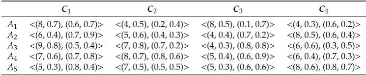
[image:18.595.110.483.296.373.2]

are all benefit-oriented indicators. The corresponding weight is w = {_{0.3, 0.2, 0.2, 0.3}}T_{, and the} decision information matrix as shown in Table1is constructed according to the decision information. In addition, considering the problem of q-RONF information aggregation based on OWA operator, the corresponding position weight vector is given asω={_{0.2, 0.3, 0.3, 0.2}}T_.

Table 1.Initial decision matrix.

C1 C2 C3 C4

A1 <(8, 0.7), (0.6, 0.7)> <(4, 0.5), (0.2, 0.4)> <(8, 0.5), (0.1, 0.7)> <(4, 0.3), (0.6, 0.2)> A2 <(6, 0.4), (0.7, 0.9)> <(5, 0.6), (0.4, 0.3)> <(4, 0.4), (0.7, 0.2)> <(8, 0.5), (0.6, 0.4)> A3 <(9, 0.8), (0.5, 0.4)> <(7, 0.8), (0.7, 0.2)> <(4, 0.3), (0.8, 0.8)> <(6, 0.6), (0.3, 0.5)> A4 <(7, 0.6), (0.7, 0.8)> <(8, 0.7), (0.8, 0.6)> <(5, 0.4), (0.6, 0.9)> <(6, 0.4), (0.7, 0.3)> A5 <(5, 0.3), (0.8, 0.4)> <(7, 0.5), (0.5, 0.5)> <(5, 0.3), (0.6, 0.6)> <(8, 0.6), (0.8, 0.7)>

Step 1 The initial decision matrixD=ai j

5×₄is normalized and the normalized matrixD=

ai j

5×₄

is obtained. The results are shown in Table2.

Table 2.Normalized decision matrix.

C1 C2 C3 C4

A1 <(0.889,0.077), (0.6,0.7)> <(0.5,0.078), (0.2,0.4)> <(1,063),(0.1, 0.7)> <(0.5,0.038),(0.6, 0.2)> A2 <(0.667,0.033), (0.7,0.9)> <(0.625,0.09),(0.4,0.3)> <(0.5,0.08), (0.7, 0.2)> <(1, 0.052),(0.6,0.4)> A3 <(1,0.089),(0.5,0.4)> <(0.875,0.114),(0.7,0.2> <(0.5,0.045),(0.8, 0.8)> <(0.75,0.1),(0.3, 0.5)> A4 <(0.778,0.064), (0.7,0.8)> <(1,0.077),(0.8,0.6)> <(0.625,0.064),(0.6,0.9)> <(0.75,0.044), (0.7, 0.3)> A5 <(0.556,0.023), (0.8,0.4)> <(0.875,0.045),(0.5,0.5> <(0.625,0.036),(0.6,0.6)> <(1,0.075),(0.8, 0.7)>

Step 2 q-RONFWA operator is used to aggregate the information in Table2to get the comprehensive q-RONFs of each scheme.

a1=<(0.717, 0.062), (0.516, 0.43)>;a2=<(0.725, 0.06), (0.635, 0.419)>; a3=<(0.8, 0.089), (0.622, 0.428)>;a4=<(0.783, 0.061), (0.71, 0.576)>; a5=<(0.767, 0.045), (0.735, 0.537)>

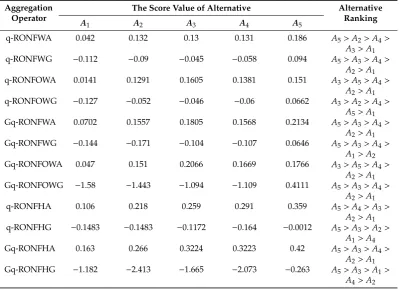
Step 3 The sorting result of score values based on q-RONFWA operator is calculated, as shown in the following:

S(A1) =0.042;S(A2) =0.132;S(A3) =0.13;S(A4) =0.131;S(A5) =0.186

Step 4 According to the score value of each scheme, 5 schemes can be ranked asA5>A2>A4> A3>A1, so the best one isA5.

6.2. Comparative Analysis

In order to analyze the validity and rationality of the proposed method in this paper, the sorting results based on different operators were analyzed, and compared with some existing methods.

[image:18.595.85.508.444.517.2]