Reshaping Elastomers with Light: First Principles Model of Diffusion-Induced Deformation

Reshaping Elastomers with Light: First Principles Model of

Diffusion–Induced Deformation

Thesis by

Ryan M. Turner

In Partial Fulfillment of the Requirements for the Degree of

Doctor of Philosophy

California Institute of Technology Pasadena, California

2012

c

2012

Acknowledgements

I would like to begin by thanking the person most directly involved in this project: my advisor, Julie Kornfield. She has been invaluable as both a source of scientific insight and knowledge as well as a personal life coach. One of the most valuable things I learned while working for her is that my career is only one aspect of my life. I am particularly thankful for the freedom to explore job opportunities, including teaching at local community colleges, while under her tutelage.

I would also like to thank my professional colleagues, particularly Anna Pandolfi for introducing me to finite elements and for fascinating conversations about science, Alan Wineman for introducing us to the ideas of mixture theory, Robin Selinger and Charles Gartland for their help in developing a point–by–point finite element implementation coupling diffusion and deformation, and Rosanna Zia for providing me with assistance in solid mechanics. I would also like to thank my other committee members, John Brady and Zhen–Gang Wang, for providing insight into theoretical questions when Julie and I were at a complete loss.

The next two people have been extremely influential in helping me finish my degree: Anne Hormann and Marcy Fowler. Thank you for ensuring that I had meeting times with Julie regardless of deadlines and for all the hard work you put into the administrative details that I’m sure we don’t always see. I also really appreciated all the advice and assistance that each of you provided in areas outside of the lab, particularly to Marcy for her support over the last couple months with all the thesis craziness. Without you two, no science would ever get done. Along that vein, I would also like to thank Kathy Bubash, Laura Lutz King, and Karen Baumgartner. In particular, Kathy’s helpfulness is one of the main reasons I decided to come to Caltech.

our Friday lunch games, and Zuli for her unending empathy, encouragement, and optimism over the past seven years.

Of course with only half of my life spent in the lab, I have a great many other people to thank. I’d like to thank my family: my mom and step–dad for supporting me through high school and undergrad, both financially and with unconditional love and emotional support; my brother Andy for helping me revise this thesis and for his friendship that has grown the last seven years; my grandma and grandpa, whom I got to know better while living with them for four months; my dad and step–mom, who have always supported me; my aunts Lois and Joy, whom I’ve always looked up to as teachers; my cousin Alan for great gaming during the holidays; and the rest of my family, that would take up a thesis in itself to list.

I’d also like to thank my friends during this period of my life: Dr. Anthony Pullen for great scientific and spiritual discussions and his wife Bethany Pullen for their friendship, Julie Moreland and her new husband Daniel, Matthew Bayless, Annie Paek, Novita Liman, Keya Schaeffer, Yoon Seo, Rob Nelson, HRock friends past and present (David Phongsa, Gabriel Ahn and all the other Covenant Brothers, the Adams, the Higashis, the Ahns, the Pokrifkas, the list goes on...). You have all supported me, encouraged me, challenged me, and taught me more than I could ever express or repay. During the past seven years, I have grown as a man because of all of you. Thank you for your friendship.

Abstract

Contents

Acknowledgements iv

Abstract vi

List of Figures xi

List of Tables xiii

List of Symbols xiv

1 Elastomeric Photopolymers 1

1.1 Development of Elastomeric Photopolymers: The Light–Adjustable Lens . . . 1

1.2 Existing Theories on Solvent–Driven Deformation of Polymer Gels . . . 6

1.3 Summary of Chapters . . . 8

2 Equilibrium Analysis from Thermodynamics 10 2.1 Introduction . . . 10

2.2 Thermodynamics of Network Swollen with Macromer before Reaction . . . 11

2.2.1 Thermodynamics of Stretching the Dry Network . . . 12

2.2.2 Initially Swollen Network . . . 13

2.2.3 Swelling Equilibrium . . . 16

2.3 Elastomeric Photopolymer after Reaction . . . 18

2.3.1 Two-Component Model . . . 21

2.3.2 Region of Validity of the Two-Component Approximation . . . 23

2.3.3 Three-Component Model . . . 32

2.4 Variational Form and Differential Equivalence . . . 36

2.5 Supplemental Material . . . 38

2.5.1 Equilibrium Swelling Data forMm = 500 and 3000 g/mol . . . 38

3.2 Kinematics . . . 41

3.3 Conservation Principles . . . 44

3.3.1 Conservation of Mass . . . 44

3.3.2 Conservation of Linear Momentum . . . 45

3.4 Constitutive Equations for the Light–Adjustable Lens . . . 46

3.4.1 Static and Dynamic Contributions . . . 48

3.4.2 Analysis of Constitutive Relations . . . 51

3.5 Conclusion . . . 54

4 Two-Cell Models 55 4.1 Introduction . . . 55

4.2 Equilibrium . . . 56

4.2.1 The Slip Case . . . 56

4.2.2 The Conforming Case . . . 59

4.3 Transient . . . 69

4.4 Conclusion . . . 75

5 Constant-Curvature Beam 76 5.1 Introduction . . . 76

5.2 Beam Constrained to a Solid Surface . . . 77

5.2.1 Stress and Strain Depend Strongly upon the Reaction Profile . . . 82

5.2.2 Effect of Material Parameters . . . 85

5.3 Beam Released to a Constant Curvature . . . 85

5.3.1 Curvature Depends Strongly upon Initial Chemical Potential Gradients . . . 94

5.4 Conclusion . . . 98

6 Light–Adjustable Lens 100 6.1 Introduction . . . 100

6.2 Computational Methodology . . . 104

6.2.1 Meshing . . . 104

6.2.2 Initialization . . . 104

6.2.3 Diffusion Step . . . 104

6.2.4 Deformation Step . . . 105

6.2.5 Separation of Time Scales . . . 106

6.3 Characterizing Deformation . . . 107

6.4 Lens-Power Adjustments Using Radial Diffusion . . . 111

6.4.2 Macromer Consumption Controls Adjustment Magnitude . . . 114

6.4.3 Effective Lens Power Depends on Pupil Dilation . . . 118

6.4.4 Parallels between Positive and Negative Adjustments of Lens Power . . . 119

6.5 Inclusion of UV Blocker Breaks Anterior–Posterior Symmetry . . . 120

6.5.1 Clinically Relevant Profiles: Positive and Negative Adjustment . . . 124

6.5.2 Lock–In: Challenges with UV Blocker . . . 126

6.6 Conclusion and Future Work . . . 130

A Governing Equations of Mixture Theory 132 A.1 Introduction . . . 132

A.2 Kinematics . . . 132

A.3 Conservation Principles . . . 134

A.3.1 Conservation of Mass . . . 134

A.3.2 Conservation of Linear Momentum . . . 135

A.3.3 Conservation of Energy . . . 138

A.4 Clasius–Duhem Inequality . . . 142

A.5 Supplemental Section . . . 143

B Material Parameters and Scaling Analysis 146 B.1 Materials . . . 146

B.2 Determination ofχ for Host Networks . . . 147

B.3 Experimental Parameters to Theoretical Parameters . . . 148

B.4 Determination of Diffusivity from Experimental Data . . . 148

B.5 Scaling Analyses . . . 151

B.5.1 Conservation of Linear Momentum . . . 151

B.5.2 Dynamic Macromer Stress . . . 152

C Finite Element Solution Method 153 C.1 Meshing . . . 153

C.2 Procedure for Mesh Creation in MATLAB . . . 156

C.2.1 Building the Full Lens . . . 158

C.2.2 Creating Mesh Visualization in MATLAB . . . 161

C.3 Interpolation . . . 163

C.3.1 Initialization . . . 166

C.3.2 Diffusion Step . . . 166

C.3.3 Deformation Step . . . 169

C.3.3.2 Movement of Nodal Points Under a Force . . . 174 C.4 Outputs . . . 175 C.5 Measurment of Local Curvature . . . 176

List of Figures

1.1 Elastomeric Photopolymer Design . . . 4

2.1 Kinematics of Deformation: Dry to Initially Swollen . . . 12

2.2 Maximum Thermodynamically Stable Volume Fraction of Macromer . . . 18

2.3 Kinematics of Deformation: Initially Swollen to Reacted and Deformed . . . 19

2.4 Material Modulus Increases with Reaction . . . 26

2.5 Values ofχ Before and After Cure for PDMS Macromer in PDMS Network . . . 28

2.6 Point–by–Point Comparison of Theory to Equilibrium Swelling Data . . . 29

2.7 Comparison of Predicted Equilibrium Swelling Data to Literature Scaling Exponents . 30 2.8 Generic Domain for Reaction–Diffusion–Deformation Problems . . . 36

2.9 Supplemental Point–by–Point Comparison of Theory to Equilibrium Swelling Data . . 39

3.1 Reference and Spatial Configuration for Mixture Theory . . . 42

4.1 Two Cells: “Slip” Deformation Model . . . 57

4.2 Deviations from Ideal Mixing for the “Slip” Case . . . 60

4.3 Deviations from Ideal Mixing for Extreme Parameter Sets . . . 61

4.4 Two Cells: “Conforming” Deformation Model . . . 62

4.5 Deviations from Ideal Mixing for the “Conforming” Case . . . 66

4.6 Parameter Space in Which an Ideal Mixing Approximation Holds Well . . . 68

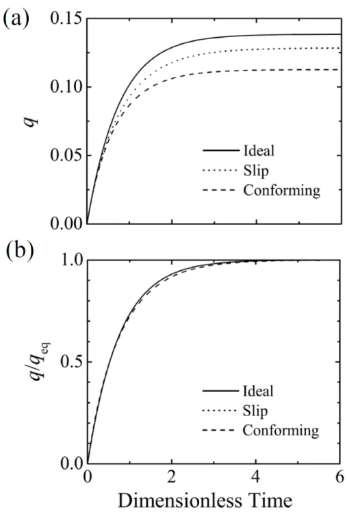
4.7 Transient Two-Cell Results . . . 73

4.8 Comparison of the Ideal Flux and Slip Flux Approximations . . . 74

5.1 Bending a Beam with Light . . . 78

5.2 Reference and Spatial Configuration for the Constrained Beam . . . 79

5.3 Constrained Stresses and Strains as a Function of Extent of Reaction Profile . . . 83

5.4 Neutral Plane Location as a Function of Extinction Length . . . 84

5.5 Constrained Stresses and Strains as a Function of Material Parameters . . . 86

5.6 Reference and Spatial Configuration for Beam Bent to Constant Curvature . . . 87

5.8 Chemical Potential after Bending . . . 95

5.9 Beam Curvature as a Function of Extent of Reaction Profile . . . 97

5.10 Beam Curvature as a Function of Material Parameters . . . 97

6.1 The Geometry of the Light–Adjustable Lens . . . 102

6.2 Change in Surface Curvature Upon Internal Irradiation . . . 108

6.3 Analogy to Multifocal Lenses . . . 109

6.4 Anterior Curvature Measured through Different Zones . . . 110

6.5 Lens Powers and Zones . . . 111

6.6 Simple Positive and Negative Adjustments . . . 112

6.7 Positive Correction from an Internal Reaction Profile . . . 113

6.8 Ripple Effect Observed at Short Times . . . 115

6.9 Effect of Material Parameters on Lens Power . . . 116

6.10 Effect of Initial Volume Fraction and Extent of Reaction on Lens Power . . . 117

6.11 Consumption of Macromer Determines Power Change Magnitude . . . 118

6.12 Power Change Across Zones . . . 119

6.13 External Consumption Causes Negative Power Changes . . . 120

6.14 Anterior and Posterior Curvature Change with UV Blocker . . . 123

6.15 Effect of Decaying Irradiation on a Simple Positive Adjustment . . . 123

6.16 Sample Clinical Extent of Reaction Profiles . . . 124

6.17 Clinical Positive Adjustment vs. Internal Top Hat Profile . . . 125

6.18 Clinical Positive and Negative Adjustments with UV Blocker . . . 126

6.19 Uniform and Clinical Lock–in with UV blocker . . . 128

6.20 Lock–In of Clinical Adjusments . . . 129

A.1 The Kinematics of Mixture Theory . . . 133

B.1 Chemical Structure of PDMS . . . 146

B.2 Chemical Structure of Macromer . . . 146

B.3 Experimentally Obtained Floryχ Interaction Parameter Values . . . 147

B.4 Diffusivity of PDMS Macromer in PDMS Network . . . 150

C.1 Cross–Section of Lens Mesh . . . 154

C.2 Light–Adjustable Lens Mesh . . . 155

C.3 Cross–Sections of the Base Subset . . . 160

C.4 Visualization of the Base Subset . . . 161

List of Tables

2.1 Scaling Exponents Obtained from the Modified Flory–Rehner Equation . . . 31

6.1 Geometric Parameters for the Light–Adjustable Lens . . . 101

6.2 Determination of Diffusion Time Scales from Lens Length Scales . . . 106

6.3 Computational Parameters Used at Short and Long Times . . . 107

6.4 Real Times for Each Regime of Diffusion–Deformation Behavior . . . 114

6.5 Even Function Coefficients for Clinical Radial Profiles . . . 124

B.1 Linear Regression Parameters forχas a Function ofG_{dry . . . .} 148

B.2 andχParameters Corresponding to Experimental Variables . . . 148

B.3 Diffusivities of PDMS Macromer in PDMS Network . . . 150

B.4 Experimentally Determined Viscosity of PDMS at Two macromer Molecular Weight . 152 C.1 Initial Mesh Volume and Surface Area . . . 156

C.2 Base Subset Nodal Locations . . . 159

List of Symbols

a (§4.2.2) Length scale . . . 59

A Dimensionless Helmholtz free energy per unit volume . . . 16

(Ch. 4) Cross–sectional area . . . 70

(§6.5.1) Even function coefficient . . . 124

α (§2.3) Modulus vs. swelling exponent . . . 29

(Ch. 5) Dimensionless neutral axis position within the beam . . . 77

αi (§2.2) Principle stretch inith direction . . . 13

b, bi Internal body force per unit volume exerted by macromer on network . . . 45

ˆ b,ˆbi (§3.4.1) Static internal body force . . . 48

e b,ebi (§3.4.1) Dynamic internal body force . . . 48

B (§6.5.1) Even function coefficient . . . 124

β (Ch. 4) Radial stretch factor . . . 59

(Ch. 5) Interior angle used to determine beam curvature . . . 88

C (§6.5.1) Even function coefficient . . . 124

χ Flory interaction parameter . . . 14

χ, χi Mapping from dry network to spatial configuration . . . 12

χ∗, χ∗_i Mapping from initially swollen network to spatial configuration . . . 38

χ_m, χm i Mapping from macromer reference to spatial configuration . . . 42

χN, χNi Mapping from network reference to spatial configuration . . . 42

di Irradiation diameter . . . 107

dse Diameter for the interior of the square–edge . . . 101

d Total lens diameter . . . 101

df Central zone diameter: pupil constricted, far-distance vision . . . 109

dn Near zone diameter: near-distance vision . . . 110

dp Peripheral zone diameter: peripheral vision . . . 110

D (§6.5.1) Even function coefficient . . . 124

D Diffusivity of macromer in network . . . 50

D

Dt Total derivative (A.5.10) . . . 145

D(m) Dt Partial total derivative with respect to macromer (3.4.5) . . . 47

D(N) Dt Partial total derivative with respect to network (3.4.8) . . . 48

δ(t) (§2.3) Delta function . . . 22

δ (§2.3) Small shear strain . . . 24

(§4.2.1) Deviation of swelling from ideal mixing . . . 58

δij,I Identity tensor . . . 24

ec, ecij (§3.4.2) Conforming strain . . . 53

Ratio of stretching energy scale to osmotic energy scale . . . 15

0 modified for the three–component model . . . 35

f (§6.5) Extent of reaction function . . . 121

∆F Helmholtz free energy relative to reference, extensive . . . 13

∆Fel Elastic stretching Helmholtz energy, extensive . . . 34

∆Fmix Helmholtz free energy of mixing, extensive . . . 14

F Dimensionless system free energy . . . .36

e F (Ch. 2) Dimensionless system free energy including constraint . . . 37

F, FiJ Deformation gradient relative to dry network . . . 12

F∗_{, F}∗ iJ Deformation gradient relative to initially swollen network . . . 19

F_iJextract Deformation gradient associated with extraction . . . 24

FN, FiJN (§3.2) Network deformation gradient, mixture theory . . . 43

Fc, FiJc (§3.4.2) Conforming deformation gradient . . . 52

φ, φm Volume fraction of macromer . . . 43

¯ φ Average volume fraction in a system after reaction . . . 81

φ0 Volume fraction of macromer in the initially swollen gel . . . 18

φ1 (Ch. 4) Macromer volume fraction in cell 1 . . . .56

φ2 (Ch. 4) Macromer volume fraction in cell 2 . . . .56

φ0eq Equilibrium volume fraction of macromer after reaction . . . 27

φf Volume fraction of fixed species . . . 32

φi (§6.5.2) Equilibrium volume fraction of macromer afterith reaction . . . 127

φ_max Maximum allowable initial volume fraction of macromer . . . 17

φm,eq Equilibrium volume fraction of macromer after reaction . . . 17

φn Volume fraction of nodules . . . 33

φN Volume fraction of network . . . 43

ϕ Cylindrical azimuthal coordinate, spatial configuration . . . 88

Φ Cylindrical azimuthal coordinate, reference configuration . . . 102

g (§6.5) Extent of reaction function . . . 121

G Dimensionless shear modulus after curing, drying, and reswelling . . . 32

¯ G Average of spatially varying modulus . . . 82

Gc Dry composite modulus of network with filler . . . 34

G_cured The dry network modulus after cure . . . 25

G_dry Modulus of initial, dry network . . . 14

Gos Osmotic modulus . . . 15

G_shear Shear modulus after curing, drying, and reswelling . . . 31

∆G Gibbs free energy, extensive . . . 14

γ (§3.4.1) Macromer constitutive law parameter (bulk viscosity) . . . 50

hmax Thickness of the lens at the center . . . 101

hmesh Mesh size (smallest distance between two mesh points) . . . 106

hmin Thickness of the lens haptics . . . 101

H Length scale . . . 69

H Curvature . . . 89

∆Hmix Enthalpy of mixing, extensive . . . 14

I Light intensity profile . . . 21

I, δij Identity tensor . . . 16

Jc (Ch. 4) Flux of macromer for the “conforming” case . . . 71

J_id (Ch. 4) Ideal mixing flux of macromer . . . 71

Js (Ch. 4) Flux of macromer for the “slip” case . . . 69

Jm, Jm i Flux of macromer . . . 44

JN, JN i Flux of network . . . 44

k Boltzmann’s constant . . . 13

κ (Ch. 4) Deviation of “conforming” case from “slip” case . . . 72

l (Ch. 5) Length of hypothetical line at the neutral plane . . . 88

λ (§2.3.3) Kerner parameter for three–component model modulus . . . 34

(Ch. 5 and Ch. 6) Extinction length . . . 77

λα (Ch. 4) Axial stretch in cellα . . . 59

Λα (Ch. 4) Ratio of axial to radial stretch in cellα . . . 63

mN0 (§2.2)Dry network mass . . . 14

Mc Molar mass between crosslinks for the original network . . . 11

Mm Macromer molar mass . . . .15

Mp Precursor network chain molar mass . . . 11

µm Chemical potential of macromer in a gel . . . 16

µ Dimensionless chemical potential of macromer relative to pure . . . 17

(§3.4.1) Macromer constitutive law parameter (viscosity) . . . 50

µα (Ch. 4) Isotropic chemical potential in cellα . . . 58

µconf α (Ch. 4) Effective chemical potential in cellαfor the conforming case . . . 63

µcons (Ch. 5) Effective chemical potential for the constrained beam . . . 81

µbent (Ch. 5) Effective chemical potential for the beam bent to curvatureH . . . 94

nA (Ch. 6) Refractive index of the aqueous humor . . . 107

nα (Ch. 2) Number of molecules of speciesα . . . 14

nL (Ch. 6) Refractive index of the lens . . . 107

n, ni Surface normal . . . 37

Na Avogadro’s number . . . 15

νe Number of elastically effective strands . . . 13

νN Network Poisson ratio . . . 34

p Lagrange multiplier at equilibrium . . . 37

P (Ch. 6) Lens power . . . 110

P0 (Ch. 6) Initial lens power . . . 110

∆P (Ch. 6) Change in lens power . . . 110

P, PiJ First Piola–Kirchhoff stress tensor . . . 37

Π Osmotic pressure . . . 17

q (Ch. 4) Fractional volume change . . . 58

(Ch. 5) Deformation field associated with the constant curvature beam . . . 89

qc (Ch. 4) Fractional change in volume, “conforming” case . . . 72

q_id (Ch. 4) Fractional change in volume for the ideal mixing approximation . . . 58

qs (Ch. 4) Fractional change in volume, “slip” case . . . 72

Q Volume ratio relative to the dry network . . . 22

Q∗ Volume ratio relative to the initially swollen network . . . 23

Q∗_reswell (§2.3.2) Volume ratio after curing, drying, and reswelling . . . 31

Q0 Initial swelling ratio . . . 19

Qeq Equilibrium swelling ratio of unreacted system . . . 17

Q0_eq Equilibrium swelling ratio after reaction . . . 27

Qi (§6.5.2) Equilibrium volume fraction after reactioni . . . 128

QR Volume ratio of volume before reaction to that after reaction . . . 32

θ Conversion parameter; volume of current network to dry network . . . 22

θ∗ Conversion parameter relative to initially swollen network . . . 23

θi (§6.5.2) Conversion parameter for theith reaction . . . 128

Θ (§3.4) Term arising in the Clausius–Duhem equality (A.4.8) . . . 47

r Cylindrical radial coordinate, spatial configuration . . . 106

rm Rate of creation of macromer per unit spatial volume . . . 22

rN Rate of creation of network per unit spatial volume . . . 44

R (Ch. 2) Universal gas constant . . . 14

(Ch. 5) Radius of curvature of beam . . . 89

(Ch. 6) Cylindrical radial coordinate, reference configuration . . . 102

Ra Anterior lens radius . . . 101

Rp Posterior lens radius . . . 101

ρ Spatial density field . . . 43

ρm Macromer density field, spatial configuration . . . 43

ρm0 Density of pure macromer . . . 15

ρn0 Pure density of nodules . . . 32

ρN Network density field, spatial configuration . . . 43

ρN0 Density of pure network . . . 14

∆S Entropy relative to reference, extensive . . . 13

∆Smix Entropy of mixing, extensive . . . 14

dS Differential surface area . . . 37

σ, σij Cauchy stress tensor . . . 38

σm, σijm Partial Cauchy stress of macromer . . . 45

σN, σijN Partial Cauchy stress of network . . . 45

ˆ σα,σˆα ij (§3.4.1) Static partial Cauchy stress of speciesα . . . .48

e σα,_eσα ij (§3.4.1) Dynamic partial Cauchy stress of speciesα . . . 48

σc, σc ij (§3.4.2) Anisotropic stress contribution . . . 53

t Time . . . 19

td (§6.2.5) Time scale associated with gradients in ther–direction (d/2) . . . 106

th (§6.2.5) Time scale associated with gradients in thez–direction (hmax) . . . 106

∆T (§6.2.5) Dimensionless time step . . . 106

T Dimensionless time . . . .70

T (Ch. 2) Absolute temperature . . . 13

τ (§2.3) Shear stress . . . 24

(Ch. 5) In-plane stress . . . 81

(§C.3.2) Time scale . . . 167

τα (§4.2.2) Tensile stresses in cell α . . . 64

τϕ (Ch. 5) Relative stress difference in the bent beam . . . 90

vm, vim Spatial velocity field of macromer . . . 43

vN, vN i Spatial velocity field of network . . . 43

v, vi Barycentric velocity field . . . 43

V Spatial volume . . . 13

V0 Initial volume . . . 37

Vα (Ch. 4) Volume of cellα . . . 70

Vm Spatial volume of macromer . . . 15

Veq Volume at equilibrium . . . 37

VN Spatial volume of network (initial, plus that inherited by reaction) . . . 15

dV Differential volume, spatial configuration . . . 12

dVd _{Differential volume, dry network . . . 12}

dV0 Differential volume, initially-swollen network . . . 19

dVα Differential volume of speciesα . . . 32

dVα0 Differential volume of speciesαin reference . . . 32

dVf Differential volume of fixed species . . . 32

dVR Differential volume right after reaction . . . 32

W External work, extensive . . . 14

Ωd _{The dry network body; reference configuration (§2.2) . . . 11}

Ω0 Initially swollen network body; reference configuration (§2.3 onward) . . . 11

Ω(t) Spatial configuration body . . . 19

∂Ω1 Boundary of Ω(t) on which deformation is specified . . . 36

∂Ω2 Boundary of Ω(t) on which stresses are specified . . . .36

Ωm Reference configuration for macromer, mixture theory model . . . 42

ΩN Reference configuration for network, mixture theory model . . . 42

x Cartesian coordinate, spatial configuration . . . 88

x, xi Spatial position . . . 19

X Cartesian coordinate, reference configuration . . . 76

Xd, Xd I Reference position (§2.2) . . . 11

X Reference position,XI (§2.3 onwards); spatial position,Xi (§2.2) . . . 11

Xm, XIm Reference position for macromer, mixture theory model . . . 42

XN, XIN Reference position for network, mixture theory model . . . 42

ξ Extent of reaction . . . 22

ξi (§6.5.2) Extent of reaction profile for the ith reaction . . . 128

ξI (Ch. 5 and 6) Surface extent of reaction nearest the light source . . . 77

y Cartesian coordinate, spatial configuration . . . 88

ψ Transient Lagrange multiplier, mixture theory . . . 47 ˆ

ψ Static portion of the Lagrange multiplier, mixture theory . . . 51 e

ψ Dynamic portion of the Lagrange multiplier, mixture theory . . . 51

z Cartesian coordinate, spatial configuration . . . 88

Chapter 1

Elastomeric Photopolymers

1.1

Development of Elastomeric Photopolymers: The Light–

Adjustable Lens

A cataract is a clouding of the intraocular lens in the eye due to changes in protein structure [2]. Cataracts are very common: over 1.5 million cataract surgeries are performed yearly in the United States alone and over 60% of people over the age of 60 have cataracts [2]. In tandem with the population progressively living to older age, cataract surgery has developed from the primative method of couching—a procedure in which the cloudy lens was dislocated into the vitreous cavaity of the eye by being struck with a blunt object—to modern surgical methods [3]. Current surgical methods make use of a two-step procedure. First, the cloudy lens is removed via phacoemulsification, a procedure in which the cloudy lens is shattered with ultrasound and the pieces removed through a small incision. Using the same incision, a foldable intraocular lens is surgically implanted to replace the old lens.

adjustable after operation.

Because of the position of the lens in the eye post–operation, a reasonable non–invasive adjust-ment would involve light. For example, an entire branch of research has centered around light-activated polymers [7]. One class of materials developed are liquid crystal elastomers (LCE) which can undergo deformation due to isomerization in the presence of light. Theory has been developed to predict that LCE beams will curve when exposed to Beer’s law decaying light profiles through the depth [8–12]; bending an initially flat beam creates an optical element. Because such shape changes are non–invasive and reversible, these materials show particular promise for applications in microfluidics [13]: examples include light–driven micropumps [14], micro cantilevers [15], and opti-cally driven nanoscale actuators [16]. However, because the shape changes in LCEs are reversible and imprecise and the materials themselves tend to be relatively opaque, these materials would not produce a reasonable intraocular implant. A more translucent material is necessary and the shape changes need to be stable and reproducable with a fine degree of precision.

A second type of material that meets these qualifications is a photopolymer [17]. A photopolymer consists of a glassy polymer backbone filled with small monomor particles. Irradiation with light causes monomer particles trapped inside the polymer backbone to photopolymerize, causing local volume changes as well as local changes in refractive index and modulus. Because the photopoly-merization is permanent and a large degree of control can be exerted on the light–source, submicron features which are permanent and precise can be written into a photopolymer and stored; for this reason, a main application of photopolymers is in holographic storage devices [18, 19]. However, these materials have several limitations. First, the polymers used are glassy, inhibiting their use in intraocular lenses that must be folded and inserted through a small incision during surgery. More importantly, the glassy nature of the polymer makes diffusion occur exceedingly slowly and write times are only reasonable for changes on the order of microns. Although this is appropriate for holo-graphic storage, the write time would be prohibitively long for adjustments to an object of the length scale of millimeters, such as an intraocular lens. Lastly, the materials used for these photopolymers are toxic: monomer can leach out of the polymer backbone and into the eye.

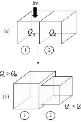
original host network (Fig. 1.1c). The depletion of free macromer by the polymerization reaction creates chemical potential gradients in the polymer gel: the chemical potential is higher in zones that were not irradiated since they have more macromer. These gradients drive diffusion of the free chains from the non–irradiated regions into the irradiated regions. Since the elastomeric photopolymer is an incompressible gel, the transfer of mass between regions results in local volume changes as the macromer chains diffuse. The regions that were irradiated swell as there is a net influx of mass, whereas the regions that were not irradiated shrink as they lose mass to the irradiated regions. This causes a net global shape change (Fig. 1.1d). To maintain the desired shape of the photopolymer for long–term use, the material can be uniformly irradiated to cross–link any left-over free molecules once the desired shape has been obtained (Fig. 1.1e). This “locks in” the shape of the material and prevents possible leaching of the free chains or photoinitiator into the surrounding medium. A lens crafted of elastomeric photopolymer can then be non–invasively adjusted after operation by selective irradiation [20].

Clinically, the light–adjustable lens is implanted in the patient and wound healing is allowed to occur. Once the lens has stabilized, a clinician can use a Fitzeau interferometer to determine the precise correction needed by that patient to achieve emmetropia [21]. Clinically, the irradia-tive “adjustment” proceeds for a minute or two and the material is designed so that the resulting diffusion–deformation process is complete within 12–18 hours [4]. The clinician then examines the patient and determines whether subsequent corrections are necessary; because only small amounts of macromer need to be consumed to achieve necessary corrections [4], plenty of free macromer remains available for subsequent correction. Once all corrections have been made, the final shape of the lens is “locked in” by reacting the remaining macromer using a stronger irradiation than that used during the treatment. This guarantees that any created change in lens shape will be stable and eliminates the possibility of reactive molecules transferring from the lens to the body in future years.

to examine the underlying physics which would provide a tool–kit for nomogram design, the clinic continues to operate through experimental trial and error.

In earlier work, Pandolfi and Ortiz made a first attempt to explain the underlying physics of the light–adjustable lens [27]. Although the model developed therein successfully predicted final lens power changes, the simulations developed were unable to predict the kinetics of shape change. To clinicians, the rate at which the adjustment occurs is of as much importance as the magnitude of the adjustment itself. In addition, the model made no connection to material design parameters, despite the availability of experimental data [1] and the nomograms presented are parameter fit from nomograms already established through experimental trial and error. In this sense, the model developed is more reactive than predictive. Given the limitations of this preliminary theoretical work, we set out to propose a model based upon first principles which could be used to predict both the rate and the magnitude of shape changes experienced in elastomeric photopolymer lenses.

One of the primary goals of this work is to connect theory with experiment. The data presented in Pape’s Ph.D. thesis [1] provides a starting ground for modeling from first principles. This work considers all the material design parameters necessary in creating an elastomeric photopolymer: initial network creation, extent of equilibrium swelling with macromer as well as rates of diffusion, and reaction rates for the photopolymerization process. Because the materials used therein consist of a PDMS network with PDMS bis–methacrylate end–capped macromers (§B.1), we also draw upon experiments and theory performed by Cohen and co–workers [28–31]. In this manner, we seek to develop a theoretical tool–kit founded on experimentally adjustable material parameters which predicts the effects of those parameters on the magnitude and rate of shape change.

1.2

Existing Theories on Solvent–Driven Deformation of

Poly-mer Gels

We begin by discussing existing theoretical work on diffusion–deformation behavior in polymer gels. The pioneering work on the swelling of polymer gels is attributed to Flory and Rehner [32–35]. Using statistical mechanics, the network chains are modeled as random walks. Under the action of a solvent, the network chains stretch and they experience a net decrease in entropic configurations. The solvent, on the other hand, experiences a net entropic gain by mixing with the network. Equilibrium is established when these two entropic forces are in balance: the amount of macromer that can swell into a given gel is determined by thermodynamics. The choice of material parameters, then, sets limits on the amount of initial material available for reaction–diffusion in elastomeric photopolymers. We extend the work of Flory and Rehner in Ch. 2 to elastomeric photopolymers.

The first proposed model of the kinetics of diffusion in polymeric gels is due to Tanaka, Hocker, and Benedek [36], later modified by Tanaka and Fillmore [37]. The original model was successful at predicting the kinetics of swelling spherical gels but failed for general anisotropic swelling [38]. Only recently has a body of work been developed which can successfully capture general anisotropic swelling behavior: the stress–diffusion coupling model (SDCM) [39–41]. This theory couples polymer diffusion to deformation by using an equivalent of Darcy’s law, treating the gel as a porous solid. Although the authors have successfully applied this model to several anisotropic problems [40–44], their work is based on external pressure gradients driving flow into the gel. As such, they are able to treat the volume fraction inside the gel as constant in time, implying that the gel is always in chemical equilibrium with the solvent bath. In our applications, the material is self contained: there are no external pressures driving flow into the gel. Furthermore, it is the spatially varying nature of the volume fraction field coupled to local concentration of volume that causes shape change. For this reason, the use of the SDCM equivalent of Darcy’s law would be inappropriate for elastomeric photopolymers.

performed in [52] solely because the developed constitutive relations do not take the second law into account. Because mixture theory allows the direct incorporation of thermodynamic knowledge into the constitutive equations, we can systematically develop constitutive laws predicting the stress and kinetics in elastomeric photopolymers from first principles.

Since its inception in the 1960s, mixture theory has provided a rigorous framework for treating previously intractable problems in a variety of fields. Early successes in mixture theory included modeling the flow of a Newtonian fluid through an elastic solid [53], propagation of waves through a solid–liquid mixture [54], and deformation of a mixture of two non–linear elastic solids [54]. More recently, applications have blossomed to include modeling of phase transitions and particulate mix-tures (see [55] for sources and more examples). Mixture theory has also been used to model growth processes in biology for use in fields such as cartilage engineering [51, 56, 57], muscle and tendon engineering [52], and in modeling the aorta [58].

Rajagopal, Wineman and coworkers have used mixture theory to model the transient swelling of a polymer network due to solvent [59]. Using a free energy for swelling given from general polymer physics [60], the authors derive constitutive relations for the partial stress tensors of both the solvent and the polymer that implicitly satisfy the second law of thermodynamics. After neglecting inertial effects and body forces, the authors solve a steady, one–dimensional problem in which a fluid is moving through a polymeric solid in a variety of geometries [59, 61–63]. Although the only experimental data with which the authors could compare results was in the case of pressure-driven flow through a flat plate [64], the non–linear diffusive behavior observed in experiment was successfully predicted [59].

Around the same time, simultaneous approaches not requiring a dissipative functional were developed by a number of authors [72–76]. Like mixture theory, these authors make use of the second law of thermodynamics to postulate a constitutive law for the flux of solvent into a swelling gel. The differences between each of these models is minor and all authors solve one or two types of problems: force and deformation of a gel caused by an externally imposed flux of macromer, or the flux of macromer caused by an externally imposed mechanical force. None of these developed theories provide a framework for a force-free, self–contained elastomeric photopolymer in which deformation is caused by reaction due to a light source.

This thesis expands the works of the above authors by including the effects of reaction spe-cific to elastomeric photopolymers. In the photopolymer, many components are present and have particularly complex time dependence during and shortly after irradiation: photoinitiator, radical fragments of the photoinitiator, propagating radicals, unreacted macromer, original host network, and interpenetrating network (IPN) formed by polymerization of macromer. In addition, passive dye molecules may be included to attenuate light with depth in the sample. As a preliminary model, we make several simplifying approximations. Based on clinical experiments in which the photopolymer is only exposed for a short amount of time (<5 min) relative to the time it takes for diffusion (≈1 day), we first treat reaction as instantaneous. In addition, we furthermore treat the initial extent of reaction as a one–to–one mapping with the irradiation field, rather than specifying the complexities of ray tracing and other optical effects. Finally, experimental characterization of photoelastomers has revealed that the effective crosslink density of the network is only weakly modified by forma-tion of the IPN: the elastic modulus increases by less than a factor of two [1]. We will show that, to good approximation, this allows the created IPN to be modeled as additional network strands supplementing the original network; that is, a specified extent of reaction profile will be assumed to convert macromer directly into network. Although it is not a priori obvious that this “two-component model” is a good approximation, we will show that the model can successfully capture the qualitative behavior of elastomeric photopolymers.

1.3

Summary of Chapters

The remainder of this thesis proceeds as follows:

good approximation is discussed and a small adjustment to this model (the “three-component” model) is proposed for regions in which the two-component model fails. Finally, a methodology is proposed in which the equilibrium shape of an elastomeric photopolymer can be found from the initial extent of reaction profile by minimization of the free energy functional developed.

• Chapter 3 presents the framework for solution of general transient problems in terms of mixture theory. The governing differential equations are shown to be the same as those obtained from the variational approach derived in Ch. 2. In addition, the second law of thermodynamics is used to postulate a constitutive relationship between the flux of macromer and a driving force. The resulting kinetic law is examined and compared to the work of other authors.

• Chapter 4 takes the theory developed in Ch. 2 and 3 and applies it to a simple case of two small elements in thermodynamic contact. To illustrate the importance of the various material parameters, two systems are studied: one in which chain stretching is completely ignored (the “slip” case) and the other in which chain stretching is included (the “conforming” case). These studies examine simplifications that can be made to the model based upon the appropriate clinical parameter space.

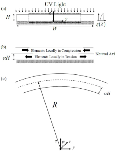
• Chapter 5 applies the theory of Ch. 2 to a beam constrained to a solid surface. This expands the two-cell model to a system with one–dimensional gradients due to the extent of reaction profile. The stresses and strains generated are predicted and connected to material parameters and reaction profile parameters. In addition, the developed stresses and strains are used to determine the deformation the beam would attain were it released and allowed to attain a constant curvature.

Chapter 2

Equilibrium Analysis from

Thermodynamics

2.1

Introduction

We begin our study on predicting the reaction–induced deformation of elastomeric photopolymers by first considering their thermodynamics. It is the balance between stretching of network chains and mixing free energies which gives our materials, their unique properties. We must therefore develop a free-energy based upon this balance; minimization of this free energy will drive the deformation of the material in time. The free energy developed must be consistent with first principles and have a connection to experimentally determined material parameters. It must be able to correctly predict the swelling and mechanical properties of these materials as well as provide a connection between reaction–diffusion–deformation. The conclusion to this chapter presents an energy minimization method which determines the final equilibrium shape for a system; we will show in Ch. 3 how the same free energy can also be used to solve transient problems with mixture theory.

sufficient to predict both the increase in material modulus experienced upon photocuring and the equilibrium swelling behavior of photocured samples. The three-component model is shown to be a plausible correction to the two-component model in the case where the nodular nature of the macromer upon reaction becomes more important. We finish this chapter by illustrating the energy minimization principle that will be used throughout the rest of this work. This energy minimization is shown to lead to the same relations as those obtained through classical continuum mechanics (discussed in Ch. 3).

2.2

Thermodynamics of Network Swollen with Macromer

before Reaction

Consider a host of precursor chains having an average molar massMp and some known polydisper-sity index. We first consider the pure host network formed from these precursor chains, through some cross–linking process. The character of the network is measured in terms ofMc, the average molecular weight of a network strand between cross–link junctions. In general, this value will be different from Mp because of the possibility of loops, dangling chains and other structural defects depending upon reaction conditions and the functionality of the cross–linker [28]. In addition, there is also discussion in the field as to whether entanglements act as crosslinks or restrict the motion of crosslinks [30]. For the purposes of our discussion here, we will take the character of the network to be defined by the shear modulus after the sample has been cured and any solvent has been ex-tracted (denoted G_{dry). In practice, the value of} Mc is deduced from the modulus and represents an estimate on the length between network strands, hiding the details of network defects (dangling chains, loops, entanglements, etc.). Theoretical results will be compared to the results of Pape who carefully chose reaction conditions to minimize the number of defects inherent in the network [1].

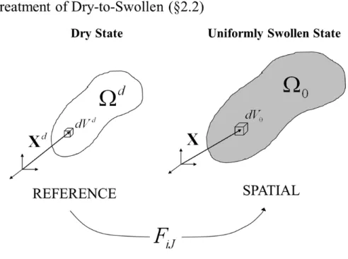
We now examine deformations of this host network; this will be useful in modeling how chains are stretched upon swelling with solvent. Since the crosslinked network has not yet been swollen, we call this material the “dry network.” To denote variables related to this stage, we use d as a superscript. For example, we label the region of space that the crosslinked network occupies as Ωd (Fig. 2.1). We take this initial, dry network as the reference configuration for this section (§2.2). The position of each material point in Ωd is marked by a vector Xd relative to some coordinate system. When the dry network is put in a bath of solvent, it swells. Let the swollen configuration of the object be Ω0; this is the spatial configuration for this section (§2.2, note that it becomes the reference configuration in §2.3). Each spatial point is given a different label X . We use Einstein and Berkeley notation throughout: the subscript that indicates the vector component is upper case for the reference configuration (Xd

I being equivalent toX

Figure 2.1: The kinematics of deformation in §2.2: A dry host network (occupying Ωd_{) absorbs} small-molecule macromer chains to occupy the region Ω0. Note that the superscript “d” is used throughout this thesis to indicate the “dry state” and is not an exponent.

configuration and each spatial point

Xi=χi(Xd). (2.2.1)

The gradient of this mapping

FiJ(Xd) =

∂χi(Xd)

∂Xd J

, (2.2.2)

is the deformation gradient. For example, the determinant ofFiJ measures local volume changes

detFiJ =

dV

dVd. (2.2.3)

HeredVdis the infinitesmal volume of the material point located atX_Idin the reference configuration anddV is the volume of that point after it is swollen and located atXi.

2.2.1

Thermodynamics of Stretching the Dry Network

the material along three directions in an orthonomal basis is [35]:

∆S=−kνe

2

αx2+α2y+αz2−3−ln (αxαyαz)

. (2.2.4)

Here,kis the Boltzmann constant,νeis the number of effective elastic chains andαiis the principle stretch in theith orthonormal direction. To be more general, we rewrite this expression in terms of a lab reference frame using the deformation gradientFiJ:

∆S=−kνe

2

trFiJFjJ−3−ln detFiJ

. (2.2.5)

Note that only the invariants ofFiJcan contribute to the free energy since the system energy has to be independent of any solid body rotation of the sample. The first term, trFiJFjJ−3, represents the decrease in configurational entropy of the Gaussian chains as caused by the externally imposed deformation. It will be positive in swelling deformations, since swelling will stretch the network chains and decrease the entropy of the system. The second term, ln detFiJ, does not appear in most works on polymeric elastomer deformation because, to good approximation, it is incompressible (detFiJ = 1). In the case of a swelling deformation, however, the final volume through which the chains are distributed increases. This increased volume yields more available configurations to the network cross–links and therefore acts to increase the entropy of the system, in sharp contrast to linear chain stretching effects [77].

2.2.2

Initially Swollen Network

When a dry network is placed in contact with a reservoir of small chain macromer molecules, entropic contributions drive the diffusion of the chains into the network, causing it to swell. There are now three contributions to the system energy: 1) the energy of stretching the host network chains as macromer is imbibed; 2) the entropy gained through the mixing of host network and macromer chains, and 3) the enthalpy cost due to solvent–solute interactions. We now introduce the subscripts

m to refer to the free macromer species and N to refer to the network. Here, we are concerned with deformations induced by the osmotic pressure of the bulk solvent. The corresponding stress (illustrated below,O(106Pa)) is much less than the stress required to fully extend network strands. Therefore, the bond lengths and angles are not perturbed and, consequently, the internal energy is unchanged (∆U = 0). The change in system free energy is then purely entropic (∆F =−T∆S). Per unit of spatial volume,V, the change in elastic stretching free energy due to swelling is

∆F V =−T

∆S V =

1

2GdryφN

trFiJFjJ−3−ln detFiJ

Note that the prefactor in (2.2.6) has been rewritten in terms of G_{dry, the original, dry network}

shear modulus:

G_{dry =} kT νe Vd =

mN0RT

McVd

= ρN0RT

Mc

, (2.2.7)

where mN0 is the mass of the network, ρN0 is the pure network density, and R is the universal gas constant; the factor of φN = Vd/V, the volume fraction of network, takes into account that only network chains are stretched in a swollen gel. Because the system is swelling, the local volume changes

detFiJ =

dV dVd =

1

φN

(2.2.8)

are non–zero: φN ≤1 so detFiJ≥1 as the material swells.

Aside from an energetic penalty due to solvent–solute interactions, we assume ideal mixing of our two components. If the pure component densities of macromer and network are the same, there will be no change in volume upon mixing; experimental measurements confirm this to good approximation [1]. Following [35], the mixing entropy gain for bringing two pure-component polymer species together is

∆Smix=−k(nmlnφm+nNlnφN), (2.2.9) where nα is the number of molecules of species αand φα is the volume fraction of species α. As noted by Flory, nN = 1 nm for a system in which component N is a single molecule (i.e, a cross–linked network). Therefore, the network contribution to mixing entropy is negligible. This gives an effective entropy of mixing of

∆Smix=−knmlnφm. (2.2.10)

Although it is generally less than the entropy of mixing, there can also be an enthalpy change upon mixing chemically dissimlar components. The simplest approximation for this is a linear variation with the number ofN–mcontacts:

∆Hmix=kT χnmφN, (2.2.11)

whereχis a binary interaction parameter measuring the energy penalty per repeat unit of macromer. Whenχis positive, the network–macromer contact is unfavorable and mixing is penalized. The free-energy change of mixing macromer into a dry network is a combination of (2.2.10) and (2.2.11):1

∆Fmix=kT nm(lnφm+χφN). (2.2.12)

1_{This is only true in the absence of external work. In general, ∆G= ∆H−T∆S= ∆F+W whereW is the work}

In stating these relations, we have made the same assumptions as Flory, including ignoring volume change on mixing and packing effects due to differences in macromer and network volume. Depar-tures from these assumptions can be corrected by making the χ parameter dependent upon other parameters (such as temperature) but we do not do so here.

Noting thatnmis related to the pure component density of macromerρm0by

nm=

ρm0Vm

Mm

NA (2.2.13)

(Vmbeing the volume of macromer,Mm the macromer molar mass, andNA Avogadro’s number ), and with the definition of macromer volume fractionφm=Vm/V, (2.2.12) can be written as

∆Fmix

V = ρm0RT

Mm

φm

lnφm+χφN

. (2.2.14)

We define the prefactor for the mixing term asGos, the osmotic modulus:

G_{os =} ρm0RT Mm

. (2.2.15)

Since we assume no volume change upon mixing,V =Vm+VN andφm+φN = 1 (see [78]) so that the free energy of mixing depends only uponφm.

Combining the contributions of mixing (2.2.14) and stretching (2.2.6), the total free energy per unit volume is

∆F

V =Gdry

1 2φN

trFiJFjJ−3−ln detFiJ

+Gosφm

lnφm+χφN

. (2.2.16)

From this expression, we see that there are two characteristic energy scales: one energy density is the osmotic modulus Gos generated by the mixing of macromer and the other the shear modulus

G_{dry due to the stresses borne by the network. As has been seen, both are entropic in origin. For}

the case in which the pure component density of macromer and network are the same (ρm0=ρN0), the two are not independent: their ratio depends upon the single parameter:

≡ Gdry

Gos =

Mm

Mc

. (2.2.17)

scale with which we define thedimensionless free energy per unit volume,A:

A(FiJ, φm, φN)≡ ∆F

GosV =φmlnφm+χφmφN +

1 2φN

trFiJFjJ−3−ln detFiJ

. (2.2.18)

The first term represents ideal mixing, whereas the other two terms can be considered corrections due to (1) enthalpy of mixing effects (which scale withχ) and (2) chain stretching (which scale with

). The smaller the size of macromer chains relative to network chains, the less chain stretching affects the system energy.

2.2.3

Swelling Equilibrium

When a dry network sample is placed in a bath of macromer, it swells until it reaches a point at which the decrease in free energy due to the entropy of mixing macromer into the network becomes equal to the free energy cost of elastic stretching of network strands. This state of swelling equilibrium is closely related to osmotic equilibrium, as aptly stated by Flory:

“A close analogy exists between swelling equilibrium and osmotic equilibrium. The elastic reaction of the network structure may be interpreted as a pressure acting on the solution, or swollen gel. In the equilibrium state this pressure is sufficient to increase the chemical potential of the solvent in the solution so that it equals that of the excess solvent surrounding the swollen gel. Thus the network structure performs the multiple role of solute, osmotic membrane, and pressure generating device.” [35]

In this section, we review swelling equilibrium to convey the physical significance of our expression for the free energy [35]. For a system swollen with macromer, the difference between the chemical potential of macromer inside the gelµm and the chemical potential of the pure macromerµm0 is2

µm−µm0= _∂∆F

∂nm

T ,nN

. (2.2.19)

At equilibrium, µm = µm0 for a network swollen in an infinite bath of macromer. For isotropic swelling,3 F = φ−_N1/3I, where Iis the identity matrix, so that detF = 1/φN (2.2.8). Under this isotropic deformation, (2.2.18) reduces toA(φm, φN). Replacing the number of macromer molecules with their volume fraction using (2.2.13), the chemical potential difference can be written in terms ofA,φm andφN:

µm−µm0

kT =A+φN

_∂A

∂φm

− ∂A

∂φN

. (2.2.20)

2_{Recall that, in the absence of external work,G=F. For this derivative, pressure is also kept constant, but to}

avoid confusion with further expressions we do not include it explicitly here.

3_{There is a body of work that indicates that the time–dependent swelling of gels depends on the boundary}

Evaluating the derivatives, we arrive at

µm−µm0

kT = (φm+φN) lnφm+φN +χφ

2 N+

φ1/3_N −1

2φN

. (2.2.21)

This can be written solely as a function ofφm(sinceφN = 1−φm):

µ≡µm−µm0

kT = lnφm+ 1−φm+χ(1−φm)

2₊

(1−φm)1/3− 1

2(1−φm)

. (2.2.22)

We define µ as the dimensionless chemical potential difference between macromer within the gel and free macromer; we will refer to µ throughout the rest of this thesis simply as the chemical potential. The first three terms represent the chemical potential due to mixing, whereas the last bracketed term represents an addition to the chemical potential from the elastic stretching. It is this additional contribution which prevents infinite swelling.

The equilibrium volume fraction of macromerφm,eq(, χ) is given by the transcendental equation obtained by settingµ= 0 (µm=µm0), called the Flory–Rehner equation:

−hlnφm,eq+ 1−φm,eq+χ(1−φm,eq)2 i

=

(1−φm,eq)1/3− 1

2(1−φm,eq)

. (2.2.23)

The maximum amount of swelling allowed for a particular and χ pairing is φmax ≡φm,eq(, χ) (Figure 2.2). At a given χ and network strand length, the smaller the macromer (smaller), the greater the equilibrium swelling (larger φ_{max). For a given macromer size, the more unfavorable}

the interactions (increasingχ), the less the network swells (smallerφ_max).

A standard experimental procedure allows the use of the Flory–Rehner equation to determine

χ for a given macromer/network pair [1]. The shear modulus G_{dry of a network is measured by}

rheometry. The same network is then swollen to equilibrium in a bath of macromer with osmotic modulus Gos (2.2.15). Once the equilibrium swelling ratio Qeq is experimentally determined, the equilibrium volume fraction can be found fromQeq = 1/(1−φm,eq). Calculatingfrom the modulus (2.2.17), (2.2.23) is used to determine theχvalue for that host matrix/macromer pair. Experimental values obtained by Pape are included in Appendix B.2.

It is convenient to define the left–hand side of (2.2.23) as the osmotic pressure Π generated in the network due to the imbibition of macromerφm:4,5

−Π(φm) = lnφm+ 1−φm+χ(1−φm)2. (2.2.24)

4_{Note, with our osmotic energy scale, that the osmotic pressure isO(1), as we would expect.}

5_{This is the same expression given in Rubenstein and Colby [79] except written in terms of the volume fraction of}

At equilibrium, this osmotic pressure is balanced by an elastic reaction which scales as O(): the right–hand side of (2.2.23). For most applications, the network is not saturated completely (not swollen to full capacity) with macromer until it reaches equilibrium. In such cases, the osmotic pressure is larger than the stretching forces (the system would imbibe more macromer than it has if it could) and dominates the free-energy contribution in (2.2.18). Even though the stretching contribution is small likein these cases, it is still essential in determining the system shape, as we shall see.

Figure 2.2: The maximum allowable volume fraction of macromer, φ_{max, decreases 1) as the}

molecular weight of macromer increases relative to the molecular weight between cross–links (≡

Mm/Mc), and 2) with unfavorable macromer–matrix interations (χ >0).

2.3

Elastomeric Photopolymer after Reaction

The preceeding sections recapitulate the established thermodynamics of networks and gels in the context of photoelastomers. In this section, we treat the new problem presented by allowing reaction of macromer molecules to create chemical potential gradients in the elastomer so that diffusion– induced deformation occurs.

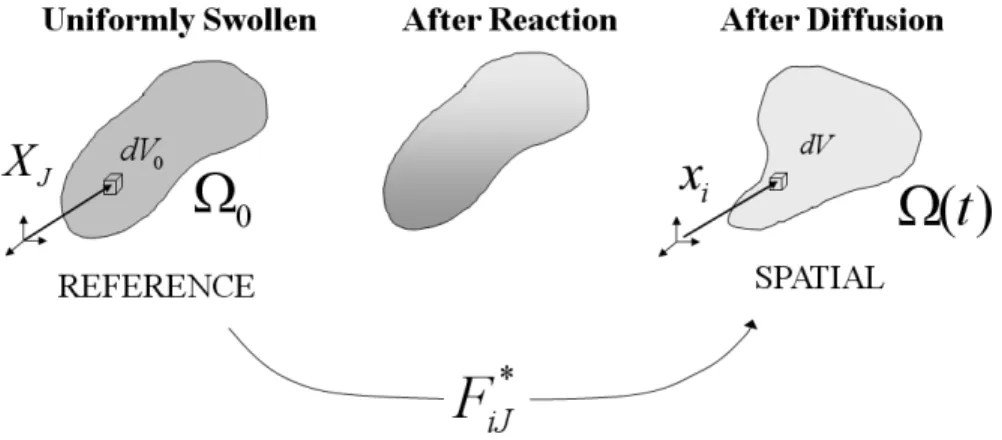
Figure 2.3: The kinematics of deformation in§2.3 (in constrast to Fig. 2.1): a swollen host network (occupying Ω0) is taken as the reference configuration; each material volumedV0is labeledXJ. This initially swollen elastomer is then exposed selectively to light, causing a spatially resolved depletion of macromer. At any point in time during the reaction–diffusion–deformation process, each material point moves to a pointxi in the spatial configuration Ω(t) and occupies a volumedV.

Let the domain of the initially-swollen system be Ω0, with each material point in the system be labeled withX (XI) relative to this new reference coordinate system. Each point also has a volume associated with it: dV0. We selectively irradiate this initially-swollen system with light and model the reaction–diffusion–deformation of the body in time. At any point in timet, we define the spatial configuration Ω(t) to be the collection of all material points mapped from the reference configuration to the current time; the initial condition for Ω(t) is Ω(0) = Ω0. In the spatial configuration, each material point occupies a positionxi and a volumedV.

From the above analysis of an initially swollen network (§2.2.2), we know that

dV0

dVd = 1 1−φ0

≡Q0. (2.3.1)

We have definedQ0as the initial swelling ratio of the system. The subsequent deformation from the initial swollen reference is denotedF∗; relative to the dry network (before macromer was introduced), the total deformation gradient is then a combination ofF∗ and the initial isotropic expansionF0=

Q1/3₀ I:

F=F∗·F0=Q 1/3 0 F

∗_{. (2.3.2)}

In terms ofF∗, the dimensionless free energy (2.2.18) is

A(F_iJ∗, φm, φN) =φmlnφm+χφmφN+ 1 2φN

Q2/3₀ trF_iJ∗F_jJ∗ −3−lnQ0−ln detFiJ∗

Since detF∗ > 1 indicates that locally the material has expanded relative to the initial swelling and detF∗<1 that the material has contracted, detF∗will be an important parameter to measure deformations in the system.

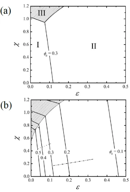
We now consider the polymerization process. In his thesis, Pape found that the modulus change due to photopolymerization of methacrylate end–capped PDMS macromer in PDMS network de-pended on volume fraction [1]. At low volume fraction (φ0 < 0.1), the effect of reaction on the modulus is better modeled by formation of nodules. This, he argued, was due to radicals first crosslinking all of the macromers in its vicinity and then capturing macromers that diffuse to it. At high volume fraction (φ0>0.2), the effect of photopolymerization of macromer on modulus was stronger, suggesting formation of a bicontinous, interpenetrating network. He was, however, un-able to prove this last hypothesis due to the paucity of models successfully predicting the modulus increase of interpenetrating PDMS networks.

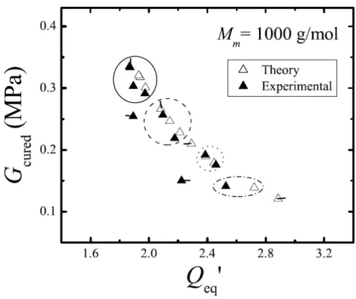
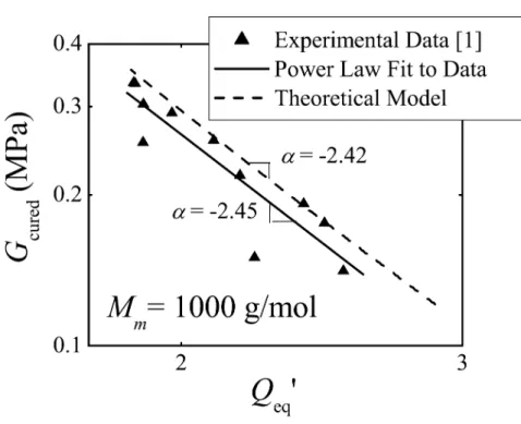
Within the same year, Yoo and co–workers characterized the mechanical and swelling properties of PDMS interpenetrating networks [31]. Although their cross–linking of the short–chain macromer proceeded through heating rather than light, they used macromers of similar length (0.8–5.7 kg/mol) and networks with similar modulus (0.7–0.21 MPa) as those used in Pape’s thesis. In order to char-acterize the materials, they measured the shear modulus of their created IPNs and compared them to theoretical work by Okumura [80]. Okumura considered two extreme models for an IPN: an equal-strain model and an equal-stress model. While the equal-equal-strain model was found to significantly overpredict the modulus of the IPNs in Yoo et al., the equal-stress model gave relatively good accord (i.e., slightly underpredicted modulus). This, coupled with the discovery that the interpenetrating networks have a similar power–law behavior (G∼Q−1.88_{) as unimodal networks (G∼Q}−1.91_{), lead} the authors to conclude that there is effective load transfer between the two networks. Thus, they concluded that the photopolymerized PDMS short–chains behaved as a bicontinuous IPN in host PDMS.

network forces the macromer–turned–network chains to retain all the original network properties before reaction, including a state of stretch present due to initial swelling with macromer. As we shall see, this theoretical artifice actually captures the mechanical behavior of the material at small volume fractions and will be shown to yield qualitatively similar results to the equal-stress model used by Yoo et al.

Although we will show that this “two-component” model is sufficient in every way to qualitatively capture experimental data (§2.3.2), we initially recognize that the different cross–linking chemistry of our small molecules from those of Yoo et al—specifically the molecular repulsion due to the methacrylate end–groups—could result in dispersed nodules, especially for lower molar masses of macromer. For this reason, we also consider an alternate model in which the macromer chains photopolymerize into discrete nodules. Following Pape’s determination that phase separation does not occur for these systems [1], we assume these nodules act as a continuous filler. We will call this second model the “three-component model” since we will consider separately free macromer, original host network, and polymerized macromer nodules. Although there are many models that can be used to represent the modulus increase due to fillers [81], we choose the Kerner equation [82]. Analgous to the equal strain and equal-stress limits proposed by Okumura, we will further-more show that the “two-component” and “three-component” models provide bounds for the cured material modulus: the two-component model underpredicts the modulus increase due to photopoly-merization, whereas the three-component model overpredicts it. As such, we assume that the actual situation is intermediate between two limiting cases: conversion of macromer into network strands and conversion of macromer into filler. We furthermore show that this model captures both the experimentally determined modulus of the PDMS materials studied by Pape and the equilibrium-swelling behavior of these materials after reaction.

2.3.1

Two-Component Model

Because there are only two components at any point in time, we note thatφN can be eliminated byφN = 1−φm. For brevity, from here on we drop the subscriptmand letφbe the volume fraction of macromer. The ratio of an element’s volume in the spatial configuration at timetto the initially dry network (§2.2) is

Q(X, t)≡ dV

dVd. (2.3.4)

This volumetric ratio Q(X, t) now differs from the familiar swelling ratio dV /dVN. The two are equal to each other in the initial spatial configuration (Q(X,0) = Q0) because no reaction has occurred (dVN =dVd). Subsequent conversion of macromer into network results in creation of new host network so that dVN > dVd. Consequently, Q can be viewed as the product of the swelling ratio (dV /dVN) and the ratio of the current amount of network to that inherited from the initial network (dVN/dVd):

Q= dV

dVd =

dV dVN

·dVN

dVd. (2.3.5)

By the definition of the volume fraction of macromer,dV /dVN = 1/(1−φ). The ratio of the current amount of network to that inherited from the initial network,θ(X, t), can be found by integrating the instantaneous rate of creation of networkrmin dV up to timet:

θ(X, t) = dVN

dVd = 1 + Z t

0

rm(X, t)

ρm0

Q(X, t)dt. (2.3.6)

The rate of reaction depends on the light flux reaching dV, the photoinitiator concentration, and the local concentration of macromer. We call the parameter θ theconversion parameter since its value completely characterizes the local, transient conversion of macromer into network. With the definition ofφandθ, (2.3.5) becomes:

Q(X, t) = θ(X, t)

1−φ(X, t). (2.3.7)

Note that (2.3.7) shows the interrelationship among the deformation (Q = detF), the chemical reaction (θ), and the diffusion of the macromer (which governs the transient volume fractionφ(X, t)). In light–adjustable lens applications, the irradiation time is short (order of min) compared to the time for re–equilibration (order of days). Reaction occurs significantly only during irradiation, decaying to zero within ≈ 5 min once the light source is turned off [1]. Since the time scale for diffusion is much greater than that for reaction, we can simplify our problem by decoupling the reaction from the diffusion–deformation process. This can be done by assuming instantaneous reaction att= 0:

rm(X, t)

ρm0

based upon plausible irradiation profiles in order to connect (2.3.8) to experiment. In the limit of instantaneous reaction (2.3.8), the conversion parameter (2.3.6) is fully specified by the extent of reactionξ(X) and the initial swelling ratio:

θ(X) = 1 + φ0 1−φ0

ξ(X). (2.3.9)

The conversion parameter is a measure of how much total macromer has reacted. Physically,θ(X) is the ratio of the local volume fraction of network immediately after the reaction to that inherited from the original network (1−φ0). This increases linearly with the product of the extent of reaction,ξ(x), and the volume fraction of macromer present when the reaction occurred, φ0. With 0 ≤φ0 ≤0.3 (the usual operating range for these swollen gels), 1≤θ≤1.4.

Since we wish to rewrite all of these expressions relative to the initially swollen configuration (as opposed to the dry network), the expression forQ(2.3.7) is simply normalized byQ0:

Q∗= detF∗ ≡ Q

Q0 = θ

∗

1−φ, (2.3.10)

where the asterisk denotes “with respect to the initially swollen state” and

θ∗= θ

Q0

= 1−(1−ξ)φ0. (2.3.11)

When the current volume fraction of macromer in a material element is greater than that present after reaction (φ(X, t)>(1−ξ)φ0), detF∗>1: macromer has diffused into the element and caused it to swell. Likewise, an element will contract (detF∗ <1) if the current volume fraction is less than that present after reaction (φ(X, t)<(1−ξ)φ0).

Since we only have two components, the system free energy is taken directly from (2.3.3):

A(F_iJ∗, φ) =φlnφ+χφ(1−φ) +1

2(1−φ)

Q2/3₀ trF_iJ∗F_jJ∗ −3−lnQ0−ln detFiJ∗

. (2.3.12)

that is, we assume that the reaction does not change the system free energy other than through depletion and creation of components. Since the set of variablesF_iJ∗ andφare not independent (see (2.3.10), the free energy (2.3.12) can be rewritten as solely a function ofF∗

iJ. This is the energy we minimize in§2.4 in order to solve global problems.

2.3.2

Region of Validity of the Two-Component Approximation

predicted shear modulus, we then illustrate that the equilibrium swelling predicted by the two-component model is also in agreement with experiment.

To determine the theoretically predicted value of G_{cured, the effective modulus of the network}

now augmented with macromer–turned–network chains, assume a sample is irradiated such that it experiences a uniform extent of reaction ξ. Although the experiments in [1] are performed at complete cure (ξ= 1), for now we considerξarbitrary to determine a general expression. Because macromer is converted uniformly, no chemical potential gradients are created and the material will not deform due to the diffusion of free macromer. With no volume change upon reaction, the volume of the material also remains unchanged (i.e., Q0 = dV0/dVd unchanged). Recall that the volume ratio of network after reaction to the dry network is the conversion parameterθ=dVN/dVd (2.3.9). Extracting any left-over macromer from the system results in a net deswelling of the material by the volume ratio

θ∗=dVN

dV0 = θ

Q0

. (2.3.13)

For the example of complete cure, dVN = dV0 and the system does not deswell at all (θ∗ = 1); arbitrary extents of reaction will then have θ∗ ≤1. Assume this deswelling occurs isotropically so that the deformation due to extraction is F_iJextract = θ∗1/3δiJ (δij the identity tensor). We then subject this cured and dried network to a shear deformation

Fδ =     

1 0 0

δ 1 0 0 0 1

    

, (2.3.14)

whereδis a small shear strain. The total deformation due to extraction and shearing isF∗=θ∗1/3Fδ. The free energy of the cured and dried (φ= 0) network under this shear becomes (2.3.12)

A(δ) =1 2 θ

2/3 _δ2_{+ 3}

−3−lnθ

!

. (2.3.15)

The derivative of the free energy