A new strain-based finite element for plane elasticity problems

City, University of London Institutional Repository

Citation:

10.1108/EC-09-2014-0181

This is the accepted version of the paper.

This version of the publication may differ from the final published

version.

Permanent repository link:

Link to published version:

Copyright and reuse: City Research Online aims to make research

outputs of City, University of London available to a wider audience.

Copyright and Moral Rights remain with the author(s) and/or copyright

holders. URLs from City Research Online may be freely distributed and

linked to.

A New Strain-Based Finite Element for Plane Elasticity Problems

ABSTRACT

In this paper, a new quadrilateral strain-based element is developed. The element has five

nodes, four at the corners as well as an internal node. Through the introduction of the internal

node, the numerical performance of the element proved to be superior to existing elements,

even though a static condensation is required. From several numerical examples, it is shown

that convergence can be achieved with the use of only a small number of finite elements. The

proposed element can be used to solve general plane elasticity problems resulting in excellent

results. The results obtained are comparable with those given by the robust element Q8.

KEY WORDS: Strain-based, Quadrilateral element, Static condensation, Analytical

integration.

1. Introduction

Since 1983, the strain-based finite element approach has been formulated by Sabir et al

[1-3] to analyze general plane elasticity problems. Among these elements is the SBRIE

(Strain-Based Rectangular In-plane Element) and SBRIE1 (Strain-(Strain-Based Rectangular In-plane

Element with An Internal Node) elements [4]. SBRIE assumes a linear variation of the direct

strains and constant variation of the shear strain, while SBRIE1 assumes a linear variation of

all three strain components. Unfortunately these elements can only be used for a regular form

with appropriate coordinates, which tend to decrease the element’s use for practical problems.

In this paper, a simple and efficient quadrilateral element having two degrees of freedom at

each node is formulated by using the concept of static condensation. It is based on the strain

approach and satisfies the equilibrium equations. However any singularity is eliminated by

the use of local axes optimally oriented. From several numerical examples, it is shown that

satisfactory results can be obtained while using only a few numbers of finite elements. This

obtained for both deflections and stresses. The results obtained are highly superior than those

obtained using the standard element Q4, and are comparable with those given by the robust

element Q8. The simplicity and efficiency of this element make it an excellent alternative for

analyzing complex civil engineering problems.

2. Description and formulation of the new element “Q4SBE5”

Figure 1a shows the geometry of the proposed element “Q4SBE5” (Strain Based

Quadrilateral Element with Four Corner Nodes and an Internal Node) and the

corresponding nodal displacements. The quadrilateral element has five nodes, four corner

nodes in addition to an internal node. Each node (i) is attributed to two degrees of freedom

(d.o.f) Ui, and Vi. Therefore, the displacement field should include ten independent constants.

The strain components at any point in the Cartesian coordinate system are expressed in

terms of the displacements as follow:

x U

x







y V

y







x V y

U

xy











For the case that the strains above equal to zero, the integration of equations (1) leads to

expressions of the form:

U = a1 - a3 y (2a)

V = a2 + a3 x (2b)

Equations (2) represent the displacement field in terms of its three rigid body displacements.

The strains in equations (1) cannot be considered independent, they are in terms of two

displacements U, V and hence must satisfy the compatibility equation. This equation can be

0 2 2 2 2 2    y x x y xy y x           (3)

Equations (2) require three independent constants (a1, a2, a3) to account for the three

components of the rigid body displacements. Therefore seven additional constants (a4,

a5,….a10) are needed to define the displacements due to straining actions. These seven

independent constants can be defined as follow:

4 5 9 6 7 10

5 7 8 9 10

a a a

a a a

a R a R + a a a

x y xy

y x

x y

x y Hy Hx

             _{    } 

Or

 

 

 

where:

 

 

1 1 v H R v v    

The strains given by equation (4) satisfy the compatibility equation (3) as well as the two-

dimensional equilibrium equations (5a, 5b):

  0

y x xy x     (5a)

 0

x y xy x     (5b)

By integrating equations (4) and substituting equations (2), we obtain the final displacement

functions:

U = a4 x+ a5 xy - a7 y2 (R +1)/2+ a8 y/2 + a9 (x2 – H y2)/2

(6a)

V= - a5 x2(R + 1)/2+ a6 y+ a7 xy + a8 x/2 + a10 (y2 – Hx2)/2 (6b)

The stiffness matrix is then calculated following well-known matrix expressions:

[Ke] = [A-1 ]T [K0 ] [A-1 ] (7a)

[K0] =

    

S T

.



where [A], [Q] and [K0] are derived in appendices A, B and C

and [D] =

      

D11 D12 0

D12 D22 0

0 0 D33

is the usual constitutive matrix





11 22 1 E D D   

 ;





. 12 1 E D   

 ; 33 2 1  E D





In this classical formulation, two problems can arise: a) the geometrical problem of distortion

of finite elements of higher degrees; and b) the problem of locking for finite elements of

relatively low degrees.

To avoid these problems, the strain-based approach with proper analytical integration is

adopted [5].

3. Evaluation of the element stiffness matrix[Ke]

The element stiffness matrix[Ke]is obtainedusing the following expression:

 

 

    

 

  

 

 A

_

K T

S T

e (8a)

[Ke] is a 10x10 matrix; however the 2 additional middle dofs are to be condensed out.

[Ke] = [A-1 ]T [K0] [A-1 ] (8b)

With:

[K0] =

    

T

S

.



Since [A] and its inverse can be evaluated numerically, the key to solving the problem

relies on the accurate evaluation of the integral in (8c). However, it is known that large

distortions typically lead to erroneous results particularly when calculating the Jacobian. In

this study, a simple expression to evaluate [K0] regardless of the degree of the polynomial of

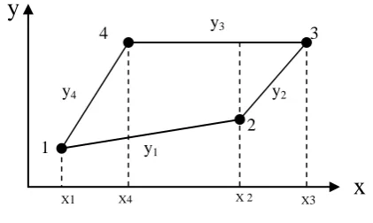
the kinematics field and the element distortion, is proposed (Fig.1b):

I = [K0] = C.x y dx.dy

s

 



where x1, x2, x3 and x4 defined in Fig. 1b are the coordinates of nodes 1, 2, 3 and 4 in

the X direction; and y1, y2, y3 and y4 are the functions of the quadrilateral sides, 1-2, 2-3, 3-4,

4-1 respectively.

The general solution of equation (9) for a quadrilateral is [5]:

I 



3

With:











m k n k i k i k j k j k

P C k a b a b x x

k C

I 1 2 1 2

2 1 . . ) ( . 1

1 (11)

The stiffness matrix is derived directly using exact and not reduced integration.

4. Validation tests

In this section, several well-established quadrilateral plane elements are compared with the

present element "Q4SBE5" through numerical test problems. The performance of elements

for distorted shapes is also tested.

The present element is compared to the following elements:

SBRIE: the strain based rectangular in-plane element [4]

SBRIE2: The strain based rectangular in-plane element with an internal node [4]

Q4: the standard four-node isoparametric element.

Q8: the standard eight -node isoparametric element.

PS5Pian and Sumihara’s four- node five-beta mixed element [6] AQ: Cook’s quadrilateral counterpart [7] of Allman’s triangle [8]

MAQ: a mixed counterpart of AQ using complete linear stress modes for all stress

components, i.e. nine stress modes are involved. Since the assumed stress space is invariant,

this element is trusted to be identical to Yunus et al’s mixed AQ [9]

Q4R the quasi- conforming counterpart of AQ proposed by Lin et al. [10]

Q4S: Mac-Neal and Harder’s refined membrane element with drilling degree of freedom [11]

07 the Sze element [12]

Q8: the Mac -Neal [13]

Allman element [8]

4.1. Bending of a cantilever beam (High order patch test)

In this test problem, the behaviour of finite elements with a significant geometrical

The problem consists of a cantilever beam having a rectangular section (l x t x h = 10 x 1 x 2),

and subjected to two nodal forces (P =1000) forming a couple (Fig. 2a).

Figures 2b and 2c show the stability, and confirm the excellent performance of the "Q4SBE5"

element regardless of the geometrical distortion (with only one element along h!). This result

can be explained because of the nature of the analytical integration carried out. The results

confirm that element Q4SBE5 passes the High Order Patch Test [14, 15].

The results of "Q4SBE5" are powerful and comparable with the exact solution. For the

standard quadrilateral element Q4, poor precision is always detected (Figures 2b and 2c).

4.2 Mac-Neal's elongated cantilever beam

In this example, the elongated cantilever beam of Mac-Neal and Harder [13] is studied

(Fig.3a). The beam has a rectangular section (6 x 2 x 1), and is subjected to a moment at the

end (M=10) as well as a load applied at its tip (P=1).

The beam is modelled by six rectangular (Fig.3a), trapezoidal (Fig.3b) and parallelogram

(Fig.3c) elements.

The results obtained using Q4SBE5 are compared with those obtained using other

well-known quadrilateral elements (Table 1).

In order to test the convergence of the Q4SBE5 element, the normalised tip deflection is

evaluated and compared with those computed using other elements in Figures (4, 5) for the

case of four different mesh configurations.

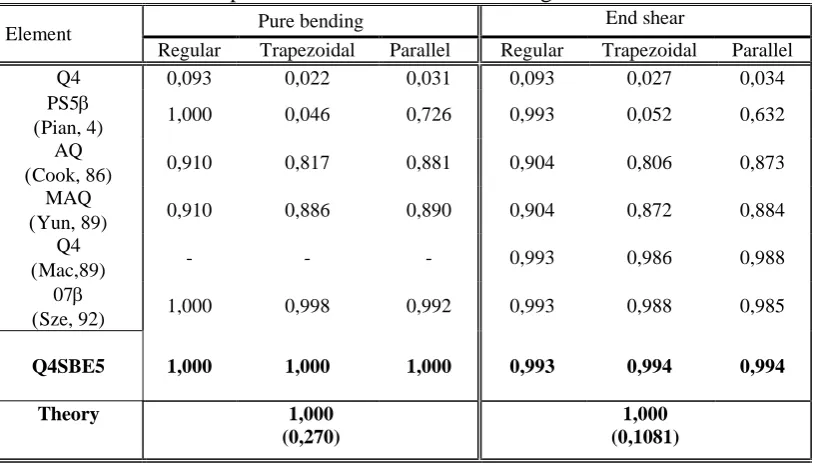
Mac-Neal [11] noted that the trapezoidal shape of membrane finite elements with four

nodes and without rotational degrees of freedom generates a locking problem, even if these

elements pass the patch-test. This problem is known as "trapezoidal locking". The results

obtained for elements Q4 and PS5(Table 1) clearly confirm the problem of trapezoidal

However, this phenomenon does not apply to finite elements based on the strain

approach. For the three meshes (Figures 3a, 3b, 3c), it is clear that the Q4SBE5 element does

not suffer from trapezoidal locking.

In conclusion, it can be confirmed that the "Q4SBE5" element is very efficient for the

case of problems dominated by bending, and that its performance remains stable with

geometrical distortions.

4.3. Allman’s cantilever beam 4.3.1. Distortion sensitivity study

In the next test problem, the vertical displacement VA at the free end of a short cantilever is

evaluated under the effect of a uniform vertical load with resultant W (Fig. 6a). This problem

is considered by many researchers as a good test to validate the efficiency of plane elements

for problems dominated by bending. The analytical solution for the vertical deflection at point

A is calculated as follow [16]:





0,3553 PL

2EH 5υ 4 3EI PL V

3

A 

 

 (12)

The results obtained for the two mesh cases (regular and distorted) are listed in Table 2.

The results in the case of the distorted mesh (Fig.6c) confirm the excellent performance of

element Q4SBE5. In this case, Q4SBE5 provides more accurate results than those of elements

PS5ß, MAQ, QR4b, 07ß and Q4 (Table 2), and is comparable with those given by the robust

element Q8, in terms of total number of degrees of freedom.

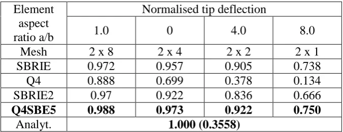
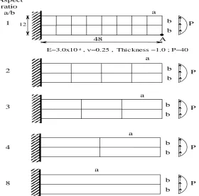
4.3.2. Aspect ratio tests for cantilever

In addition to the above test, an additional example is included here to study the sensitivity

of the present element to the variation in aspect ratio. The response of a cantilever beam to a

parabolic distributed shear applied at the tip as shown in Fig.7 is considered. From the results

requires extensive mesh refinement in order to approach the correct solution. The Q4SBE5

element however performs extremely well.

4.4. Tapered panel under end shear

This problem, proposed by Cook as a test for the accuracy of quadrilateral elements [7,

17], is another popular test problem.

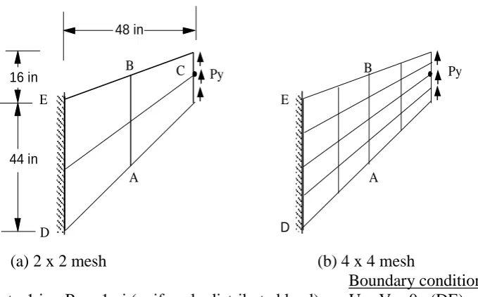
The problem consists of a tapered panel with unit thickness, and with one edge subjected to a

distributed shear load while the other edge is fully clamped (Fig. 8).

The panel is analysed by using 2 x 2 and 4 x 4 meshes (Figs 8a, 8b). The normalised

vertical deflection Vc at point C, maximum principal stress maxA at point A and minimum

principal stress minB at point B are presented in Table 4. Principal stresses at points A and B

are calculated based on the averaged stress components of the elements sharing nodes A and

B, respectively.

The results of the Q4SBE5 element are compared to those obtained using several other

quadrilateral elements. It was shown that the displacements calculated using the Q4SBE5 are

slightly better than those obtained using the other elements for both mesh cases (Table 4).

The results for deflections and principal stresses for the refined mesh (4x4) are in good

agreement to an accurate solution given in [17] using a (32x32) mesh (error 1 %).

5. Civil engineering application (Boussinesq problem, [18])

Next we examine the Boussinesq problem in the theory of linear elasticity. In this problem,

a force P is vertically applied at the center of the top surface of a semi-infinite plate. Under

the assumption of plane stress conditions, the stress component xx along the x axis is given

by the following equation [16]:

Due to the fact that infinite domains cannot be modelled using the finite element

approximations studied so far, only a finite region of the semi-infinite domain shown in Fig.9

is modelled.

Assuming homogeneity and isotropy of the material, fixed boundary conditions has been

assumed along the bottom and the right side edges. The results are shown in Fig.10 for the

case where Young’s modulus E =32000KN/mm2, Poisson’s ratio  =0.25, Thickness =10 mm

and applied force P= 100 N.

It can be concluded that the numerical results agree rather well with those of the analytical

solution.

Conclusion

The new strain based element "Q4SBE5" is proposed for the analysis of general plane

elasticity problems. It is a simple element with five nodes, four corner nodes and an internal

node, and has only two degrees of freedom per node. Several numerical examples were

studied to evaluate the performance of the strain-based approach. In general excellent results

were obtained when compared to existing elements in the literature. In addition, it can be said

that "Q4SBE5" remains stable with geometrical distortions; which is partly explained by the

nature of analytical integration carried out. It has been shown that excellent finite element

solutions can be obtained with the use of only a small number of elements making the element

References

[1] Sabir A.B., 1983. A new class of Finite Elements for plane elasticity problems, CAFEM

7th, International Conference of Structural Mechanics In Reactor Technology, Chicago.

[2] Sabir A.B., 1984. Strain based finite element analysis of shear walls. , Proceedings of the

third International Conference on Tall Building. Y.K Cheung and P.K.K. Lee, eds., Hong

Kong, pp. 447-453.

[3] Sabir A.B., 1985. A rectangular and triangular plane elasticity element with drilling

degrees of freedom, Chapter 9 in Proceeding of the 2nd International Conference on

Variational Methods in Engineering, Southampton University, Springer-Verlag, Berlin, pp.

17-25.

[4] Sabir A.B. and Sfendji A., 1995. Triangular and Rectangular plane elasticity finite

elements. Thin-walled Structures 21. pp. 225-232.

[5] Hamadi D., and Belarbi M.T., 2006. Integration solution routine to evaluate the element

stiffness matrix for distorted shapes”. Asian Journal of Civil Engineering (Building and

Housing), Vol. 7, N° 5 pp. 525 -549.

[6] Pian T.H. and Sumihara K., 1984. Rational approach for assumed stress finite elements,

International Journal of Numerical Methods in Engineering, Vol. 20, pp. 1685-1695.

[7] Cook R.D., 1986. On the Allman triangle and a related quadrilateral element, Computers

and Structure, Vol. 22, pp. 1065 -1067.

[8] Allman, D.J., 1988. Evaluation of the constant strain triangle with drilling rotations.

International Journal of Numerical Methods in Engineering. Vol. 26, pp. 2645-2655.

[9] Yunus SM.,Saigal S. and Cook R. D., 1989. On improved hybrid finite element with

rotational degrees of freedom, International Journal of Numerical Methods in Engineering,

[10] Lin H., Tang L.M. and Lu H.-X, 1990. The quasi-conforming plane element with

rotational degree of freedom. Computers and Structures Mechanics Applications. Chinese.

Vol. 7, pp. 23-31.

[11] Mac-Neal R. H. et Harder R. L., 1988. A refined four - nodded membrane element with

rotational degrees of freedom, C.S., Vol. 28, pp. 75-84.

[12] Sze K.Y., Chen W. and Cheung Y.K., 1992. An efficient quadrilateral plane element

with drilling degrees of freedom using orthogonal stress modes, Computer and Structures,

Vol. 42, N° 5, pp. 695-705.

[13] Mac-Neal R. H. and Harder R. L., 1985. A proposed standard set of problems to test

finite element accuracy, Finite Element Anal. Des. 1, pp. 3-20.

[14] Taylor R.L., Simo J.C., Zienkiewicz O.C. and Chan A.C., 1986. The patch test: A

Condition for Assessing Finite Element Convergence, International Journal of Numerical

Methods in Engineering, Vol. 22, pp. 39-62.

[15] Batoz J.L. et Dhatt G., 1990. Modélisation des structures par éléments finis, Vol. 1 :

élastiques, Editions Hermès, Paris.

[16] Timoshenko S. P., and Goodier J. N., 1970. Theory of Elasticity, 3rd Edition. Mc

Graw-Hill, New York.

[17] Bergan P.G. & Felippa C.A., A triangular membrane element with rotational degrees of

freedom, CMAME, Vol. 50, pp. 25-69, 1985.

[18] Noboru Kikuchi, Finite element methods in mechanics analysis Cambridge University

Appendices

Appendix A: Matrix [Q]

 

0 0 0 0 0 1

y x

Q x y

xR yR Hy Hx

 

 

  

     

 

Appendix B: Matrix [A]

 

2

2 2

2 2 2

2 2 2

2 2 2 2 2 2 2 2

1 0 0 0 0 0 0 0 0 0

0 1 0 0 0 0 0 0 0 0

1 0 0 0 0 0 0 0

2

( 1)

0 1 0 0 0 0

2 2 2

( 1)

1 0 0 0

2 2 2

( 1)

0 1 0 0

2 2 2

( 1)

1 0 0 0 0 0

2 2 2

0 1 0 0 0 0 0 0

2

1 0 0 ( 1) 0

2 2 4 8 4 8

0 1 0 ( 1) 0

2 8 2 4 4

a a

a R a Ha

a

b R b a Hb

b a ab

a R a b Ha

A a b ab

b R b Hb

b

b b

b a ab b b a Hb

R

a a b ab a b

Appendix C: Matrix [K0]

 

1 2 3 4 5 6

7 8 9 10 11 12

0

13 14 15 16

17 18 19 20

21 22 23

24 25

26

0

0

0

0

0

0

0

0

0

0

0

0

0

0

0

0

0

0

0

0

0

0

0

0

0

0

0

H

H

H

H

0

H

H

H

H

H

H

H

H

K

H

H

0

H

H

H

H

H

H

H

H

H

H

H

H





























 



















































11 33 11

2 11

3 3

3 12

12 12 33

2

4 12

13 22

2 2

5 11 14 22

2 2

6 12 15 12

3 3 2

7 11 33

2

8 12

2 2 2

9 33 12

1 2 1 4 2 1 3 1 2 1 1 2 2 1 1 2 2 1 3 1 2 4

H Rba D

H abD

H RHD D

H ab D

H abD

H ab D ba RHD

H ba D

H abD

H ba D H ba D

H ab D H ba D

H ab D ba R D H

H ab D

H R D D

a b

a b

























19 12 33

2 2

20 33 22

21 33

2

22 33

2

23 33

3 2 3

24 33 11

2 2

2 ₂

16 22

25 33 12

3 3 2 _{3 2 3}

17 22 33

26 33 22

2 18 33 1 3 4 1 2 1 2 1 3 1 2 ₄ 1 ₁ 3 ₃ 1 2

H ba D ab RHD

H RHD D

H abD

H ab HD

H ba HD

H ab H D ba D

ab D _{H H D D}

H ba D ab R D _{H ba H D ab D}

H ab RD

a b

a b





11 22 1 E D D   

 ;





. 12 1 E D   

 ; 33 2 1  E D    ; With:

 

 

1 1 v H R v v    

Table 1 Normalised tip deflection for Mac-Neal's elongated beam

Element Pure bending End shear

Regular Trapezoidal Parallel Regular Trapezoidal Parallel

Q4 0,093 0,022 0,031 0,093 0,027 0,034

PS5

Pian, 4) 1,000 0,046 0,726 0,993 0,052 0,632 AQ

Cook, 86) 0,910 0,817 0,881 0,904 0,806 0,873 MAQ

Yun, 89) 0,910 0,886 0,890 0,904 0,872 0,884 Q4

Mac,89) - - - 0,993 0,986 0,988

07

Sze, 92) 1,000 0,998 0,992 0,993 0,988 0,985

Q4SBE5 1,000 1,000 1,000 0,993 0,994 0,994

Theory 1,000

(0,270)

1,000 (0,1081)

Table 2 Allman's short cantilever beam, Normalised vertical displacement at point A

Formulation/ Element Mesh Normalized vertical displacement at A Allman (All., 88) Reg. 0,852

Allman (All., 88) Dist. -

PS5( Pian, 84) PS5( Pian, 84)

Reg. Dist.

0,978 0,925

AQ(Cook, 86) Reg. 0,918

AQ(Cook, 86) Dist. 0,947

MAQ(Yunus et al., 89) Reg. 0,918 MAQ(Yunus et al., 89) Dist. 0,952 QR4 (Lin. et al., 90) Reg. 0,978 QR4 (Lin. et al., 90) Dist. 0,977

07(Sze et al., 92) 07(Sze et al., 92)

Reg. Dist.

0,978 0,978

Q4 Reg. 0,679

Q4 Dist. 0,596

Q8 (Mac., 88) Reg. 0,985

Q8 (Mac., 88) Dist. 0,994

Q4SBE5 Reg. 0,983

Q4SBE5 Dist. 0,995

Exact solution (Timoshenko, 1970) 1,000

Table 3 Normalized deflection at point A, of a cantilever beam under a tip load

Element aspect ratio a/b

Normalised tip deflection

1.0 0 4.0 8.0

Mesh 2 x 8 2 x 4 2 x 2 2 x 1

SBRIE 0.972 0.957 0.905 0.738

Q4 0.888 0.699 0.378 0.134

SBRIE2 0.97 0.922 0.836 0.666

Q4SBE5 0.988 0.973 0.922 0.750

Table 4 Normalised prediction for tapered panel under end shear

Element model 2 x 2 mesh 4 x 4 mesh VC maxA minB VC maxA minB

Q4 0,496 0,437 0,533 0,766 0,756 0,719 AQ

(Coo., 86) 0,890 0,780 0,900 0,965 0,936 1,010 Ref. (All., 88) 0,848 0,771 0,856 0,953 0,956 0,997

FRQ

(Aya., 93) 0,914 0,741 0,775 0,973 0,932 0,985 PS5

Pian, 84) 0,884 0,786 0,771 0,963 0,950 0,924 MAQ

Yun, 89) 0,890 0,779 0,886 0,965 0,941 0,967 QR4

(Lin, 90) 0,941 0,879 1,059 0,980 0,990 0,997 Ref. (Ber., 85) 0,852 0,720 0,898 0,938 0,902 0,849

Ref.(Ibr., 90) 0,865 - - 0,962 - - Ref. (Sim., 89) 0,884 - - 0,963 - -

07

Sze, 92) 0,945 0,835 1,069 0,981 0,982 1,012

Q4SBE5 1,0652 1,508 1,171 1,011 1,004 0,992

32 x 32 mesh

Ref. Ber., 85

1,000 (23,90)

1,000 (0,236)

1,000 (-0,201)

1,000 (23,90)

1,000 (0,236)

Fig.1a: Co-ordinates and nodal points for the element” Q4SBE5

Fig.1b: Quadrilateral element

X4 X 2 _X3

X1

y4

3

y1

y

x

y2

y3

4

2

1

5+e 5-e

B

A 1000

1000 E = 1500 _{ = 0,25}

t = 1,0 U = 0

U = V = 0 2

a) Pure Bending of a Cantilever beam; Data and Meshes

b) Vertical Displacement at Point A. Normalised results

c) Normal stress at Point B. Normalised results

Fig.2. Pure bending of a cantilever beam

VA

No

rm

alis

ed

resu

lts

No

rm

alis

ed

r

esu

lts

0 0,2 0,4 0,6 0,8 1 1,2

0 1 2 3 4 5 _e 6

Q4SBE5 Q4 Exact

0 0,2 0,4 0,6 0,8 1 1,2

0 1 2 3 4 5 _e 6

Fig.3 Mac-Neal's elongated beam subject to (1) end shear and (2) end bending.

case

10 0 ,2

10

10 ( 2 ) ( 1 )

1

1 1 1 1 1 1

a) Regul ar Shape Elements

45 ° 45 °

1 b) Trapezoidal Shape Elements

Data: E = 107, ν = 0,3, L = 6, t = 0,1 45 °

1 c) Parallelogram Shape Elements

NEL= Number of elements

Fig.4 Convergence Curves for deflection at point A

Mac- Neal’s cantilever beam under pure bending

Def

lectio

n

at

p

o

in

t A

0

0,05 0,1 0,15 0,2 0,25

0,3

0 2 4 6 8 10 12_NEL 14

Fig.5Convergence Curves for deflection at point A Mac-Neal’s cantilever beam under end shear

Def

lectio

n

at

p

o

in

t A

0 0,02 0,04 0,06 0,08 0,1 0,12

0 2 4 6 8 10 12 _NEL 14

Fig.6 Allman's cantilever beam; Data and mesh

a A H

16 4 8 20

12 12 12 12

E = 3.104 Ksi, =0,25, t=1,0 in

W= 40 K, L = 48 in, H =12 in W

b/ Regular mesh

L

b

a/ Cantilever beam. Data

a b b

b b

b b

b b

b b a

a

a

a

P Aspect

ratio a/b

1

2

3

4

8

P

P

P

P 48

12

E=3.0x104 _, _{Thickness =1.0 ; P=40}

A

Fig.7 Cantilever beam subjected to parabolically distributed shear

C

E

D

B

A

Py

E

D

B

A

Py 48 in

16 in

44 in

(a) 2 x 2 mesh (b) 4 x 4 mesh

Boundary conditions: Thickness t =1 in; Py = 1 pi (uniformly distributed load) U = V = 0 (DE)

Fig.8 Tapered panel subjected to end shear; data and meshes

Fig.9 Domain for Boussinesq problem  r,

y

x

Applied Force P=100 N

10 mm 10 mm

Fig.10.Stress σxx along x Axis (θ=900)

σ

(N/m

m

2 )

-350

-300

-250

-200

-150

-100

-50

0

0 1 2 3 4 5 6 7 8 9 10 11

X(mm)