This is a repository copy of Bayesian System Identification of Dynamical Systems using
Reversible Jump Markov Chain Monte Carlo.
White Rose Research Online URL for this paper:
http://eprints.whiterose.ac.uk/81832/
Proceedings Paper:
Tiboaca, D., Green, P.L., Barthorpe, R.J. et al. (1 more author) (2014) Bayesian System
Identification of Dynamical Systems using Reversible Jump Markov Chain Monte Carlo. In:
Proceedings of IMAC XXXII, Conference and Exposition on Structural Dynamics. IMAC
XXXII, Conference and Exposition on Structural Dynamics, 3-6 February 2014, Orlando,
Florida USA. .
[email protected] https://eprints.whiterose.ac.uk/
Reuse
Unless indicated otherwise, fulltext items are protected by copyright with all rights reserved. The copyright exception in section 29 of the Copyright, Designs and Patents Act 1988 allows the making of a single copy solely for the purpose of non-commercial research or private study within the limits of fair dealing. The publisher or other rights-holder may allow further reproduction and re-use of this version - refer to the White Rose Research Online record for this item. Where records identify the publisher as the copyright holder, users can verify any specific terms of use on the publisher’s website.
Takedown
If you consider content in White Rose Research Online to be in breach of UK law, please notify us by
Bayesian System Identification of Dynamical Systems using
Reversible Jump Markov Chain Monte Carlo
D.Tiboaca, P.L.Green, R.J.Barthorpe, K.Worden
University of Sheffield
Department of Mechanical Engineering, Sir Frederick Mappin Building, Mappin Street, S1 3JD
email: [email protected]
Abstract
The purpose of this contribution is to illustrate the potential of Reversible Jump Markov Chain Monte Carlo (RJMCMC) methods for nonlinear system identification. Markov Chain Monte Carlo (MCMC) sampling methods have come to be viewed as a standard tool for tackling the issue of parameter estimation using Bayesian inference. A limitation of standard MCMC approaches is that they are not suited to tackling the issue of model selection. RJMCMC offers a powerful extension to standard MCMC approaches in that it allows parameter estimation and model selection to be addressed simultaneously. This is made possible by the fact that the RJMCMC algorithm is able to jump between parameter spaces of varying dimension. In this paper the background theory to the RJMCMC algorithm is introduced. Comparison is made to a standard MCMC approach.
Key words: Nonlinear Dynamics, System Identification, Bayesian Inference, MCMC, RJMCMC
1
Introduction
Since their invention in 1953, Markov Chain Monte Carlo (MCMC) sampling methods have been used in many research areas where they have proved their capacity of sampling from probability density functions (PDFs) with complex geometries. In the domain of system identification (SID), MCMC has been exten-sively used as a tool for parameter estimation. MCMC sampling methods are part of a group of algorithms that, through the use of generated samples from geometrically complicated PDFs, can be implemented to estimate the parameters on which a system depends. Because they make use of PDFs, MCMC algorithms have proven to work extremely well within a Bayesian framework. By joining these two concepts, one can conduct SID for either linear or nonlinear models efficiently. This is of great interest in structural dynamics, at a time when nonlinear models still remain difficult to identify and understand.
The aim of this contribution is to give a better understanding of the RJMCMC algorithm and its appli-cation in system identifiappli-cation. A comparison is made between the Metropolis-Hastings (one of the MCMC samplers) algorithm and the RJMCMC algorithm in order to demonstrate the advantages of the later in model selection. The detailed balance principle is explained and it is proven that it is respected by both Metropolis-Hastings and RJMCMC algorithms. The power of RJMCMC is demonstrated through its ability of dealing efficiently with model selection and parameter estimation (simultaneously) for both linear and nonlinear models.
a continuum of optimum parameter vectors). Paper [1] tackles the problems of uncertainty and reliability as well. Rather than selecting the model considering the data as was done in previous work with SID, the paper proposes a predictive approach which puts together all possible models according to their probability of being the right choice, given the data. Other work worth mentioning in the fields of Bayesian Inference and MCMC was conducted by Worden and Hensman [2] and Green and Worden [3]. The work discussed in [2] is concerned with offering a Bayesian framework to nonlinear system identification (i.e. parameter estimation and model selection). The importance of the work presented was particularly related to the use of Bayesian inference and MCMC sampling methods on nonlinear systems. Two different systems were simulated to demonstrate the validity of the approach: the Duffing Oscillator and the Bouc-Wen hysteresis model. The Metropolis-Hastings MCMC method was used to generate samples, demonstrate parameter correlations and help in model selection. [3] tackles the problems of parameter estimation and also model selection for an existing nonlinear system (i.e. the data used was from a real system rather than a simulated one) using a Bayesian approach through MCMC methods. The nonlinearities introduced were of a Duffing kind (i.e. cubic stiffness) and friction type (using viscous, Coulomb, hyperbolic tangent and LuGre friction models). Other work on MCMC can be found by the interested reader in [4].
Even though MCMC is an impressive approach when it comes to parameter estimation, when system identification is conducted, there is also the need to tackle the model selection issue. As most MCMC methods do not cover model selection, Green [5] introduced Reversible Jump Markov chain Monte Carlo (RJMCMC), a tool that covers both problems of system identification, i.e parameter estimation and model selection. In the past few years there has been a lot of research conducted in model selection using Green’ s [5] RJMCMC algorithm. Some mentionable work with RJMCMC was done by Dellaportas et al [6], where they employed RJMCMC on the problems of logistic regression and simulated regression, using a Gibbs sampler, which is an alternative MCMC sampling method used for parameter estimation. In order to demonstrate the computational efficiency of the algorithm on Nonlinear Autoregressive Moving Average with eXogenous(NARMAX) input models, Baldacchino,et al [7] presented a comparison between the for-ward regression method and the RJMCMC method. A thorough explanation of the RJMCMC method can be found in [8] where Green, the developer of the algorithm, provides further explanations of the method. There is also some work done in signal processing using RJMCMC and it can be found in [9] and [10].
The current paper aims to introduce the RJMCMC algorithm in the context of structural dynamics, explaining how the algorithm works and how it can be related to one particular sampler of MCMC, the Metropolis-Hastings algorithm. The paper is structured as follows. Section 2 will be an introduction to Bayesian inference and its relevance in system identification. Section 3 introduces the background of MCMC sampling methods, in particular the Metropolis-Hastings sampler, together with its importance in SID. Section 4 is concerned with describing background on RJMCMC and linking RJMCMC with the Metropolis-Hastings algorithm (in the context of structural dynamics). The last section, Section 5, gives insight on future work and concludes the present contribution.
2
Bayesian Inference
When it comes to structural dynamics, one of the classes of interest is system identification (SID). The main concerns of SID are parameter estimation (every system will depend on a set of parameters) and model se-lection. Unfortunately, when it comes to identifying systems, uncertainties will inevitably arise. This allows one to know a system only to a probabilistic extent. Probability helps to extract order from randomness and one cannot talk about probability without making use of the concept of a probability distribution. One of the conditions of probability theory is that the probability distribution must always integrate to 1.
In this case, the random variables one is interested in are the parameters of the system of interest. There has been defined at this point a set of parameters,θ={θ1, θ2, ..., θR} which needed to be estimated.
parameter estimation. Bayes’ theorem states that the posterior will equal the product of the likelihood and prior, divided by the evidence:
P(θ|D, M) =P(D|θ, M)P(θ|M)
P(D|M) (1)
The posterior,P(θ|D, M), is the probability of the parametersθafter one has seen some measured data,
D, the data being whatever response was measured. The evidence,P(D|M), acts as a normalising constant and it ensures the area under the posterior is unity, as required by probability theory. The prior,P(θ|M), is the probability assigned to the parameters before one has seen the data. It represents one’s knowledge about the system from previous experience. For further reading about priors, relevant information can be found in [11].
The likelihood, P(D|θ, M), is the probability of seeing the data given the selected model and the
pa-rameters that one wishes to estimate. It is typically viewed as the most important function (in spite of its form, the likelihood is not a probability distribution when the data is constant andθ is varied) to evaluate
in Bayes’ theorem. Analytical evaluation of the likelihood term is often hard to achieve when one has a set of parameters.
Numerical evaluation of the evidence is not feasible once the number of parameters is bigger than 3, as it gets computationally expensive. MCMC algorithms typically allow one to generate samples without having to evaluate the evidence term.
3
MCMC sampling methods
Markov Chain Monte Carlo methods are sampling algorithms that employ the use of random variables. Their purpose is to solve the issues of generating samples from a probability distribution with complex geometry. MCMC algorithms work by creating a Markov chain of parameter samples,θi, whose stationary
distribution is equal to the desired, target distribution. The desired distribution is the posterior.
There are many MCMC methods, each with their own advantages and disadvantages, but for the time being and for the purpose of this paper only, the Metropolis-Hastings (MH) method will be explained as it has been the most employed for parameter estimation. One begins by choosing a target density, π(θ),
(which in this case will be the posterior parameter distribution). Then, one chooses a proposal density,
Q(θ′|θ) ,which is often a multivariate Gaussian (multivariate because one must not forget thatθ is a set of
parameters).The next step is to generate a sample θ′ from the proposal density,Q(θ′|θ) and a quantity α
is built (as shown below). This is known as the Metropolis acceptance rule and it is used to decide if the proposed sample will be accepted or if the chain remains at the current state.
To generate N parameter samples using the MH algorithm [12]:
Initialize
forn= 1 :N do
Generateθ′ f rom Q(θ′|θ) ;
Calculate α = π(θ′)Q(θ(
n)|θ′)
π(θ(n))Q(θ′|θ(n)) ; if α ≥1then
−new state accepted;
θ(n+1) =θ′ ;
else
−new state accepted with probability α;
θ(n+1) =θ(n);
end if end for
For further insights into the Metropolis-Hastings algorithm, the interested reader is directed to [13].
that may explain the physical behaviour of the experimental system. Even if the models are of the same dimension, they could be differently parameterized. If one takes into consideration that the models might be of different dimensions as well, the issue is amplified. RJMCMC can handle model selection.
4
RJMCMC
With Reversible Jump MCMC one can address parameter estimation and model selection simultaneously. The way the algorithm works is that it can move/’jump’ between parameter spaces of different dimension. The vector set of parameters is not fixed to each model; it can vary in both length and values. Reversible Jump MCMC is capable of ’jumping’ from one model to the other and select the most likely model while generating parameter samples for that particular type of system.
In the set of models,M, the models will be arranged in the order of their complexity; in this particular
case a more complex model is defined as one with more parameters.
There are three main moves in the RJMCMC method:
• Birth move - which implies that if the birth move condition is satisfied, the algorithm moves to a model with an additional parameter;
• Death move - which implies that if the death move condition is satisfied, the algorithm ’jumps’ to a model with one less parameter;
• Update move - which implies that if neither the birth move condition nor death move condition were satisfied, the algorithm remains within the same model and the use of the normal MH algorithm is employed, as presented before, for parameter estimation.
The birth move will be randomly attempted with probabilitybl, where :
bl=pmin
1,P(l+ 1) P(l)
(2)
The death move will be randomly attempted with probabilitydl, where:
dl+1=pmin
1, P(l)
P(l+ 1)
(3)
Lastly, the update move will be randomly attempted with probability ul, so that
bl+dl+ul= 1 (4)
The variable l is an indicator of the current model, the variable p adjusts the proportion of the up-date move in relation with the birth and death moves, and the probabilities, P(l) andP(l+ 1), are prior probabilities of the models at iterationlandl+ 1 respectively.
By using equations 2 and 3 one can see that:
blP(l)
dl+1P(l+ 1)
= 1 (5)
It is assumed at this point that one has a set of two potential models of a SDOF system,M =
{ M(1), M(2)} ,where model M(1) has one unknown, θ(1), while model M(2) has two unknown
parame-ters,{θ(2)1 , θ(2)2 }.
The first model is described by the following equation:
my¨+cy˙+k(1)y=F (6)
my¨+cy˙+k(2)y+k3(2)y3=F (7) wherey∈Dis the data available for the two models andF ∈Dis the excitation applied to each system.
Fig. 1is a possible representation of the two models. In the context of the two equations of motion and the models presented above, the massmis assumed known as well as the damping coefficient,c, whilek(1)=θ(1)1
andk(2) =θ(2) 1 ,k
(2) 3 =θ
(2)
2 are the unknown parameters.
Fig. 1: (a) Linear system, (b) Nonlinear system of Duffing type
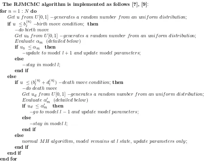
The RJMCMC algorithm is implemented as follows [7], [9]:
forn= 1 :N do
Get u f rom U[0,1]−generates a random number f rom an unif orm distribution;
if u ≤b(ln)−birth move condition; then
−do birth move
Get ub f rom U[0,1]−generates a random number f rom an unif orm distribution;
Evaluate αm (detailed below)
if ub ≤αm then
−update to model l+ 1 and update model parameters;
else
−stay in model l;
end if else
if u ≤(b(ln)+d
(n)
l )−death move condition;then
−do death move
Get ud f rom U[0,1]−generates a random number f rom an unif orm distribution;
Evaluate α′
m (detailed below)
if ud ≤α′m then
−go to model l−1and update model parameters;
else
−stay in model l;
end if else
normal M H algorithm, model remains at l state, update parameters only;
end if end if end for
The acceptance probabilities of the birth and death moves, respectively αm, α′m, will be evaluated in
[image:6.612.119.460.149.313.2] [image:6.612.64.484.341.669.2]With the models introduced at the beginning of this section one notices a difference in dimensions: the first model has only one unknown parameter while the second model has two unknown parameters. This makes it a good point to introduce the concept of detailed balance, a principle that must be respected in order for MCMC or RJMCMC methods to generate samples from the target PDF. This is simpler to demonstrate for MH as the dimension space remains the same. With RJMCMC it becomes harder to maintain because the dimension space varies.
4.1
Detailed Balance and MH Sampler
The most important aspect of MCMC methods is that detailed balance is respected. In general terms, de-tailed balance states that at equilibrium every process should be balanced out by its reverse process. In the context of MH sampling, detailed balance ensures that ergodicity and a limiting distribution are respected [5]. Further details on ergodicity and limiting distributions can be found in [12].
The following analysis will make use of the concept of mappings, which are functionals that can relate one state to another [14]. In the current work, the mappingh:θ →θ′ is defined as the path from θ toθ′
with its inverse,h−1being defined as the path fromθ′ toθ. Detailed balance states that, for the standard
Metropolis-Hastings algorithm, for a modelM that depends on two parameters, i.e. θ={ θ1, θ2}
π(θ)T(θ→θ′) =π(θ′)T(θ′→θ) (8)
The above equation is true no matter what path one chooses to take fromθtoθ′, which in mathematical
terms translates into:
Z
π(θ)T(θ→θ′) dθ=
Z
π(θ′)T(θ′ →θ) dθ (9)
Putting the above equation in the extended form, results in the following equation:
Z Z
π(θ)q(θ′|θ′)α(θ→θ′) dθ1dθ2=
Z Z
π(θ′)q(θ|θ′α)(θ′ →θ) dθ1′dθ2′ (10)
Assuming that one had a mappingh,h:θ→θ′, then a relationship can be expressed using the Jacobian
matrix, once the substitution rule was applied :
dθ′1dθ′2=
∂ (θ′
1, θ2′) ∂ (θ1, θ2)
dθ1dθ2 (11)
where
∂ (θ′
1, θ′2) ∂ (θ1, θ2)
= det
"∂θ′
1 ∂θ1 ∂θ′ 1 ∂θ2 ∂θ′ 2 ∂θ1 ∂θ′ 2 ∂θ2 # (12)
So, replacing into the previous equation gives the new expression for detailed balance:
π(θ)q(θ′|θ)α(θ→θ′) =π(θ′)q(θ|θ′)α(θ′ →θ)
∂ (θ′
1, θ2′) ∂ (θ1, θ2)
(13)
Assuming that the mapping h exists, one can look into its form. One could choose to propose new parametersθ1′ andθ2′ using Gaussian distributions centred around the current parameters:
θ′1=θ1+a (14)
and
θ′2=θ2+b (15)
θ′ 1 θ′ 2 = a b + θ1 θ2 (16)
Calculating the Jacobian using equations 14 and 15 one finds that:
∂θ′
1 ∂θ1
= 1,∂θ
′
1 ∂θ2
= 0,∂θ
′
2 ∂θ1
= 0,∂θ
′
2 ∂θ2
= 1 (17)
This means that the determinant becomes equal to 1, no matter what the generated values of a and
b might be. The above explanations will hold and prove detailed balance when using the MH algorithm because the dimension matching requirement is met.
4.2
Detailed Balance and RJMCMC
Detailed balance, when it comes to RJMCMC, gets more complicated to evaluate because each variable is part of a space of different dimension. This implies that one cannot be sure that the space dimension of the right hand side is necessarily equal to the space dimension of the left hand side.
Going back to the two models presented at the beginning of the section, one assumes that the mass m
is known and that these will be damped, forced systems with known damping coefficients c. This implies that modelM(1)is dependent only on the unknown stiffnessk(1)=θ
1and that the nonlinear modelM(2)is
dependent on the stiffnessk(2)=θ′
1and the cubic stiffness that introduces the nonlinear element,k (2) 3 =θ
′ 2.
One can see that there is a mismatch in dimensions. Jumping from model M(1) to model M(2) is not
possible at this point in time as the detailed balance principle is not respected (a space of dimension 1 does not equal a space of dimension 2). In order to match the dimensions one must make modelM(1) depend on
an additional parameterub, such that both spaces are of the same dimension. The parameterub influences
the choice ofθ2′ . This was referred by Green [5] as ’dimension matching’. Writing the detailed balance for the two models for RJMCMC algorithm, one has:
π(θ)q(θ′|θ)α(θ→θ′) =π(θ′)q(θ|θ′)α(θ′→θ)
∂ (k(2), k3(2))
∂ (k(1), u
b) (18)
where, in this case,θ={k(1), u
b} andθ′ ={ k(2), k(2)3 } .
Again, the mapping will be of the following form:
θ′ 1 θ′ 2 = a b + θ1 ub (19)
which assures that the Jacobian, as before, will be unity, no matter the values of aorb.
Matching the dimensions above proved that the chosen mapping h is differentiable. Remember from before that the detailed balance only holds if the chosen mapping is differentiable and unique. The mapping was proven to be differentiable but one has to prove that it is (1−1). This is very straightforward. There is a theorem, called the inverse function theorem, that confirms that as long as the Jacobian at a pointθis nonzero (which was proved to be true, the Jacobian is 1 all the time) then the mappinghis unique [14].
The work presented until this point demonstrated detailed balance for the RJMCMC algorithm. This means that one can evaluate the acceptance probabilities of move,αm() andα′m() , on which the conditions
of birth and death depend on. The acceptance probability of the birth move can be evaluated as:
αm(θl→θl′) = min
1, π(θ
′
l)
π(θl)g(ub)
(20)
where all the values are known or can be estimated and one can notice that the Jacobian is not included as it is always equal to 1, no matter the conditions.
The acceptance probability of the birth move can be written also as:
where rm is the ratio of move and is computed as:
rm=
π(θ′l)
π(θl)g(ub)
(22)
The acceptance probability of the death move can be evaluated as:
α′m(θl →θl′) = min
1, r−m1 (23)
At this point one gets a better grasp of the concepts needed to understand the RJMCMC algorithm and the mathematical tools for implementing it with either real or simulated data.
5
Conclusions
This current contribution introduced the RJMCMC algorithm and provided a comparison between the most widely used MCMC sampling method, the MH, and RJMCMC. While the first one only covers parameter estimation, the RJMCMC method is used to cover both issues of SID, parameter estimation and model selection.
As part of future work on the subject, the authors plan to introduce the RJMCMC in the context of nonlinear dynamical systems and its applicability will be demonstrated through application to an exemplar system for which alternative models exist.
References
[1] L.J. Beck S-K. Au. Bayesian updating of structural models and reliability using markov chain monte carlo simulation. Journal of Engineering Mechanics, 391:128–380, 2002.
[2] K. Worden J.J. Hensman. Parameter estimation and model selection for a class of hysteretic systems using bayesian inference. Mechanical Systems and Signal Processing, 32:153–169, 2012.
[3] P.L. Green K. Worden. Modelling friction in a nonlinear dynamic system via bayesian inference. IMAC XXXI Proceedings, 2013.
[4] B.P. Carlin S. Chib. Bayesian model choice via markov chain monte carlo methods. Journal of the Royal Statistical Society, Series B (Methodological), 57:473–484, 1995.
[5] P.J. Green. Reversible jump markov chain monte carlo computation and bayesian model determination.
Biometrika, 82:711–732, 1995.
[6] P. Dellaportas I. Ntzoufras, J.J. Forster. On bayesian model and variable selection using mcmc.Statistics and Computing, 36:12–27, 2002.
[7] T. Baldacchino V. Kadirkamanathan, S.R. Anderson. Computational system identification for bayesian narmax modelling. Automatica, 49:2641–2651, 2013.
[8] P.J. Green D.I. Hastie. Model choice using reversible jump markov chain monte carlo. Statistica Neerlandica, pages 309–338, 2012.
[9] C. Andrieu A. Doucet. Joint bayesian model selection and estimation of noisy sinusoids via reversible jump mcmc. IEEE Transactions on Signal Processing, 1999.
[10] C. Andrieu A. Doucet, P.M. Djuric. Model selection by mcmc computation.Signal Processing, 81:19–37, 2001.
[11] S. Geinitz. Prior covariance choices and the g prior. 2009.
[13] S. Chib E. Greenberg. Understanding the metropolis-hastings algorithm. The American Statistician, 1995.