This is a repository copy of
How Can Subsampling Reduce Complexity in Sequential
MCMC Methods and Deal with Big Data in Target Tracking?
.
White Rose Research Online URL for this paper:
http://eprints.whiterose.ac.uk/127881/
Version: Accepted Version
Proceedings Paper:
De Freitas, A., Septier, F., Mihaylova, L. orcid.org/0000-0001-5856-2223 et al. (1 more
author) (2015) How Can Subsampling Reduce Complexity in Sequential MCMC Methods
and Deal with Big Data in Target Tracking? In: Proceedings of the 18th International
Conference on Information Fusion. 18th International Conference on Information Fusion,
06-09 Jul 2015, Washington DC, USA. IEEE , pp. 134-141.
[email protected] https://eprints.whiterose.ac.uk/
Reuse
Unless indicated otherwise, fulltext items are protected by copyright with all rights reserved. The copyright exception in section 29 of the Copyright, Designs and Patents Act 1988 allows the making of a single copy solely for the purpose of non-commercial research or private study within the limits of fair dealing. The publisher or other rights-holder may allow further reproduction and re-use of this version - refer to the White Rose Research Online record for this item. Where records identify the publisher as the copyright holder, users can verify any specific terms of use on the publisher’s website.
Takedown
If you consider content in White Rose Research Online to be in breach of UK law, please notify us by
arXiv:1507.08526v1 [stat.CO] 30 Jul 2015
How Can Subsampling Reduce Complexity in
Sequential MCMC Methods and Deal with Big
Data in Target Tracking?
Allan De Freitas
∗, Franc¸ois Septier
§, Lyudmila Mihaylova
∗, Simon Godsill
♮∗Department of Automatic Control and Systems Engineering, University of Sheffield, United Kingdom
§ Institute Mines Telecom/Telecom Lille, CRIStAL UMR CNRS 9189, France
♮Department of Engineering, Cambridge University, CB 1PZ, United Kingdom
Emails: [email protected], [email protected], [email protected], [email protected]
Abstract—Target tracking faces the challenge in coping with
large volumes of data which requires efficient methods for real time applications. The complexity considered in this paper is when there is a large number of measurements which are required to be processed at each time step. Sequential Markov chain Monte Carlo (MCMC) has been shown to be a promising approach to target tracking in complex environments, especially when dealing with clutter. However, a large number of mea-surements usually results in large processing requirements. This paper goes beyond the current state-of-the-art and presents a novel Sequential MCMC approach that can overcome this chal-lenge through adaptively subsampling the set of measurements. Instead of using the whole large volume of available data, the proposed algorithm performs a trade off between the number of measurements to be used and the desired accuracy of the estimates to be obtained in the presence of clutter. We show results with large improvements in processing time, more than 40 % with a negligible loss in tracking performance, compared with the solution without subsampling.
I. INTRODUCTION
Flooded with data, richly provided by electronic sensors, the current monitoring systems face the problem of being able to process the data and monitor the phenomenon of interest at the same time. In this paper we consider the problem of target tracking in large volumes of data. There is a wealth of algorithms that can provide sequential estimation of the states of the target, e.g. for details see [1], [2]. In a Bayesian frame-work, the posterior distribution can be iteratively computed. However, analytically this can be achieved only when the state space model is linear and perturbed by a Gaussian noise. In this case the solution is referred to as the Kalman Filter. There are a large number of techniques which overcome the limitations of the Kalman filter based on the sequential Monte Carlo (SMC) methodology. The seminal work on SMC in target tracking was presented in [3] which was also referred to as the bootstrap particle filter (PF). The bootstrap PF and many variants thereof, broadly referred to as PFs, are commonly favoured techniques in a wide variety of applications due to the filters ability to handle non-linear state space models and/or state space models perturbed by non-Gaussian noise. However, the PF is not void of challenges. Some of the difficulties faced by PFs includes weight degeneracy and
sample impoverishment. Although there are variants of the PF which have been proposed to alleviate these issues [4], [5], the PF is still susceptible to degeneracy, and these difficulties are more profound when tracking complex systems.
Markov chain Monte Carlo (MCMC) techniques are a powerful set of algorithms for sampling from a probabil-ity distribution. MCMC tecnhiques, such as the Metropolis Hastings (MH) algorithm, have been predominantly used in applications requiring static inference [6]. Recently there has been considerable interest in extending these techniques to sequentially updating the posterior distribution [7], [8]. Se-quential MCMC has shown promising results for complex systems. The largest hindrance being long processing times which could limit usage in applications required to run in real time. There have also been several algorithms [9], [10], [11] which have been proposed to help reduce computational complexities when performing static inference with MCMC techniques on large datasets.
In this paper we propose a novel technique which results in an efficient sequential MCMC algorithm when applied in com-plex systems consisting of a large number of measurements. This is achieved through the combination of sequential infer-ence and adaptive subsampling of the measurements at each time step. We show how the proposed adaptive subsampling sequential MCMC algorithm can be applied to target tracking and illustrate the computational savings it affords.
II. PROBLEMFORMULATION
Target tracking of a complex system can be considered as sequential state estimation with multiple measurements. This can be achieved in a Bayesian framework by sequentially computing the filtering posterior distributionp(xk|z1:k)where
xk∈Rnx is the state vector at timet
k withk= 1, ..., T ∈N,
and z1:k = {z1, ...,zk}, represents all the measurements
received up till time tk. The measurements received at each
time tk are represented by a set zk = {z1k, ...,z Mk
k }, where
Mk is the total number of measurements and zik∈Rnz. The
on
p(xk|z1:k)∝
Z
p(zk|xk)p(xk|xk−1)p(xk−1|z1:k−1)dxk−1,
(1) where p(zk|xk) is referred to as the likelihood probability
density function (pdf), and p(xk|xk−1) is referred to as the
state transition pdf. An analytical solution to (1) is typically intractable when the state space model is characterised by non-linearities and/or non-Gaussian noise.
A. Sequential Markov Chain Monte Carlo
MCMC methods work by constructing a Markov chain with a desired distribution as the equilibrium distribution. A common MCMC technique used to obtain samples from the equilibrium distribution, π(x), is the MH algorithm. This is achieved by first generating a sample from a known proposal distribution x∗ ∼ q(· |xm−1). The proposed sample is ac-cepted as the current state of the chain, xm, if the following condition is satisfied
u < π(x
∗)q(xm−1|x∗)
π(xm−1)q(x∗|xm−1), (2)
whereurepresents a sample from a uniform random variable
u ∼ U[0,1]. Using Bayes’ rule and assuming that there are
M conditionally independent measurements,zi, results in the further expansion of this expression
u < p(x
∗)q(xm−1|x∗)
p(xm−1)q(x∗|xm−1) M
Y
i=1
p(zi|x∗)
p(zi|xm−1). (3)
The previous state of the chain is stored as the current state,
xm =xm−1, when the proposed sample does not meet this criterion. We further manipulate this expression into a form with the likelihood isolated:
log
up(x
m−1)q(x∗|xm−1)
p(x∗)q(xm−1|x∗)
<
M
X
i=1
log
p(zi|x∗)
p(zi|xm−1)
.
(4) In [7] it was proposed to use MCMC methods, specifically the MH algorithm, to target the filtering posterior distribution in (1) as the equilibrium distribution. This allows for the iterative update of an approximation of the filtering posterior distribution by representing p(xk−1|z1:k−1) with a set of
unweighted particles,
p(xk−1|z1:k−1)≈ 1
Np Np
X
j=1
δ(xk−1−x(j)k−1), (5)
whereNpis the number of particles and(j)the particle index.
This technique was shown to work well in state space models containing a high number of dimensions when compared to techniques relying on importance sampling, however, this direct approach may result in a high computational expense.
It was proposed in [8] to consider targeting the joint filtering posterior distribution ofxk andxk−1
p(xk,xk−1|z1:k)∝p(zk|xk)p(xk|xk−1)p(xk−1|z1:k−1),
(6)
as the equilibrium distribution in order to help alleviate the high computational demand. In a similar fashion, an approximation for the joint filtering posterior distribution can be obtained through MCMC methods by representing
p(xk−1|z1:k−1) with a set of unweighted particles. This
ap-proach has the advantage of avoiding the direct Monte Carlo computation of the predictive posterior density. Furthermore, the approximation can be marginalised to obtain the filtering posterior distribution of interest.
More specifically, at each time step, the particles are updated with a MH joint draw for xk and xk−1, followed by an
individual MH draw forxk. The second step, referred to as the
refinement step, is introduced to aid in the mixing of the chain. An appropriate burn in period,Nburn, was also introduced to
minimize the effect of the initial values of the Markov chain. This results in the definition of the total number of MCMC iterations at each time step,N =Np+Nburn. This approach
is highlighted by Algorithm 1 and is referred to as standard sequential MCMC. This approach showed promising results in a multi-target environment but is still susceptible to high computational complexity when a substantially large amount of measurements are required to be processed.
B. Adaptive Subsampling
In standard sequential MCMC, it is required to perform 2N Mk calculations of the likelihood at each time step. This
is highlighted in the computation of the log likelihood ratio, ΛMk
1 (·)andΛ Mk
2 (·), in Algorithm 1. WhenMk is very large,
the log likelihood ratio becomes the most computationally expensive step of the algorithm. To reduce the computational complexity, we introduce a Monte Carlo (MC) approximation for the log likelihood ratio:
ΛSm,k
1 (x
m−1 k ,x∗k) =
1
Sm,k Sm,k
X
i=1
log
"
p(zi,k∗|x∗k)
p(zi,k∗|xmk−1)
#
(7)
where the set z∗k = {z1,k∗, ...,zSm,k,∗
k } is drawn uniformly
without replacement from the original set of Mk
measure-ments.
The difficulty which arises is in selecting a minimum value for Sm,k that results in a set of subsampled measurements
that contain enough information to make the correct decision in the MH step. To overcome this difficulty in standard MCMC for static inference, the authors in [10] proposed to use concentration inequalities which provide a probabilistic bound on how functions of independent random variables deviate from their expectation. In this case, the independent random variables are the log likelihood ratio terms. Thus, it is possible to obtain a bound on the deviation of the MC approximation in (7) from the complete log likelihood ratio:
P(|ΛSm,k
1 (xmk−1,x
∗
k)−ΛM1k(xmk−1,x
∗
k)| ≤cSm,k)≥1−δSm,k
(8) whereδSm,k >0, andcSm,k is dependent on which inequality
Algorithm 1 Sequential Markov Chain Monte Carlo
1: Initialize particle set:{x(j)0 }Np
j=1
2: fork= 1,...,T do 3: form= 1,...,N do 4: Joint Draw
5: Propose{x∗k,x∗k−1} ∼q1 xk,xk−1|xmk−1,x m−1 k−1
6: Computeψ1(u,xk∗,x∗k−1,x m−1 k ,x
m−1 k−1)
= 1 Mklog
up(x
m−1
k |x m−1
k−1)p(x
m−1
k−1|z1:k−1)
p(x∗
k|x∗k−1)p(x∗k−1|z1:k−1) ×
q1(x∗k,x∗k−1|x
m−1
k ,x m−1
k−1)
q1(xmk−1,xmk−1
−1|x∗k,x∗k−1)
7: ComputeΛMk
1 (x∗k,x m−1
k )
=M1
k
PMk
i=1log
h p(zi
k|x∗k)
p(zi k|x
m−1
k )
i
8: ifΛMk
1 (x∗k,x m−1
k )
> ψ1(u,x∗k,x∗k−1,x m−1 k ,x
m−1 k−1)then
9: {xmk,xmk−1}={x∗k,x∗k−1}
10: else
11: {xmk,xmk−1}={xmk−1,xmk−−11}
12: end if
13: Refinement
14: Propose{x∗
k} ∼q2 xk|xmk,xmk−1
15: Computeψ2(u,x∗k,xmk,xmk−1)
=M1
klog
up(x
m
k|xmk−1)q2(x∗k|xmk,xmk−1)
p(x∗
k|xmk−1)q2(xmk|x∗k,xmk
−1)
16: ComputeΛMk
2 (xmk,x∗k) = M1k
PMk
i=1log
hp(zi
k|x∗k)
p(zi k|xmk)
i
17: ifΛMk
2 (x∗k,xmk)> ψ2(u,x∗k,xmk,xmk−1)then
18: xmk =x∗k
19: end if
20: ifm > Nburn then
21: x(mk −Nburn)=xmk
22: end if
23: end for
24: end for
25: pˆ(xk|z1:k) = N1pPNj=1p δ(xk−x(j)k )
this paper we make use of the empirical Bernstein inequality [12], [13], which results in:
cSm,k =
s
2VSm,klog(3/δSm,k)
Sm,k
+3Rklog(3/δSm,k)
Sm,k
(9)
whereVSm,k represents the sample variance of the log
likeli-hood ratio, and Rk is the range given by
Rk= max 1≤i≤Mk
log
p(
zik|x∗k)
p(zi k|x
m−1
k )
−
min
1≤i≤Mk
log
p(
zik|x∗k)
p(zi k|x
m−1
k )
(10)
Looking back at the standard sequential MCMC approach, we find that the joint draw is accepted based on the con-dition ΛMk
1 (x∗k,x m−1
k ) > ψ1(u,xk∗,x∗k−1,x m−1 k ,x
m−1 k−1). It
is required to relate this expression in terms of the MC approximation of (7). Since the MC approximation is bounded,
we can state that it is not possible to make a decision when the value ofψ1(u,x∗k,x∗k−1,x
m−1 k ,x
m−1
k−1)falls within
the region specified by the bound. Thus it is required that
|ΛSm,k
1 (xmk−1,x∗k)−ψ1(u,x∗k,x∗k−1,x m−1 k ,x
m−1
k−1)|> cSm,k
in order to be able to make a decision, with probability at least 1−δSm,k.
This forms the underlying principal for the creation of a stopping rule [10], [14]. Let δ ∈ (0,1) be a user specified input parameter. The idea is to sequentially increase the size of
Sm,kwhile at the same time checking if the stopping criterion, |ΛSm,k
1 (xmk−1,x∗k)−ψ1(u,x∗k,xk∗−1,xmk−1,xkm−−11)|> cSm,k,
is met. If the stopping criterion is never met, then this will result in Sm,k = Mk, i.e requiring the evaluation of all
the measurements. Selecting δSm,k =
p−1
pSm,kpδ results in
P
Sm,k≥1δSm,k ≤δ. The event
E = \
Sm,k≥1
n
|ΛSm,k
1 (xmk−1,x
∗
k)−Λ Mk
1 (xmk−1,x
∗
k)| ≤cSm,k
o
(11) thus holds with probability at least 1−δ by a union bound argument.
This iterative procedure allows for an adaptive size of the number of measurements required to be evaluated. However, there is cause for concern with the definition of the stopping rule. That is the fact that the range, Rk, used in the
calcu-lation of (9), is dependent on the log likelihood for all Mk
measurements. Calculating this range would thus inherently require at least the same number of calculations as in the standard sequential MCMC approach. In certain applications it may be possible to obtain an expression for the range which is independent of the measurements, however, this is not the case for the current application of interest. In order to overcome the computational complexity of the calculation of the range, and to reduce the sample variance VSm,k in the bound, a control
variate has been introduced in [11], referred to as a proxy:
℘i(xmk−1,x
∗
k)≈log
p(zi
k|x∗k)
p(zi k|x
m−1
k )
. (12) Thus the MC approximation in (7) is augmented into
ΛSm,k
1 (xmk−1,x
∗
k) =
1 Sm,k Sm,k X i=1 log "
p(zi,k∗|x∗
k)
p(zi,k∗|xmk−1)
#
−℘i(xmk−1,x∗k). (13)
It is required to amend the MH acceptance accordingly to take the inclusion of the proxy into account.
We propose using a first order Taylor series as an approxi-mation for the log likelihood,ℓi(x) = logp(zi|x), given as
ˆ
ℓi(x) =ℓi(x+) + (∇ℓi)Tx+·(x−x+), (14) where(∇ℓi)x+ represents the gradient ofℓi(x) evaluated at
x+. This results in the following form of the proxy
℘i(xmk−1,x∗k) = ˆℓi(x∗k)−ℓˆi(xmk−1),
= (∇ℓi)Tx+·(x∗k−x
m−1
With the inclusion of the proxy, the range, Rk, is now
computed as,
Rk = max 1≤i≤Mk
p(
zik|x∗k)
p(zi k|x
m−1
k )
−℘i(xmk−1,x∗k)
− min
1≤i≤Mk
p(
zik|x∗k)
p(zi k|x
m−1
k )
−℘i(xmk−1,x∗k)
.(16)
We can derive an upper bound for the range, RB
k, i.e where
RB
k ≥ Rk, which can be computed efficiently
RB
k = 2 max 1≤i≤Mk
log p(
zik|x∗k)
p(zik|xmk−1)
−℘i(xmk−1,x∗k)
= 2 max
1≤i≤Mk
n
ℓi(x
∗
k)−ℓi(xmk−1)−ℓˆi(x∗k)+ ˆℓi(xmk−1)
o
= 2 max
1≤i≤Mk
Bk(xmk−1)−Bk(x∗k)
(17)
whereBk(x) =ℓi(x)−ℓˆi(x) is the remainder of the Taylor
approximation. The Taylor-Lagrange inequality gives us an upper bound on the remainder term. More specifically, if
|f(n+1)(x)| ≤Y, then |Bk(x)| ≤ Y|
x−x+
|n+1
(n+1)! , where in our
casen+ 1 = 2. Upper bounding the Taylor remainder finally results in the following upper bound on the range
RBk = 2
Bk(xmk−1)+|Bk(x∗k)|
, (18)
which is dependent on the maximum of the Hessian of the log likelihood,Y. The complete adaptive subsampling sequential MCMC approach is illustrated by Algorithms 2 and 3.
III. APPLICATION TOTARGETTRACKING INCOMPLEX SYSTEMS
A. Target and Sensor Modelling
In this application the state vector consists of the posi-tion and velocity of the target in a two dimensional space,
xk = [xk, yk,x˙k,y˙k]T.The target motion prediction is
performed according to the near constant velocity model. This results in the state transition density having the form
p(xk|xk−1) =N(xk|Akxk−1,Qk), (19)
where N(·) represents the normal distribution, and
matri-ces Ak and Qk are defined as Ak =
I2 TsI2
02 I2
and
Qk = σ2 x
(Ts3/3)I2 (Ts2/2)I2
(T2
s/2)I2 TsI2
, whereTs=tk−tk−1.
In this application, the total number of measurements re-ceived is given by Mk = Mkx+Mkc, where Mkx represents
the number of target measurements, and Mc
k represents the
number of clutter measurements. The number of target and clutter measurements are Poisson distributed with mean λX
and λC respectively. The likelihood density thus takes the
form [15]:
p(zk|xk)∝ Mk
Y
i=1
λXpX(zik|xk) +λCpC(zik), (20)
Algorithm 2 Adaptive Subsampling Sequential Markov Chain Monte Carlo
1: Initialize particle set: {x(j)0 }Np
j=1
2: Determine initial proxy parameters. (See Section III-B for more details.)
3: fork = 1,...,T do 4: form = 1,...,N do
5: Update proxy parameters. (See Section III-B for more details.)
6: Joint Draw
7: Propose {x∗
k,x∗k−1} ∼q1 xk,xk−1|xmk−1,xmk−−11
8: Computeψ1(u,x∗k,x∗k−1,xmk−1,xmk−−11)
= 1 Mklog
up(x
m−1
k |x m−1
k−1)p(x
m−1
k−1|z1:k−1)
p(x∗
k|x∗k−1)p(x∗k−1|z1:k−1) ×
q1(x∗k,x∗k−1|x
m−1
k ,x m−1
k−1)
q1(xmk−1,xmk−1
−1|x∗k,x∗k−1)
9: ComputeΛS1m,k(x∗k,xmk−1)and{℘i(xmk−1,x∗k)} Mk
i=1
with the routine described by Algorithm 3. 10: if ΛSm,k
1 (x∗k,x m−1
k )
> ψ1(u,x∗k,x∗k−1,xmk−1,xmk−−11) − 1
Mk
PMk
i=1℘i(xmk−1,x∗k)then
11: {xmk ,xmk−1}={x∗k,x∗k−1}
12: else
13: {xmk ,xmk−1}={xmk−1,xmk−−11}
14: end if
15: Refinement
16: Propose {x∗
k} ∼q2 xk|xmk,xmk−1
17: Computeψ2(u,x∗k,xmk ,xmk−1)
=M1
klog
up(x
m
k|xmk−1)q2(x∗k|xmk,xmk−1)
p(x∗ k|x
m
k−1)q2(xmk|x∗k,xmk−1)
18: ComputeΛSm,k
2 (xmk,x∗k)and{℘i(xmk,x∗k)} Mk
i=1 with
the routine described by Algorithm 3. 19: if ΛSm,k
2 (x∗k,xmk)> ψ2(u,x∗k,xmk,xmk−1) − 1
Mk
PMk
i=1℘i(xmk,x∗k)then
20: {xmk }={x∗k}
21: end if
22: if m > Nburnthen
23: x(m−Nburn)
k =xmk
24: end if
25: end for
26: end for
27: pˆ(xk|z1:k) =N1pPNj=1p δ(xk−x(j)k )
wherepX(·) and pC(·) represent the likelihood of the target
and clutter measurements respectively. Each individual mea-surement represents a point in the two dimensional observation
space, zik = hzi x,k, ziy,k
iT
. In the case of a measurement
from the target, the likelihood is modelled as pX(zik|xk) = N(zik;xk,Σ). The clutter measurements are independent of
the state of the target and are uniformly distributed in the visible region of the sensor, resulting in the clutter likelihood taking the form ofpC(zik) =URx(z
i
x,k)URy(z
Algorithm 3 Adaptive Subsampling Routine
1: Given: The current and proposed states of the Markov chain, {xk, x∗k}, the complete measurement set, zk = {z1
k, ...,z Mk
k },δ, andψ(·).
2: Initialise: Number of sub-sampled measurements,
Sm,k = 0, Approximate log likelihood ratio subtracted
by proxy, Λ = 0, set of sub-sampled measurements,
z∗
k = ∅, initial batchsize, b = 1, while loop counter,
w = 0.
3: Compute an upper bound for the range, RB
k, according
to (18).
4: Compute the proxy,{℘i(xk,x∗k)} Mk
i=1, according to (15).
5: DONE = FALSE
6: while DONE == FALSE do
7: w=w+ 1 8: {zSm,k+1,∗
k , ...,z b,∗
k } ∼w/repl.zk\z∗k
9: z∗k=z∗k∪ {zkSm,k+1,∗, ...,zb,k∗} 10: Λ=1b
Sm,kΛ+Pbi=Sm,k+1
h
logp(z
i,∗ k |x∗k)
p(zi,∗
k |xk)−℘i(xk,x ∗
k)
i
11: Sm,k=b
12: δw= ppw−1pδ
13: Computec according to (9) utilisingδw.
14: b=γSm,k∧Mk
15: if|Λ +M1kPMk
i=1℘i(xk,x∗k)−ψ(·)| ≥c or Sm,k==
Mk then
16: DONE = TRUE
17: end if
18: end while
19: return Λ and{℘i(xk,x∗k)}
Mk
i=1
The Taylor approximations used by the proxy in (15) are dependent on the gradient and Hessian of the log likelihood for individual measurements. Substituting the terms for the target and clutter likelihood in (20) and taking the logarithm results in the log likelihood for each measurement having the form
ℓi(xk) = log
λXN(z
i
k;xk,Σ) +
λC
AC
, (21)
whereAC =Rx×Ry represents the clutter area. The gradient
can then be computed as
∇ℓi=
λXΣ−1(zik−xk)N(zik;xk,Σ)
λXN(zik;xk,Σ) +AλCC
, (22)
and the Hessian is given by
H=
−λXΣ−1N(zik;xk,Σ)
λXN(zik;xk,Σ) +AλCC
λXN(zik;xk,Σ) +AλCC
2 +
λCλX
AC
Σ−1(zi
k−xk) Σ−1(zik−xk) T
N(zik;xk,Σ)
λXN(zik;xk,Σ) +AλCC
2
(23)
B. Implementation Considerations
The primary difference between the standard and adaptive subsampling sequential MCMC is that the latter requires less evaluations of the log likelihood. However, there are also additional computations which are introduced to achieve this. These calculations are minimal and typically performed for a fraction of the time spent on the calculation of the likelihood, when Mk is sufficiently large, and are thus considered
negli-gible. In this section we discuss these computations in more detail.
The proxy, given in (15) is extremely efficient to compute in comparison to the log likelihood. This is conditioned on the availability of the gradient of the log likelihood (i.e. (22)) evaluated at a specific point. Currently, we only update this twice per time step (represented by line 5 in Algorithm 2). Once, at the beginning of a time step, where the specific point used is the predicted mean of the Markov chain at the previous time step. Secondly, the current state of the Markov chain after the burn in period. As the number of MCMC particles,N, is typically several magnitudes larger than 2, these calculations are considered negligible.
The calculation of an upper bound on the range in (18) is also extremely efficient to compute in comparison to the log likelihood. This is conditioned on the availability of the maximum of the Hessian in (23). In our application we found that the maximum of the Hessian is independent of the mea-surements and can hence be determined prior to the running of the algorithm (represented by line 2 in Algorithm 2).
The proposal distribution used for the joint draw step in the tracking scenario is defined as:
q1(xk,xk−1|xmk,xmk−1) =p(xk|xk−1) 1 Np
Np
X
j=1
δ(xk−1−x(j)
k−1). (24) The proposal distribution used for the refinement step in the tracking scenario is defined as:
q2(xk|xmk,xkm−1) =N(xmk,Σq). (25)
The refinement step represents a local move.
IV. RESULTS
Consider the scenario of a target moving through a highly cluttered environment. A sensor monitoring the target returns multiple target and clutter measurements at each time step. We applied the standard and adaptive subsampling sequential MCMC algorithms for the inference of the latent states of the target over several experiments with different parameters.
Two different metrics are used to compare the performance of the algorithms. Firstly, the root mean square error (RMSE) of the position. The RMSE for each time step is calculated over a number of independent simulation runs according to
RM SE=
v u u
t 1
NI NI
X
i=1
where Xi represents the ground truth, Xˆi represents the
algorithm estimate, which corresponds to the mean of the
N MCMC samples in this application, and NI represents
the number of independent runs. The RMSE of the states corresponding to the position are averaged to obtain a single result. The RMSE of the position illustrates the tracking accuracy of the two algorithms.
The second metric is the normalized number of sub-sampled measurements required for likelihood calculations.
D= 1
T
T
X
k=1
PN
m=1(Sm,k)JD+ (Sm,k)R
2N Mk
(27)
where (Sm,k)JD and (Sm,k)R refer to the number of
sub-sampled measurements from the joint draw step and refinement step respectively. The standard sequential MCMC algorithm requires to evaluate the likelihood 2N Mk times at each time
step, this corresponds to D = 1. Thus the D value is only shown for the adaptive subsampling sequential MCMC algorithm. It illustrates the fraction of likelihood evaluations which are required at each time step versus the standard sequential MCMC algorithm.
A. Parameters
The following parameters, unless otherwise specified, were used for all experiments. Simulation parameters: N = 500,
Nburn = 125, T = 20, NI = 50, Σq = 0.01I. Motion
model parameters: Ts = 1, σx = 0.5. Target observation
model parameters: λX = 500, Σ = I. Clutter parameters:
λC= 2000,Ac= 4×10⁴. Subsampling parameters:γ= 1.2,
δ= 0.1,p= 2.
B. Performance Evaluation
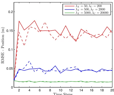
The first experiment illustrates the performance of the algorithms for different values of the mean total number of measurements in Fig. 1. The ratio between the mean number of clutter measurements and mean number of target measurements is fixed at 4:1. The RMSEs of the algorithms are in agreement, however, it is noted that an increase in the total mean number of measurements results in substantial com-putational savings. The amount of comcom-putational saving is as high as 80% with no significant loss in tracking performance. In Fig. 2 the ratio between the mean number of clutter mea-surements and mean number of target meamea-surements is varied. This allows for the observation of the performance when there is a varied amount of information about the target present in the measurements. The RMSE results show agreement between the two algorithms with an increase in computational savings when the mean number of target measurements is higher.
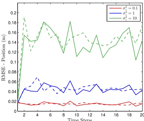
Fig. 3 illustrates the influence of varying the covariance matrix of the target observation model. The RMSEs of the two algorithms are in agreement. It is noted that a smaller computational saving is incurred as the measurement model becomes more precise. This result seems counter-intuitive. The reason for this is due to the Taylor approximation for the proxy. The upper bound for the range,RB
k, becomes a weaker bound
as the observation model becomes more peaked.
2 4 6 8 10 12 14 16 18 20 0
0.05 0.1 0.15 0.2
Time Steps
R
M
S
E
-P
o
si
ti
o
n
(m
)
λX= 50,λC= 200 λX= 500,λC= 2000 λX= 5000,λC= 20000
(a) RMSE comparison for different values of mean number of total measurements. The dotted lines represent the results from the standard sequential MCMC, and the full lines represent the results from the adaptive subsampling sequential MCMC.
0.2 0.3 0.4 0.5 0.6 0.7 0.8 0.9 1
λX= 50 λX = 500 λX= 5000 λC = 200 λC= 2000 λC= 20000
N
o
rm
a
li
ze
d
N
u
m
b
er
o
f
S
u
b
sa
m
p
le
d
M
ea
su
re
m
en
ts
[image:7.612.319.557.58.257.2](b) Comparison of the normalized number of subsampled measure-ments evaluated in the adaptive subsampling sequential MCMC for different values of mean number of total measurements.
Fig. 1: Performance comparison for a different mean number of total measurements with a constant clutter to target measurement ratio of 4:1.
V. CONCLUSION
In this paper, we presented an adaptive subsampling sequen-tial MCMC algorithm for target tracking. We have shown that this approach results in substantial computational savings when there is a large number of measurements, and most importantly, without sacrificing tracking performance.
2 4 6 8 10 12 14 16 18 20 0
0.02 0.04 0.06 0.08 0.1 0.12 0.14 0.16
Time Steps
R
M
S
E
-P
o
si
ti
o
n
(m
)
λX= 100
λX= 500
λX= 1000
(a) RMSE comparison of different values of mean target measure-ments. The dotted lines represent the results from the standard sequential MCMC, and the full lines represent the results from the adaptive subsampling sequential MCMC.
0.55 0.6 0.65 0.7 0.75 0.8 0.85 0.9 0.95 1
λX = 100 λX = 500 λX = 1000
N
o
rm
a
li
ze
d
N
u
m
b
er
o
f
S
u
b
sa
m
p
le
d
M
ea
su
re
m
en
ts
[image:8.612.319.556.58.257.2](b) Comparison of the normalized number of subsampled measure-ments evaluated in the adaptive subsampling sequential MCMC for different values of mean target measurements.
Fig. 2: Performance comparison for a different number of mean clutter to target measurements ratios.
ACKNOWLEDGMENTS
We would like to thank R´emi Bardenet for the constructive discussions on this work. We also acknowledge the support from the UK Engineering and Physical Sciences Research Council (EPSRC) via the Bayesian Tracking and Reasoning over Time (BTaRoT) grant EP/K021516/1 and EC Seventh Framework Programme [FP7 2013-2017] TRAcking in com-pleX sensor systems (TRAX) Grant agreement no.: 607400.
REFERENCES
[1] L. Mihaylova, A. Carmi, F. Septier, A. Gning, S. Pang, and S. Godsill, “Overview of Bayesian sequential Monte Carlo methods for group and
2 4 6 8 10 12 14 16 18 20
0 0.02 0.04 0.06 0.08 0.1 0.12 0.14 0.16 0.18 0.2
Time Steps
R
M
S
E
-P
o
si
ti
o
n
(m
)
σ2z= 0.1 σ2z= 1 σ2z= 10
(a) RMSE comparison for different measurement covariance matrices. The dotted lines represent the results from the standard sequential MCMC, and the full lines represent the results from the adaptive subsampling sequential MCMC.
0.75 0.8 0.85 0.9
N
o
rm
a
li
ze
d
N
u
m
b
er
o
f
S
u
b
sa
m
p
le
d
M
ea
su
re
m
en
ts
σ2
z= 0.1 σ
2
z= 1 σ
[image:8.612.57.294.59.257.2]2 z= 10 (b) Comparison of the normalized number of subsampled measure-ments evaluated in the adaptive subsampling sequential MCMC for different covariance matrices.
Fig. 3: Performance comparison for different covariance matrices whereΣ=σ2
zI.
extended object tracking,” Digital Signal Processing: A Review Journal, vol. 25, no. 1, pp. 1–16, 2014.
[2] S. Balakrishnan and D. Madigan, “A one-pass sequential Monte Carlo method for Bayesian analysis of massive datasets,” Bayesian Anal., vol. 1, no. 2, pp. 345–361, June 2006.
[3] N. Gordon, D. Salmond, and A. Smith, “Novel approach to nonlinear/non-Gaussian Bayesian state estimation,” IEE Proc. F Radar
and Signal Proc., vol. 140, no. 2, pp. 107–113, April 1993.
[4] W. R. Gilks and C. Berzuini, “Following a moving target-Monte Carlo inference for dynamic Bayesian models,” J. Royal Statist. Soc.: Series
B, vol. 63, no. 1, pp. 127–146, 2001.
[5] P. Djuric and M. Bugallo, “Particle filtering for high-dimensional systems,” in Proc. of the 5th IEEE Int. Workshop on Computational
Advances in Multi-Sensor Adaptive Processing, Dec. 2013, pp. 352–355.
279, 2007.
[7] Z. Khan, T. Balch, and F. Dellaert, “MCMC-based particle filtering for tracking a variable number of interacting targets,” IEEE Trans. on Pattern
Analysis and Machine Intelligence, vol. 27, no. 11, pp. 1805 –1819, Nov.
2005.
[8] F. Septier, S. K. Pang, A. Carmi, and S. Godsill, “On MCMC-Based particle methods for Bayesian filtering: Application to multitarget track-ing,” in Proc. of the IEEE Int. Workshop on Computational Advances in
Multi-Sensor Adaptive Processing, Dec. 2009, pp. 360–363.
[9] A. Korattikara, Y. Chen, and M. Welling, “Austerity in MCMC land: Cutting the Metropolis-Hastings Budget,” in Proc. of the Int. Conf. on
Machine Learning, 2014.
[10] R. Bardenet, A. Doucet, and C. Holmes, “Towards scaling up Markov chain Monte Carlo: an adaptive subsampling approach,” in Proc. of the
Int. Conf. on Machine Learning, 2014, pp. 405–413.
[11] ——, “Markov chain Monte Carlo and tall data,” preprint, http://arxiv.org/abs/1505.02827, May 2015.
[12] J.-Y. Audibert, R. Munos, and C. Szepesv´ari, “Exploration-exploitation tradeoff using variance estimates in multi-armed bandits,” Theoretical
Computer Science, vol. 410, no. 19, pp. 1876 – 1902, 2009.
[13] R. Bardenet and O.-A. Maillard, “Concentration inequalities for sampling without replacement,” To appear in Bernoulli, 2015. [Online]. Available: arxiv.org/abs/1309.4029