Generating custom propagators for arbitrary constraints

White Rose Research Online URL for this paper:

http://eprints.whiterose.ac.uk/144140/

Version: Published Version

Article:

Gent, Ian, Jefferson, Christopher, Linton, Steve et al. (2 more authors) (2014) Generating

custom propagators for arbitrary constraints. Artificial Intelligence. pp. 1-33. ISSN

0004-3702

https://doi.org/10.1016/j.artint.2014.03.001

[email protected]

https://eprints.whiterose.ac.uk/

Reuse

This article is distributed under the terms of the Creative Commons Attribution (CC BY) licence. This licence

allows you to distribute, remix, tweak, and build upon the work, even commercially, as long as you credit the

authors for the original work. More information and the full terms of the licence here:

https://creativecommons.org/licenses/

Takedown

If you consider content in White Rose Research Online to be in breach of UK law, please notify us by

Contents lists available atScienceDirect

Artificial Intelligence

www.elsevier.com/locate/artint

Generating custom propagators for arbitrary constraints

Ian P. Gent, Christopher Jefferson

∗

, Steve Linton, Ian Miguel, Peter Nightingale

∗

School of Computer Science, University of St Andrews, St Andrews, Fife KY16 9SX, UK

a r t i c l e

i n f o

a b s t r a c t

Article history:

Received 29 November 2012

Received in revised form 27 February 2014 Accepted 2 March 2014

Available online 12 March 2014

Keywords:

Constraint programming Constraint satisfaction problem Propagation algorithms Combinatorial search

Constraint Programming (CP) is a proven set of techniques for solving complex combinatorial problems from a range of disciplines. The problem is specified as a set of decision variables (with finite domains) and constraints linking the variables. Local reasoning (propagation) on the constraints is central to CP. Many constraints have efficient constraint-specific propagation algorithms. In this work, we generate custom propagators for constraints. These custom propagators can be very efficient, even approaching (and in some cases exceeding) the efficiency of hand-optimised propagators.

Given an arbitrary constraint, we show how to generate a custom propagator that establishes GAC in small polynomial time. This is done by precomputing the propagation that would be performed on every relevant subdomain. The number of relevant sub-domains, and therefore the size of the generated propagator, is potentially exponential in the number and domain size of the constrained variables.

The limiting factor of our approach is the size of the generated propagators. We investigate symmetry as a means of reducing that size. We exploit the symmetries of the constraint to merge symmetric parts of the generated propagator. This extends the reach of our approach to somewhat larger constraints, with a small run-time penalty.

Our experimental results show that, compared with optimised implementations of the table constraint, our techniques can lead to an order of magnitude speedup. Propagation is so fast that the generated propagators compare well with hand-written carefully optimised propagators for the same constraints, and the time taken to generate a propagator is more than repaid.

2014 The Authors. Published by Elsevier B.V. This is an open access article under the CC BY license (http://creativecommons.org/licenses/by/3.0/).

1. Introduction

Constraint Programming is a proven technology for solving complex combinatorial problems from a range of disciplines, including scheduling (nurse rostering, resource allocation for data centres), planning (contingency planning for air traffic control, route finding for international container shipping, assigning service professionals to tasks) and design (of crypto-graphic S-boxes, carpet cutting to minimise waste). Constraint solving of a combinatorial problem proceeds in two phases. First, the problem is modelled as a set of decision variables with a set of constraints on those variables that a solution must satisfy. A decision variable represents a choice that must be made in order to solve the problem. Consider Sudoku as a sim-ple examsim-ple. Each cell in the 9

×

9 square must be filled in such a way that each row, column and 3

×

3 sub-square contain all distinct non-zero digits. In a constraint model of Sudoku, each cell is a decision variable with the domain

{

1

. . .

9

}

. The

*

Corresponding authors.

E-mail addresses:[email protected](I.P. Gent),[email protected](C. Jefferson),[email protected](S. Linton),[email protected] (I. Miguel),[email protected](P. Nightingale).

http://dx.doi.org/10.1016/j.artint.2014.03.001

constraints require that subsets of the decision variables corresponding to the rows, columns and sub-squares of the Sudoku grid are assigned distinct values.

The second phase is solving the modelled problem using a constraint solver. A solution is an assignment to decision vari-ables satisfying all constraints, e.g. a valid solution to a Sudoku puzzle. A constraint solver typically works by performing a systematic search through a space of possible solutions. This space is usually vast, so search is combined with constraint

propagation, a form of inference that allows the solver to narrow down the search space considerably. A constraint prop-agator is an algorithm that captures a particular pattern of such inference, for example requiring each of a collection of variables to take distinct values. A state-of-the-art constraint solver has a suite of such propagators to apply as appropriate to an input problem. In this paper we will consider propagators that establish a property called Generalised Arc Consistency (GAC)[1], which requires that every value in the domains of the variables in the scope of a particular constraint participates in at least one assignment that satisfies that constraint.

Constraint models of structured problems often contain many copies of a constraint, which differ only in their scope. English Peg Solitaire,1 for example, is naturally modelled with amove constraint for each of 76 moves, at each of 31 time steps, giving 2356 copies of the constraint[2]. Efficient implementation of such a constraint is vital to solving efficiency, but choosing an implementation is often difficult.

The solver may provide a hand-optimised propagator matching the constraint. If it does not, the modeller can use a variety of algorithms which achieve GAC propagation for arbitrary constraints, for example GAC2001 [3], GAC-Schema [4], MDDC [5], STR2[6], the Trie table constraint[7], or Regular [8]. Typically these propagators behave well when the data structure they use (whether it is a trie, multi-valued decision diagram (MDD), finite automaton, or list of tuples) is small. They all run in exponential time in the worst case, but run in polynomial time when the data structure is of polynomial size.

The algorithms we give herein generate GAC propagators for arbitrary constraints that run in timeO

(

nd

)

(wherenis the number of variables anddis the maximum domain size), in extreme cases an exponential factor faster than any table con-straint propagator[3,7,9,5,6,10–13]. As our experiments show, generated propagators can even outperform hand-optimised propagators when performing the same propagation. It can take substantial time to generate a GAC propagator, however the generation time is more than repaid on the most difficult problem instances in our experiments.

Our approach is general but in practice does not scale to large constraints as it precomputes domain deletions for all possible inputs of the propagator (i.e. all reachable subsets of the initial domains). However, it remains widely applicable — like the aforementioned Peg Solitaire model, many other constraint models contain a large number of copies of one or more small constraints.

Propagator trees

Our first approach is to generate a binary tree to store domain deletions for all reachable subdomains. The tree branches on whether a particular literal (variable, value pair) is in domain or not, and each node of the tree is labelled with a set of domain deletions. After some background in Section2, the basic approach is described in Section3.

We have two methods of executing the propagator trees. The first is to transform the tree into a program, compile it and link it to the constraint solver. The second is a simple virtual machine: the propagator tree is encoded as a sequence of instructions, and the constraint solver has a generic propagator that executes it. Both these methods are described in Section3.5.

The generated trees can be very large, but this approach is made feasible for small constraints (both to generate the tree, and to transform, compile and execute it) by refinements and heuristics described in Section4. The binary tree approach is experimentally evaluated in Section5, demonstrating a clear speed-up on three different problem classes.

Exploiting symmetry

The second part of the paper is about exploiting symmetry. We define the symmetry of a constraint as a permutation group on the literals, such that any permutation in the group maintains the semantics of the constraint. This allows us to compress the propagator trees: any two subtrees that are symmetric are compressed into one. In some cases this replaces an exponential sized tree with a polynomially sized symmetry-reduced tree. Section6gives the necessary theoretical back-ground. In that section we develop a novel algorithm for finding the canonical image of a sequence of sets under a group that acts pointwise on the sets. We believe this is a small contribution to computational group theory.

Section 7describes how the symmetry-reduced trees are generated, and gives some bounds on their size under some symmetry groups. Executing the symmetry-reduced trees is not as simple as for the standard trees. Both the code generation and VM approaches are adapted in Section7.3.

In Section 8 we evaluate symmetry-reduced trees compared to standard propagator trees. We show that exploiting symmetry allows propagator trees to scale to larger constraints.

2. Theoretical background

We briefly give the most relevant definitions, and refer the reader elsewhere for more detailed discussion[1].

Definition 1. ACSP instance, P, is a triple

V

,

D

,

C

, where: V is a finite set ofvariables; D is a function from variables to theirdomains, where

∀

v

∈

V

:

D

(

v

)

⊂

Z

and D

(

v

)

is finite; and C is a set ofconstraints. A literalof P is a pair

v

,

d

, where v

∈

V andd

∈

D

(

v

)

. Anassignmentto any subset X

⊆

V is a set consisting of exactly one literal for each variable in X. Each constraint c is defined over a list of variables, denoted scope

(

c

)

. A constraint either forbids or allows each assignment to the variables in its scope. An assignment S toV satisfiesa constraintcif Scontains an assignment allowed byc. Asolutionto P is any assignment to V that satisfies all the constraints of P.

Constraint propagators work with subdomain lists, as defined below.

Definition 2. For a set of variables X

= {

x1

. . .

xn

}

with original domains D

(

x1

), . . . ,

D

(

xn

)

, asubdomain list S for X is a function from variables to sets of domain values that satisfies:

∀

i

∈ {

1

. . .

n

}

: S

(

xi

)

⊆

D

(

xi

)

. We extend the

⊆

notation to write R

⊆

S for subdomain lists Rand S iff

∀

i

∈ {

1

. . .

n

}

: R

(

xi

)

⊆

S

(

xi

)

. Given a CSP instance P

=

V

,

D

,

C

, asearch state forP is a subdomain list forV. An assignment A is contained in a subdomain listSiff

∀

v

,

d

∈

A: d

∈

S

(

v

)

(and ifS

(

v

)

is not defined thend

∈

S

(

v

)

is false).

Backtracking search operates on search states to solve CSPs. During solving, the search state is changed in two ways: branching and propagation. Propagation removes literals from the current search state without removing solutions. Herein, we consider only propagators that establish Generalised Arc Consistency (GAC), which we define below. Branching is the operation that creates a search tree. For a particular search state S, branching splits S into two statesS1 and S2, typically by splitting the domain of a variable into two disjoint sets. For example, in S1 branching might make an assignmentx

→

a (by excluding all other literals ofx), and inS2 remove only the literalx

→

a.S1 andS2are recursively solved in turn.

Definition 3.Given a constraintcand a subdomain list S ofscope

(

c

)

, a literal

v

,

d

issupportediff there exists an assign-ment that satisfiesc and is contained in S and contains

v

,

d

. SisGeneralised Arc Consistent (GAC)with respect toc iff, for everyd

∈

S

(

v

)

, the literal

v

,

d

is supported.

Any literal that does not satisfy the test inDefinition 3may be removed. In practice, CP solvers fail and backtrack if any domain is empty. Therefore propagators can assume that every domain has at least one value in it when they are called. Therefore we give a definition of GAC propagator that has as a precondition that all domains contain at least one value. This precondition allows us to generate smaller and more efficient propagators in some cases.

Definition 4. Given a CSP P

=

V

,

D

,

C

, a search state S for P where each variable x

∈

V has a non-empty domain:

|

S

(

x

)

|

>

0, and a constraintc

∈

C, theGAC propagatorforc returns a new search stateS′_which:

1. For all variables not inscope

(

c

)

: is identical to S.

2. For all variables inscope

(

c

)

: omits all (and only) literals inS that are not supported inc, and is otherwise identical to

S.

3. Propagator generation

We introduce this section by giving a naïve method that illustrates our overall approach. Then we present a more sophisticated method that forms the basis for the rest of this paper.

3.1. A naïve method

GAC propagation is NP-hard for some families of constraints defined intensionally. For example, establishing GAC on the constraint

ixi

=

0 is NP-hard, as it is equivalent to the subset-sum problem [14] (§35.5). However, given a constraint c onnvariables, each with domain sized, it is possible to generate a GAC propagator that runs in time O

(

nd

)

. The approach is to precompute the deletions performed by a GAC algorithm for every subdomain list for scope

(

c

)

. Thus, much of the computational cost is moved from the propagator (where it may be incurred many times during search) to the preprocessing step (which only occurs once).

The precomputed deletions are stored in an arrayT mapping subdomain lists to sets of literals. The generated propagator reads the domains (in O

(

nd

)

time), looks up the appropriate subdomain list in T and performs the required deletions. T

[image:5.561.143.409.57.206.2]

Fig. 1.Example of propagator tree for constraintx∨ywith initial domains of{0,1}.

T can be generated in O

((

2d

−

1

)

n

.

n

.

dn

)

time. There are 2d

−

1 non-empty subdomains of a size d domain, and so

(

2d

₋

₁

₎

n _{non-empty subdomain lists onnvariables. For each, GAC is enforced in O}

₍

_n

_.

_dn

₎

_{time and the set of deletions is} recorded. As there are at mostnddeletions,T is size at most

(

2d

₋

₁

₎

n

_.

_nd.

3.2. Propagator trees

The main disadvantage of the naïve method is that it computes and stores deletions for many subdomain lists that cannot be reached during search. A second disadvantage is that it must read the entire search state (for variables in scope) before looking up the deletions. We address both problems by using a tree to represent the generated propagator. The tree represents only the subdomain lists that arereachable: no larger subdomain list fails or is entailed. This improves the average- but not the worst-case complexity.

In this section we introduce the concept of a propagator tree. This is a rooted binary tree with labels on each node representing actions such as querying domains and pruning domain values. A propagator tree can straightforwardly be translated into a program or an executable bytecode. We will describe an algorithm that generates a propagator tree, given any propagator and entailment checker for the constraint in question. First we define propagator tree.

Definition 5. Apropagator tree nodeis a tuple T

=

Left

,

Right

,

Prune

,

Test

, whereLeftandRightare propagator tree nodes (orNil),Pruneis a set of literals to be deleted at this node, andTestis a single literal. Any of the items in the tuple may be

Nil. Apropagator treeis a rooted tree of nodes of typeT. The root node is namedr. We use dot to access members of a tree node v, so for example the left subtree is v

.

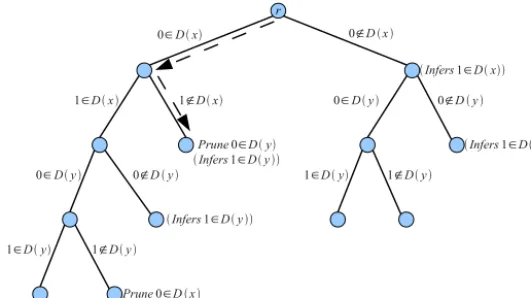
Left.

Example 1.Suppose we have the constraint x

∨

y with initial domains of

{

0

,

1

}

. An example propagator tree for this con-straint is shown in Fig. 1. The tree first branches to test whether 0

∈

D

(

x

)

. In the branch where 0

∈

/

D

(

x

)

, it infers that 1

∈

D

(

x

)

because otherwiseD

(

x

)

would be empty. Both subtrees continue to branch until the domains D

(

x

)

andD

(

y

)

are completely known. In two cases, pruning is required (when D

(

x

)

= {

0

}

and whenD

(

y

)

= {

0

}

).

An execution of a propagator tree follows a path in the tree starting at the root r. At each vertex v, the propagator prunes the set of literals specified by v

.

Prune. If v

.

Test is Nil, then the propagator is finished. Otherwise, the propagator tests if the literal v

.

Test

=

(

xi

,

a

)

is in the current subdomain list S. Ifa

∈

S

(

xi

)

, then the next vertex in the path is the left child v

.

Left, otherwise it is the right childv

.

Right. If the relevant child isNil, then the propagator is finished.

Example 2. Continuing fromExample 1, suppose we have D

(

x

)

= {

0

}

, D

(

y

)

= {

0

,

1

}

. The dashed arrows inFig. 1show the execution of the propagator tree, starting atr. First the value 0 of D

(

x

)

is tested, and found to be in the domain. Second, the value 1 ofD

(

x

)

is tested and found to be not in the domain. This leads to a leaf node where 0 is pruned fromD

(

y

)

. The other value of yis assumed to be in the domain (otherwise the domain is empty and the solver will fail and backtrack).

3.3. Comparing propagator trees to handwritten propagators

Handwritten propagators make use of many techniques for efficiency. For example they often have state variables that are incrementally updated and stored between calls to the propagator. They also make extensive use oftriggers— notifications from the solver about how domains have changed since the last call (for example, literal

x

,

a

has been pruned).

Algorithm 1SimpleGenTree(c,SD,ValsIn) 1: Deletions←Propagate(c,SD)

2:SD′_{←SD\Deletions}

3:ifall domains inSD′_{are emptythen}

4: return T= Prune=Deletions,Test=Nil,Left=Nil,Right=Nil

5:ValsIn∗←ValsIn\Deletions

6:ValsIn′←ValsIn∗∪ {(x,a)|(x,a)∈SD′_,|SD′_{(x)| =1}}

7:ifSD′_=ValsIn′

then

8: return T= Prune=Deletions,Test=Nil,Left=Nil,Right=Nil

{Pick a variable and value, and branch} 9:(y,l)←heuristic(SD′_\ValsIn′₎

10: LeftT←SimpleGenTree(c,SD′_,ValsIn′_∪(

y,l)) 11: RightT←SimpleGenTree(c,SD′_{\ {(y,l)},ValsIn}′

)

12:return T= Prune=Deletions,Test=(y,l),Left=LeftT,Right=RightT

we plan to create multiple propagator trees which will be executed for different trigger events, dividing responsibility for achieving GAC among the trees.

3.4. Generating propagator trees

SimpleGenTree (Algorithm 1) is our simplest algorithm to create a propagator tree given a constraintc and the initial domains D. The algorithm is recursive and builds the tree in depth-first left-first order. When constructed, each node in a propagator tree will test values to obtain more information about S, the current subdomain list (Definition 2). At a given tree node, each literal from the initial domains D may be in S, or out, or unknown (not yet tested). SimpleGenTree has a subdomain list SD for each tree node, representing values that are in S or unknown. It also has a second subdomain listValsIn, representing values that are known to be in S.Algorithm 1is called as SimpleGenTree(c, D,

∅

), wherec is the parameter of the Propagate function (called on line1) andD is the initial domains. For all our experiments, Propagate is a positive GAC table propagator and thuscis a list of satisfying tuples.

SimpleGenTree proceeds in two stages. First, it runs a propagation algorithm on SDto compute the prunings required given current knowledge of S. This set of prunings is conservative in the sense that they can be performed whatever the true value of Sbecause S

⊆

SD. The prunings are stored in the current tree node, and each pruned value is removed from

SD to form SD′. If a domain is empty in SD′, the algorithm returns. Pruned values are also removed from ValsInto form

ValsIn′ — these values are known to be in S, but the propagator tree will remove them from S. Furthermore, if only one value remains for some variable inSD′_{, the value is added toValsIn}′ _{(otherwise the domain would be empty).}

Propagate is assumed to empty all variable domains if the constraint is not satisfiable with the subdomain list SD. A GAC propagator (according toDefinition 4) will do this, however Propagate does not necessarily enforce GAC. The proof of correctness below is simplified by assuming Propagate always enforces GAC.

Throughout this paper we will only consider GAC propagators according toDefinition 4. If the Propagate function does not enforce GAC then the propagator tree that is generated does not necessarily enforce the same degree of consistency as Propagate. Characterising non-GAC propagator trees is not straightforward and we leave an investigation of this to future work.

The second stage is to choose a literal and branch. This literal is unknown, i.e. inSD′ _{but notValsIn}′_{. SimpleGenTree}

recurses for both left and right branches. On the left branch, the chosen literal is added toValsIn, because it is known to be present inS. On the right, the chosen literal is removed fromSD. There are two conditions that terminate the recursion. In both cases the algorithm attaches the deletions to the current node and returns. The first condition is that all domains have been emptied by propagation. The second condition isSD′

₌

_ValsIn′_{. At this point, we have complete knowledge of the}

current search state S:SD′

=

ValsIn′

=

S.

3.5. Executing a propagator tree

We compare two approaches to executing propagator trees. The first is to translate the tree into program code and compile it into the solver. This results in a very fast propagator but places limitations on the size of the tree. The second approach is to encode the propagator tree into a stream of instructions, and execute them using a simple virtual machine.

3.5.1. Code generation

Algorithm 2(GenCode) generates a program from a propagator tree via a depth-first, left-first tree traversal. It is called initially with the rootr. GenCode creates the body of the propagator function, the remainder is solver specific. In the case of Minion solver specific code is very short and the same for all propagator trees.

3.5.2. Virtual machine

Algorithm 2GenCode(Propagator treeT, vertexv) 1:ifv=Nilthen

2: WriteToCode(“NoOperation;") 3:else

4: WriteToCode(“RemoveValuesFromDomains("+v.Prune+“);") 5: ifv.Test=Nilthen

6: (xi,a)←v.Test

7: WriteToCode(“if IsInDomain("+a+“,"+xi+“) then")

8: GenCode(T,v.Left) 9: WriteToCode(“else") 10: GenCode(T,v.Right) 11: WriteToCode(“endif;")

Branch :

var

,

val

,

pos

— If the value valisnot in the domain of the variable var then jump to position pos. Otherwise, execution continues with the next instruction in the sequence. A jump to

−

1 ends execution of the virtual machine. Prune :

var1

,

val1

,

var2

,

val2

, . . . ,

−

1

— Prune a set of literals from the variable domains. The operands are a list of

variable–value pairs terminated by

−

1.

Return : — End execution of the virtual machine.

Tree nodes are encoded in depth-first left-first order, and execution of the instruction stream starts at location 0. Any node that has a left child is immediately followed by its left child. The Branch instruction will either continue at the next instruction (the left child) or jump to the location of the right child. When an internal node is encoded, the position of its right child is not yet known. We insert placeholders forposin the branch instruction and fill them in during a second pass. The VM clearly has the advantage that no compilation is required, however it is somewhat slower than the code gener-ation approach in our experiments below.

3.6. Correctness

In order to prove the SimpleGenTree algorithm correct, we assume that the Propagate function called on line1enforces GAC exactly as in Definition 3. In particular, if Propagate produces a domain wipe-out, it must delete all values of all variables in the scope. This is not necessarily the case for GAC propagators commonly used in solvers. We also assume that the target constraint solver removes all values of all variables in a constraint if our propagator tree empties any individual domain. In practice, constraint solvers often have some shortcut method, such as a special functionFailfor these situations, but our proofs are slightly cleaner for assuming domains are emptied. Finally we implicitly match up nodes in the generated trees with corresponding points in the generated code for the propagator. Given these assumptions, we will prove that the code we generate does indeed establish GAC.

Lemma 1.Assuming that the Propagate function in line1establishes GAC, then: given inputs

(

c

,

SD

,

ValsIn

)

, ifAlgorithm 1returns at line4or line8, the resulting set of prunings achieve GAC for the constraint c on any search state S such that ValsIn

⊆

S

⊆

SD.

Proof. IfAlgorithm 1returns on either line4or line8, the set of deletions returned are those generated on line1. These deletions achieve GAC propagation for the search stateSD.

If the GAC propagator forc would remove a literal fromSD, then that literal is in no assignment which satisfiesc and is contained in SD. As S is contained in SD, that literal must also be in no assignment that satisfiesc and is contained in S. Therefore any literals inS that are removed by a GAC propagator forSDwould also be removed by a GAC propagator for S. We now show no extra literals would be removed by a GAC propagator for S. This is separated into two cases. The first case is if Algorithm 1returns on line4. Then GAC propagation onSD has removed all values from all domains. There are therefore no further values which can be removed, so the result follows trivially.

The second case is if Algorithm 1returns on line8. ThenSD′

=

ValsIn′on line7. Any literals added toValsIn′on line6

are also in S, as literals are added when exactly one value exists in the domain of a variable in SD, and so this value must also be inS, otherwise there would be an empty domain in S. Thus we haveValsIn′

⊆

(

S

\

Deletions

)

⊆

SD′_{. But since}

ValsIn′

=

SD′, we also have SD′

=

S

\

Deletions. Since we knowSD′ is GAC by the assumed correctness of the Propagate function, so is S

\

Deletions.

2

Theorem 1.Assuming that the Propagate function in line1establishes GAC, then: given inputs

(

c

,

SD

,

ValsIn

)

, then the code generator

Algorithm 2applied to the result ofAlgorithm 1returns a correct GAC propagator for search states S such that ValsIn

⊆

S

⊆

SD.

By the same argument used inLemma 1, the Deletions generated on line1can also be removed from S. If applying these deletions to S leads to a domain wipe-out, then the constraint solver sets S

(

x

)

= ∅

for allx

∈

scope

(

c

)

, and the propagator has established GAC, no matter what happens in the rest of the tree.

If no domain wipe-out occurs, we progress to line9. At this point we know thatValsIn′

⊆

S

\

Deletions

⊆

SD′. Also, since we passed line7, we know thatValsIn′

=

SD′_{, and therefore there is at least one literal for the heuristic to choose. There are}

now two cases. The literal

(

y

,

l

)

chosen by the heuristic is in S, or not.

Ifl

∈

S

(

y

)

, then the generated propagator will branch left. The propagator generated after this branch is generated from the tree produced by SimpleGenTree

(

c

,

SD′

_,

_ValsIn′

_∪

(

y

,

l

))

. Sincel

∈

S

(

y

)

, we haveValsIn′

∪

(

y

,

l

)

⊆

S

\

Deletions

⊆

SD′_{. Since}

the tree on the left is strictly smaller, we can appeal to the induction hypothesis that we have generated a correct GAC propagator forS

\

Deletions. Since we know that Deletions were correctly deleted fromS, we have a correct GAC propagator at this node forS.

Ifl

∈

/

S

(

y

)

, the generated propagator branches right. The propagator on the right is generated from the tree given by SimpleGenTree

(

c

,

SD′

_\

₍

_y

_,

_l

_),

_ValsIn′

)

on S

\

Deletions. Here we have ValsIn′

⊆

S

\

Deletions

⊆

SD′

_\

₍

_y

_,

_l

₎

_{. As in the previous}

case, the requirements of the induction hypothesis are met and we have a correct GAC propagator for S.

Finally we note that the setSD

\

ValsInis always reduced by at least one literal on each recursive call to Algorithm 1. Therefore we know the algorithm will eventually terminate.

2

Corollary 1.Assuming the Propagate function correctly establishes GAC for any constraint c, then the code generatorAlgorithm 2

applied to the result ofAlgorithm 1with inputs

(

c

,

D

,

∅

)

, where D are the initial domains of the variables in c, generates a correct GAC propagator for all search states.

Lemma 2.If r is the time a solver needs to remove a value from a domain, and s the time to check whether or not a value is in the domain of a variable, the code generated byAlgorithm 2runs in time O

(

ndmax

(

r

,

s

))

.

Proof. The execution of the algorithm is to go through a single branch of an if/then/else tree. The tree cannot be of depth greater thannd since one literal is chosen at each depth and there are at most nd literals in total. Furthermore, on one branch any given literal can either be removed from a domain or checked, but not both. This is becauseAlgorithm 1never chooses a test from a removed value. Therefore the worst case isnd occurrences of whichever is more expensive out of testing domain membership and removing a value from a domain.

2

In some solvers bothr ands are O

(

1

)

, e.g. where domains are stored only in bitarrays. In such solvers our generated GAC propagator is O

(

nd

)

.

4. Generating smaller trees

Algorithm 3shows the GenTree algorithm. This is a refinement of SimpleGenTree. We present this without proof of cor-rectness, but a proof would be straightforward since the effect is only to remove nodes in the tree for which no propagation can occur in the node and the subtree beneath it.

The first efficiency measure is that GenTree always returnsNilwhen no pruning is performed at the current node and both children areNil, thus every leaf node of the generated propagator tree performs some pruning. The second measure is to use an entailment checker. A constraint isentailed with respect to a subdomain listSDif every tuple allowed onSD

is allowed by the constraint. When a constraint is entailed there is no possibility of further pruning. We assume we have a function entailed

(

c

,

SD

)

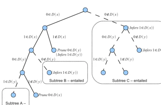
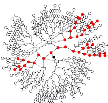
to check this. The function is called at the start of GenTree, and also after the subdomain list is updated by pruning (line9). In both cases, entailment leads to the function returning before making the recursive calls.

To illustrate the difference between SimpleGenTree and GenTree, considerFig. 2. The constraint is very small (x

∨

y on boolean variables, the same constraint as used inFig. 1) but even so SimpleGenTree generates 7 more nodes than GenTree. The figure illustrates the effectiveness and limitations of entailment checking. Subtree C contains no prunings, therefore it would be removed by GenTree with or without entailment checking. However, the entailment check is performed at the topmost node in subtree C, and GenTree immediately returns (line2) without exploring the four nodes beneath. Subtree B is entailed, but the entailment check does not reduce the number of nodes explored by GenTree compared to SimpleGenTree. Subtree A is not entailed, however GAC does no prunings here so GenTree will explore this subtree but not output it.

4.1. Bounds on tree size

At each internal node, the tree branches for some literal inSD′_{that is not inValsIn}′_{. Each unique literal may be branched}

on at most once down any path from the root to a leaf node. This means the number of bifurcations is at mostnd down any path. Therefore the size of the tree is at most 2

×

(

2nd

₎

₋

₁

₌

₂nd+1

₋

_{1 which isO}

₍

₂nd

₎

_.

Algorithm 3Generate propagator tree: GenTree(c,SD,ValsIn) 1:ifentailed(c,SD)then

2: return Nil

3: Deletions←Propagate(c,SD) 4:SD′_{=SD\Deletions}

5:ifall domains inSD′_{are emptythen}

6: return T= Prune=Deletions,Test=Nil,Left=Nil,Right=Nil

7:ValsIn∗←ValsIn\Deletions

8:ValsIn′_←ValsIn∗_{∪ {(x,a)|(x,a)∈SD}′_,|SD′_{(x)| =1}}

9:ifSD′_=ValsIn′_{or entailed(c,SD}′_)then

10: ifDeletions= ∅then

11: return Nil 12: else

13: return T= Prune=Deletions,Test=Nil,Left=Nil,Right=Nil

{Pick a variable and value, and branch} 14: (y,l)←heuristic(SD′_\ValsIn′₎

15: LeftT←GenTree(c,SD′_,ValsIn′_∪(y,l))

16: RightT←GenTree(c,SD′_{\ {(y,l)},ValsIn}′₎

17:ifLeftT=NilAnd RightT=NilAnd Deletions= ∅then

18: return Nil 19: else

[image:9.561.141.408.262.437.2]

20: return T= Prune=Deletions,Test=(y,l),Left=LeftT,Right=RightT

Fig. 2.Example of propagator tree for constraintx∨ywith initial domains of{0,1}. The entire tree is generated by SimpleGenTree (Algorithm 1). The more sophisticated algorithm GenTree (Algorithm 3) does not generate the subtrees A, B and C.

For many constraints GenTree is very efficient and does not approach its upper bound. The lemma below gives an example of a constraint where GenTree does generate a tree of exponential size.

Lemma 3.Consider the parity constraint on a list of variables

x1

, . . . ,

xn

with domain

{

0

,

1

}

. The constraint is satisfied when the sum

of the variables is even. Any propagator tree for this constraint must have at least2n−1_nodes.

Proof. The parity constraint propagates in exactly one case. When all but one variable is assigned, the remaining variable must be assigned such that the parity constraint is true. If there are two or more unassigned variables, then no propagation can be performed.

Suppose we select the first n

−

1 variables and assign them in any way (naming the assignment A), leaving xn unas-signed. xn must then be assigned either 0 or 1 by pruning, and the value depends on every other variable (and on every other variable being known to be assigned). The tree node that performs the pruning for A cannot be reached for any other assignment B

=

A to the firstn

−

1 variables, as the node for A requires knowing the whole of A to be able to prunexn. Therefore there must be a distinct node in the propagator tree for each of the 2n−1assignments to the firstn

−

1 variables.

2

4.2. Heuristic

[image:10.561.36.505.87.223.2]

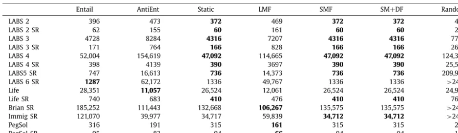
Table 1

Size of propagator tree for proposed heuristics and anti-heuristics. Figures for the Random heuristic are a mean of ten trees, each other tree was generated once. Where it took longer than 24 hours to generate a single tree, the entry reads>24 h. SR denotes symmetry-reduced trees.

Entail AntiEnt Static LMF SMF SM+DF Random

LABS 2 396 473 372 469 372 372 488

LABS 2 SR 62 155 60 161 60 60 265

LABS 3 4728 8284 4316 7207 4316 4316 7780

LABS 3 SR 171 764 166 828 166 166 2658

LABS 4 52,004 154,619 47,092 114,665 47,092 47,092 124,381

LABS 4 SR 398 4139 390 3697 390 390 25,550

LABS5 SR 747 16,613 736 14,373 736 736 209,970

LABS 6 SR 1287 62,172 1336 49,767 1336 1336 >24 h

Life 28,351 11,057 26,524 12,061 26,524 26,524 24,904

Life SR 740 683 410 476 410 410 7682

Brian SR 185,252 111,443 132,668 106,267 135,575 135,575 >24 h

Immig SR 121,070 39,977 34,717 59,839 34,712 34,712 >24 h

PegSol 316 191 315 161 315 315 222

PegSol SR 95 83 94 66 94 94 160

Entailment heuristic

To minimise the size of the tree, the aim of this heuristic is to cause Algorithm 3to return before branching. There are a number of conditions that cause this: entailment (lines 1 and 9); domain wipe-out (line 6); and complete domain information (line9).

The proposed heuristic greedily attempts to make the constraint entailed. This is done by selecting the literal contained in the greatest number of disallowed tuples ofc that are valid with respect toSD′. If this literal is invalid (as in the right subtree beneath the current node), then the greatest possible number of disallowed tuples will be removed from the set.

Smallest Domain heuristics

Smallest Domain First (SDF) is a popular variable ordering heuristic for CP search. We investigate two ways of adapting SDF. The first, Smallest Maybe First (SMF) selects a variable with the smallest non-zero number of literals inSD′

_\

_ValsIn′_.

SMF will tend to prefer variables with small initial domains, then prefer to obtain complete domain information for one variable before moving on to the next. Preferring small domains could be a good choice because on average each deleted value from a small domain will be in a large number of satisfying tuples. Ties are broken by the static order of the variables in the scope. Once a variable is chosen, the smallest literal for that variable is chosen fromSD′

_\

_ValsIn′_.

The second adaptation is Smallest Maybe

+

Domain First (SM

+

DF). This is similar to SMF with two changes: when se-lecting the variableSD′is used in place ofSD′

\

ValsIn′, and variables are chosen from the set of variables that have at least one literal inSD′

\

ValsIn′(otherwise SM

+

DF could choose a variable with no remaining literals to branch on).

Comparison

We compare the three proposed heuristics Entail, SMF and SM

+

DF against corresponding anti-heuristics AntiEntail and LMF (Largest Maybe First), one static ordering, and a dynamic random ordering (at each node a literal is chosen at random with uniform probability). We used all the constraints from both sets of experiments (in Sections5and8).

The static ordering for Peg Solitaire and LABS is the order the constraints are written in Sections5.2and5.3respectively. For Life, Immigration and Brian’s Brain, the neighbour variables are branched first, then the variable representing the current time-step, then the next time-step.

Table 1 shows the size of propagator trees for each of the heuristics. Static, SMF and SM

+

DF performed well overall. SMF and SM

+

DF produced trees of identical size. In two cases (Brian Sym and Immigration Sym) the tree generated with the static ordering is slightly larger than SMF. In most cases SMF performed better than its anti-heuristic LMF. SMF also has the advantage that the user need not provide an ordering.

Comparing the Entailment heuristic to Random shows that Entailment does have some value, but Entailment proved to be worse than SMF and Static in most cases. Also, Entailment is beaten by its anti-heuristic in 6 cases as opposed to 4 for SMF.

We use the SMF heuristic for all experiments in Sections5and8.

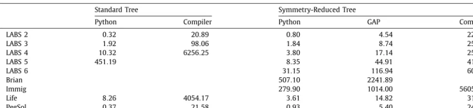
4.3. Implementation of GenTree

[image:11.561.153.397.78.120.2]

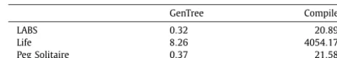
Table 2

Time taken to generate the propagator trees in Python and the C++compiler.

GenTree Compiler

LABS 0.32 20.89

Life 8.26 4054.17

Peg Solitaire 0.37 21.58

is entailed. It is also used to calculate the entailment heuristic described above. It is implemented in Python and is not highly optimised. It is executed using the PyPy JIT compiler2_{version 1.9.0.}

5. Experimental evaluation of propagator trees

In all the case studies below, we use the solver Minion [16]0.15. We experiment with 3 propagator trees, in each case comparing against hand-optimised propagators provided in Minion, and also against generic GAC propagators (as described in the subsection below). All instances were run 5 times and the mean was taken. In all cases times are given for an 8-core Intel Xeon E5520 at 2.27 GHz with 12 GB RAM. Minion was compiled with g

++

4.7.3, optimisation level

−

O3. For all experiments 6 Minion processes were executed in parallel. We ran all experiments with a 24 hour timeout, except where otherwise stated.

Table 2 reports the time taken to run GenTree, and separately to compile each propagator and link it to Minion. The propagator trees are compiled exactly as every other constraint in Minion is compiled. Specifically they are compiled once for each variable type, 7 times in total. In the case of Life, in our previous work[15]we compiled the propagator tree once (for Boolean variables), taking 217 s, whereas here it takes 4054.17 s. In each experiment in this section, we build exactly one propagator tree, which is then used for all instances in that experiment, and on multiple scopes for each instance.

5.1. Generic GAC propagators

In some cases a generic GAC propagator can enforce GAC in polynomial time. Typically this occurs if the size of the data structure representing the constraint is bounded by a polynomial. Generic propagators can also perform well when there is no polynomial time bound simply because they have been the focus of much research effort.

We compare propagator trees to three table constraints: Table, Lighttable, and STR2

+

. Table uses a trie data structure with watched literals[7]. Lighttable employs the same trie data structure but is stateless and uses static triggers. Lighttable searches for support for each value of every variable each time it is called. Finally STR2

+

is the optimised simple tabular reduction propagator by Lecoutre[6].

We also compare against MDDC, the MDD propagator of Cheng and Yap [5]. The MDD is constructed from the set of satisfying tuples. The MDDC propagator is implemented exactly as described by Cheng and Yap, and we used the sparse set variant. To construct the MDD, we used a simpler algorithm than Cheng and Yap. Our implementation first builds a complete trie representing the positive tuples, then converts the trie to an MDD by compressing identical subtrees.

Many of our benchmark constraints can be represented compactly using a Regular constraint [8]. We manually created deterministic finite automata for these constraints. These automata are given elsewhere[17]for space reasons. In the exper-iments we use the Regular decomposition of Beldiceanu et al.[18]which has a sequence of auxiliary variables representing the state of the automaton at each step, and a set of ternary table constraints each representing the transition table. We enforce GAC on the table constraints and this obtains GAC on the original Regular constraint.

5.2. Case study: English Peg Solitaire

English Peg Solitaire is a one-player game played with pegs on a board. It is Problem 37 atwww.csplib.org. The game and a model are described by Jefferson et al.[2]. The game has 33 board positions (fields), and begins with 32 pegs and one hole. The aim is to reduce the number of pegs to 1. At each move, a peg (A) is jumped over another peg (B) and into a hole, and B is removed. As each move removes one peg, we fix the number of time steps in our model to 32.

The model we use is as follows. The board is represented by a Boolean arrayb

[

32

,

33

]

where the first index is the time step

{

0

. . .

31

}

and the second index is the field

{

1

. . .

33

}

. The moves are represented by Boolean variables moves

[

31

,

76

]

, where the first index is the time step

{

0

. . .

30

}

(where move 0 connects board states 0 and 1), and the second index is the move number, where there are 76 possible moves. The third set of Boolean variables are equal

[

31

,

33

]

, where the first index is the time step

{

0

. . .

30

}

and the second is the field. The following constraint is posted for each equal variable:

equal

[

x

,

y

] ⇔

(

b

[

x

,

y

] =

b

[

x

+

1

,

y

]

)

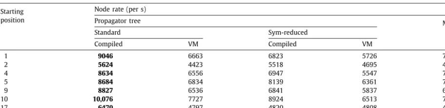
. The board state for the first and last time step are filled in, with one hole at the starting position, and one peg at the same position in the final time step. We consider only starting positions 1, 2, 4, 5, 9, 10, or 17, because all other positions can be reached by symmetry from one of these seven.

Table 3

Results on peg solitaire problems.

Starting position

Node rate (per s) _Nodes

Propagator tree Min Reified

Sumgeq

Compiled VM

1 9046 6663 7445 3953 –

2 5624 4423 4714 3329 10,268

4 8634 6556 7064 4007 –

5 8684 6834 7565 4318 –

9 8827 6536 6990 4114 –

10 10,076 7727 7921 4694 1,486,641

17 6470 4797 4702 3502 10,269

Starting position

Node rate (per s)

Lighttable Table MDDC Regular STR2+

1 755 1992 1902 326 1373

2 715 1657 1697 301 1281

4 672 2067 1597 304 1269

5 754 2206 1749 345 1385

9 735 1738 1682 297 1290

10 719 1931 1848 312 1437

17 701 1827 1686 303 1206

For each time step t

∈ {

0

. . .

30

}

, exactly one move must be made, therefore constraints are posted to enforce

imoves

[

t

,

i

] =

1. Also for each time stept, the number of pegs on the board is 32

−

t, therefore constraints are posted to enforce

33

i=1b

[

t

,

i

] =

32

−

t.

The bulk of the constraints model the moves. At each time stept

∈ {

0

. . .

30

}

, for each possible movem

∈ {

0

. . .

75

}

, the effects of movemare represented by an arity 7 Boolean constraint. Movemjumps a piece from field f1to f3over field f2. The constraint is as follows.

b

[

t,f1

] ∧ ¬

b

[

t

+

1,f1

] ∧

b

[

t,f2

] ∧ ¬

b

[

t

+

1,f2

] ∧ ¬

b

[

t,f3

] ∧

b

[

t

+

1,f3

]

⇔

moves

[

t

,m

]

Also, a frame constraint is posted to ensure that all fields other than f1, f2 and f3 remain the same. The constraint states (for all relevant fields f4) thatequal

[

t

,

f4

] =

1 whenmoves

[

t

,

m

] =

1.

In this experiment, the arity 7 move constraint is implemented in nine different ways, and all other constraints are invariant. First the move constraint is implemented as a propagator tree (compiled or using the VM). As shown inTable 2, the propagator tree was generated by GenTree in 0.37 s and compiled in 21.58 s. The tree has 315 nodes, and GenTree explored 509 nodes.

The Reified Sumgeq implementation uses a sum to represent the conjunction. The negation of some b variables is achieved with views [19], therefore no auxiliary variables are introduced. The sum constraint is reified to the moves

[

t

,

m

]

variable, as follows:

[

(

b

[

t

,

f1

] + · · · +

b

[

t

+

1

,

f3

]

)

6

] ⇔

moves

[

t

,

m

]

.

The Min implementation uses a single

min

constraint. Again views are used for negation and no auxiliary variables are introduced. The constraint is as follows:min

(

b

[

t

,

f1

]

, . . . ,

b

[

t

+

1

,

f3

]

)

=

moves

[

t

,

m

]

.

The move constraint is also implemented using the Lighttable, Table, MDDC and STR2

+

propagators. The table has 64 satisfying tuples. The Regular implementation [17] has 9 states and uses a ternary table constraint (representing the transition table) with 17 satisfying tuples.

Table 3shows our results for peg solitaire. All nine methods enforce GAC, therefore they search exactly the same space. When one or more methods completed the search within the 24 hour timeout, we give the node count. The compiled propagator tree outperforms Min by a substantial margin, which is perhaps remarkable given that Min is a hand-optimised propagator. The compiled propagator tree outperforms Reified Sumgeq by an even wider margin. None of the generic GAC methods Lighttable, Table, MDDC, Regular or STR2

+

come close to the handwritten propagators or the propagator tree. For the harder instances, the compiled propagator tree more than repays the overhead of its generation and compilation compared to Min. For example instance 10 was solved in 187 s by the Min implementation and 147 s (169 s when including the cost of building the propagator tree) with propagator trees.

5.3. Case study: low autocorrelation binary sequences

The Low Autocorrelation Binary Sequence (LABS) problem is described by Gent and Smith[20]. The problem is to find a sequencesof lengthnof symbols

{−

1

,

1

}

. For each intervalk

∈ {

1

. . .

n

−

1

}

, the correlationCkis the sum of the products

s

[

i

] ×

s

[

i

+

k

]

for alli

∈ {

0

. . .

n

−

k

−

1

}

. The overall correlation Cminis the sum of the squares of all Ck:Cmin

=

kn=−11

(

Ck

)

2.

Cminmust be minimised.

The sequence is modelled directly, using variabless

[

n

] ∈ {−

1

,

1

}

. For eachk

∈ {

1

. . .

n

−

1

}

, and each i

∈ {

0

. . .

n

−

k

−

1

}

, we have a variable pi

Table 4

Results on LABS problems of size 25–30. All times are a mean of 5 runs.

n Time (s)

Propagator tree Product Light-table

Table MDDC Reglr STR2+

Compiled VM

25 9.22 10.03 11.57 22.42 20.06 18.49 47.13 14.00

26 18.85 20.46 21.95 42.00 44.45 41.88 103.49 28.88

27 42.21 40.88 49.72 87.68 84.53 92.12 233.94 59.81

28 81.44 82.29 95.62 196.64 173.16 167.16 437.02 114.85 29 131.40 136.42 170.72 317.48 283.93 291.70 701.04 220.60 30 237.06 239.63 276.64 539.49 502.08 535.10 1199.77 348.53

n Search nodes Node rate (per s)

All GAC methods

Product Propagator tree Product

Compiled VM

25 206,010 350,119 22,344 20,541 30,260

26 404,879 709,228 21,481 19,788 32,309

27 790,497 1,343,545 18,726 19,335 27,022

28 1,574,100 2,684,883 19,328 19,129 28,077

29 2,553,956 4,441,023 19,437 18,722 26,014

30 4,120,335 7,118,749 17,381 17,194 25,733

variableCk

∈ {−

n

. . .

n

}

.Ckis constrained to be the sum of p_ki for alli. There are also variablesC_k2

∈ {

0

. . .

n2

}

, and a binary

lighttable

constraint is used to link Ck and C2k. Finally we have Cmin

=

kn−=11C2k, and Cmin is minimised. Gent and Smith identified 7 symmetric images of the sequence [20]. For each symmetric image we post one

lexleq

(lexicographic ordering) constraint to break the symmetry. Gent and Smith also proposed a variable and value ordering that we use here.

There are more ternary product constraints than any other constraint in LABS. Ck is a sum of products: Ck

=

(

s

[

0

] ×

s

[

k

]

)

+

(

s

[

1

] ×

s

[

k

+

1

]

)

+ · · ·

. To test propagator trees on this problem, we combine pairs of product constraints into a

single arity 5 constraint:

(

s

[

i

] ×

s

[

k

+

i

]

)

+

(

s

[

i

+

1

] ×

s

[

k

+

i

+

1

]

)

=

p_ki. This allows almost half of the p_ki variables to be removed. When there are an odd number of products, one of the original product constraints is retained for the largest value ofi.

We compare eight models of LABS:Product, the model with ternary product constraints;Propagator tree, where the new 5-ary constraint has a propagator tree, and this is either compiled or executed in the VM;Table,Lighttable,MDDCandSTR2

+

where the 5-ary constraint is implemented with a generic propagator using a table with 16 satisfying tuples; and Regular

[17]which has 10 states and uses a ternary table constraint (representing the transition table) with 17 satisfying tuples. All models exceptProductenforce GAC on the 5-ary constraint. All other constraints are the same for all eight models.

As shown inTable 2, the propagator tree was generated by GenTree in 0.32 s. The algorithm explored 621 nodes and the tree has 372 nodes. It was compiled in 20.89 s.

Table 4 shows our results for LABS sizes 25 to 30. The instances were solved to optimality. The Propagator Tree, Ta-ble, LighttaTa-ble, MDDC, Regular and STR2

+

models search the same number of nodes as each other, and exhibit stronger propagation than Product, but their node rate is lower than Product in all cases. The generic GAC propagator (and Regular decomposition) models are slower than Product. However, both propagator tree variants are faster than Product, and for the larger instances it more than repays the overhead of compiling the specialised constraint.

The virtual machine also performs better than might be expected, almost matching the speed of the compiled propagator tree while saving the compilation time.

5.4. Case study: maximum density oscillating life

Conway’s Game of Life was invented by John Horton Conway. The game is played on a square grid. Each cell in the grid is in one of two states (aliveordead). The state of the board evolves over time: for each cell, its new state is determined by its previous state and the previous state of its eight neighbours (including diagonal neighbours).Oscillatorsare patterns that return to their original state after a number of steps (referred to as theperiod). A period 1 oscillator is named astill life.

Various problems in Life have been modelled in constraints. Bosch and Trick considered period 2 oscillators and still lifes[21]. Smith[22]and Chu et al.[23]considered the maximum-density still life problem. Here we consider the problem of finding oscillators of various periods. We use simple models for the purpose of evaluating the propagator generation technique rather than competing with the sophisticated still-life models in the literature. However, to our knowledge we present the first model of oscillators of period greater than 2.

The problem of sizen

×

n (i.e. live cells are contained within ann

×

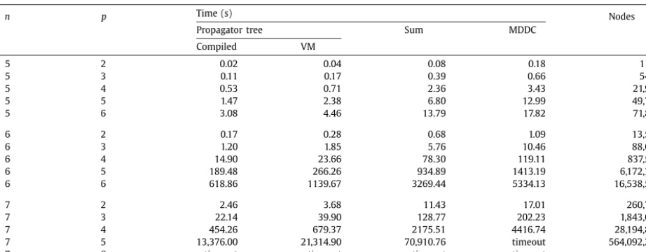
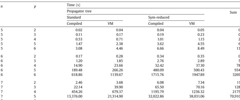
n bounding box at each time step) and period p

[image:14.561.41.502.78.258.2]

Table 5

Time to solve to optimality for propagator tree, sum and MDDC implementations of the Life constraint.

n p Time (s) Nodes

Propagator tree Sum MDDC

Compiled VM

5 2 0.02 0.04 0.08 0.18 1166

5 3 0.11 0.17 0.39 0.66 5489

5 4 0.53 0.71 2.36 3.43 21,906

5 5 1.47 2.38 6.80 12.99 49,704

5 6 3.08 4.46 13.79 17.82 71,809

6 2 0.17 0.28 0.68 1.09 13,564

6 3 1.20 1.85 5.76 10.46 88,655

6 4 14.90 23.66 78.30 119.11 837,541

6 5 189.48 266.26 934.89 1413.19 6,172,319

6 6 618.86 1139.67 3269.44 5334.13 16,538,570

7 2 2.46 3.68 11.43 17.01 260,787

7 3 22.14 39.90 128.77 202.23 1,843,049

7 4 454.26 679.37 2175.51 4416.74 28,194,835

7 5 13,376.00 21,314.90 70,910.76 timeout 564,092,290

7 6 timeout timeout timeout timeout –

andn

+

3 are set to 0. For a cellb

[

i

,

j

,

t

]

at time stept, the liveness of its successorb

[

i

,

j

, (

t

+

1

)

modp

]

is determined as follows. The 8 adjacent cells are summed:s

=

adjacent

(

b

[

i

,

j

,

t

]

)

, and the transition rules are as follows:

•

(

s

>

3

∨

s

<

2

)

⇒

b

[

i

,

j

, (

t

+

1

)

mod p

] =

0;

•

(

s

=

3

)

⇒

b

[

i

,

j

, (

t

+

1

)

modp

] =

1; and

•

(

s

=

2

)

⇒

b

[

i

,

j

, (

t

+

1

)

modp

] =

b

[

i

,

j

,

t

]

.

We refer to the grid at a particular time step as a layer. For each pair of layers, a

watchvecneq

(vector not-equal) constraint is used to constrain them to be distinct. To break some symmetries, the first layer is constrained to be lex less than all subsequent layers. Also, the first layer may be reflected horizontally and vertically, and rotated 90 degrees, so it is constrained to be lex less or equal than each of its 7 symmetric images. To find oscillators of maximum density, the number of dead cells in the first layer is summed to a variablemwhich is then minimised.

The liveness constraint involves 10 Boolean variables. As shown inTable 2, GenTree takes 8.26 s. The algorithm explored 86,685 nodes, and the resulting propagator tree has 26,524 nodes. Compilation took 4054.17 s.

The propagator tree is compared to six other implementations. The Sum implementation adds an auxiliary variable

s

[

i

,

j

,

t

] ∈

0

. . .

8 for each b

[

i

,

j

,

t

]

, and the sum constraint s

[

i

,

j

,

t

] =

adjacent

(

b

[

i

,

j

,

t

−

1

]

)

. s

[

i

,

j

,

t

]

, b

[

i

,

j

,

t

−

1

]

and

b

[

i

,

j

,

t

]

are linked by a ternary table (

lighttable

) constraint encoding the liveness rules. The Table, Lighttable,MDDC

and STR2

+

implementations simply encode the arity 10 constraint using a table with 512 satisfying tuples. TheRegular

implementation[17]has 18 states and uses a ternary table constraint (representing the transition table) with 35 satisfying tuples.

We used instances with parametersn

∈ {

5

,

6

,

7

}

and period p

∈ {

2

,

3

,

4

,

5

,

6

}

. Results are shown inTables 5 and 6. All five generic GAC methods are shown inTables 6 and 5includes only the best generic GAC method (MDDC). In 13 cases, the instances timed out after 24 hours, but otherwise they were solved to optimality. All models explored the same number of nodes in all cases (node counts are slightly different to those we reported previously[15]because a different optimisation function was used).

The propagator tree is substantially faster than the sum implementation. For instance n

=

7 p

=

5, Compiled is 5.3 times faster than Sum. Also, Sum is consistently faster than MDDC. For the six hardest instances that were solved (n

=

6,

p

∈ {

4

,

5

,

6

}

, and n

=

7, p

∈ {

3

,

4

,

5

}

), the VM more than paid back its 8.26s overhead compared to Sum. For the most difficult solved instance (n

=

7, p

=

5) the compiled propagator tree more than paid back its overhead of 4062 s (GenTree plus compilation). Furthermore, note that the propagator tree is identical in each case: that is the arity 10 constraint is independent ofnandpsince it depends only on the rules of the game. Therefore the overhead can be amortised over this entire set of runs, as well as any future problems needing this constraint. We can conclude that the propagator tree is the best choice for this set of instances, and by a very wide margin.

6. Symmetry in propagator trees